


1. Introduction and motivation
Driven by the rapid progress of the digitization of all engineering disciplines and the associated trend from mechanical via mechatronic and smart to intelligent systems, cf. Figure 1, an enormous need for data regarding relevant process and/or state variables of these technical systems arises. In addition to the control functions, especially diagnostic functions, of smart or intelligent systems, in which acquired data are fed into an artificial intelligence tool such as in Veiga, Edin & Peters (Reference Veiga, Edin and Peters2020), rely heavily on such data. However, their functionality not only depends on the amount of data fed in, but also on the reliability of these data. A promising approach to obtain reliable data regarding relevant process and/or state variables within technical systems is to measure directly in the working process, the so-called in situ measurement. Therefore, it is possible to minimise the influence of external disturbances (cf. Bosch et al. Reference Bosch, Grosch, Abele, Metternich, Landfried, Großkurth, Hofmann, Wieschollek, Ebben, Schloen, Ziegltrum, Gutmacher and Schwennig2017; Hausmann, Koch & Kirchner Reference Hausmann, Koch and Kirchner2021). Next generation machine elements allow the placement of sensors at in situ locations. These, so-called sensing machine elements (SME), offer the potential to substitute conventional machine elements, which are widely used in mechanical engineering due to their standardised design as well as their universal applicability. Therefore, the primary functions of conventional machine elements are extended with sensory functions (cf. Vorwerk-Handing et al. Reference Vorwerk-Handing, Gwosch, Schork, Kirchner and Matthiesen2020). Vorwerk-Handing et al. (Reference Vorwerk-Handing, Gwosch, Schork, Kirchner and Matthiesen2020) advanced this concept by classifying SME by their contextual relation between measurand and their primary function. Examples for such SME are the sensing rolling bearing presented by Schirra et al. (Reference Schirra, Martin, Puchtler and Kirchner2021) and the sensing timing belt by Großkurth & Martin (Reference Großkurth and Martin2019), which constantly improve their technical readiness level.
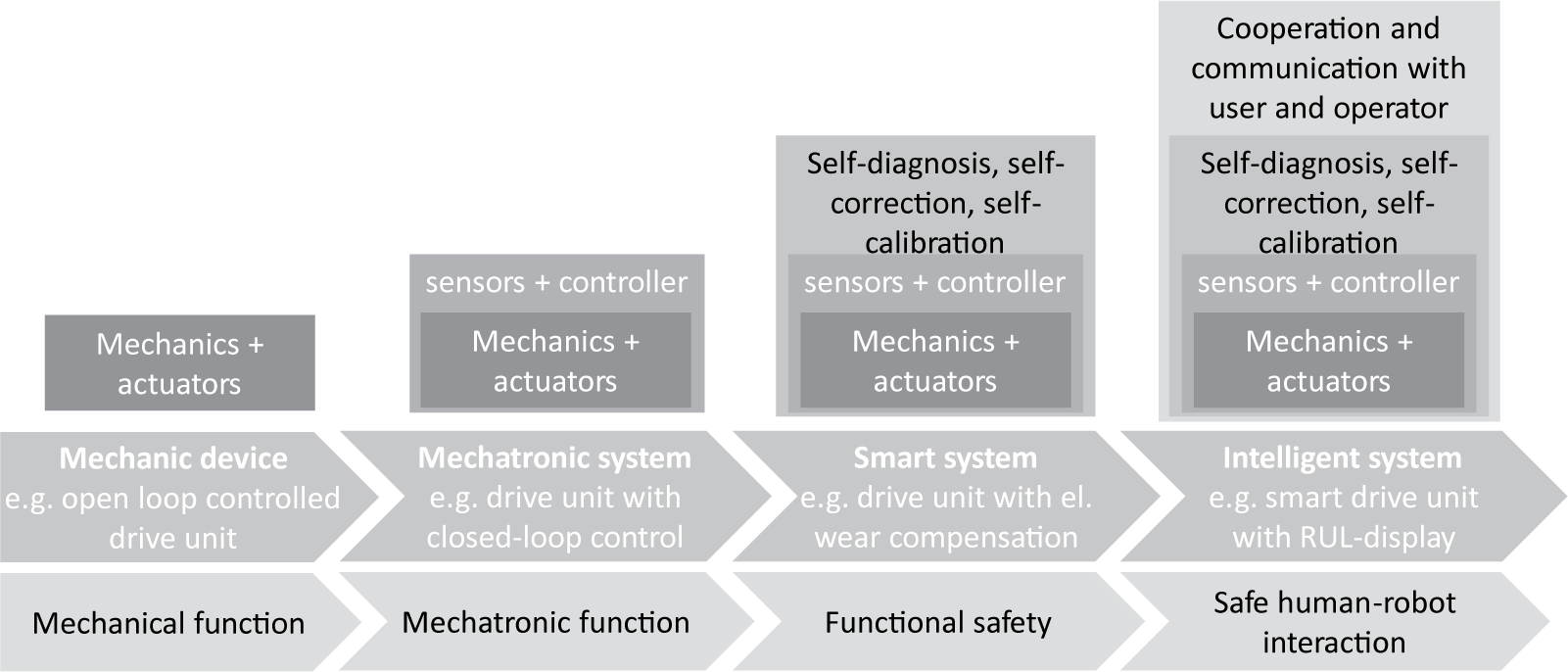
Figure 1. From mechanic devices to intelligent systems (from Vorwerk-Handing et al. Reference Vorwerk-Handing, Gwosch, Schork, Kirchner and Matthiesen2020, based on Anderl et al. Reference Anderl, Eigner, Sendler and Stark2012).
2. Aim of the contribution
Typically, little attention is paid to the reliability of the signal obtained from SME in terms of uncertainty to avoid the gap between established rules on how to handle uncertainty, described, for example, in the guide to the expression of uncertainty in measurement (GUM) (Joint Committee for Guides in Metrology 2008), and the novel concept of SME. Consequently, the target of this contribution is to describe an approach which closes this gap by quantitatively describing and classifying uncertainty in SME and sensing technology in general. This classification can then be used as an indicator of how and where occurring uncertainty could be reduced by means of robust design to improve the reliability, that is, robustness, of the signal obtained. For this purpose, the understanding and classification of uncertainty from the Collaborative Research Centre (CRC) 805 as well as its linkage to robust design strategies and principles are described and subsequently used to develop a quantitative model to determine the impact of uncertainty on a measuring signal. Finally, the proposed approach is applied to a sensing timing belt, as exemplary SME, to reduce and eliminate the impact of occurring uncertainty and thus improve their functionality and applicability.
3. Fundamentals and state of research
At the Technical University of Darmstadt, research on uncertainty has been conducted in the CRC 805 ‘Mastering Uncertainty in Load-Bearing Systems of Mechanical Engineering’ funded by the Deutsche Forschungsgemeinschaft (DFG, German Research Association) (cf. Pelz et al. Reference Pelz, Groche, Pfetsch and Schaeffner2021). Since this contribution is built upon the results of the CRC 805, the state of research mainly focuses on those. Subsequent research, which is also attributable to the CRC 805 and applies to data acquisition problems using sensing technology, SME in particular, is summarised in the following.
3.1. Previous work
Engelhardt et al. (Reference Engelhardt, Birkhofer, Kloberdanz and Mathias2009) proposed an holistic framework, the uncertainty mode and effects analysis (UMEA), for the analysis of uncertainty in load-carrying structures and their evaluation based on the caused effect on the functional performance of a considered system (cf. Engelhardt et al. Reference Engelhardt, Birkhofer, Kloberdanz and Mathias2009; Engelhardt Reference Engelhardt2012). The structure and examples for suitable models and methods supporting each step of the UMEA are shown in Figure 2. The UMEA was utilised by Würtenberger to manage the effects of uncertainty in product models for development purposes but also made the transfer to mathematical product models (cf. Würtenberger et al. Reference Würtenberger, Lotz, Freund and Kirchner2017; Würtenberger Reference Würtenberger2018). Moreover, the UMEA was carried over to the field of sensor uncertainty by Vorwerk-Handing et al. and linked to some examples of SME (cf. Vorwerk-Handing, Welzbacher & Kirchner Reference Vorwerk-Handing, Welzbacher and Kirchner2020; Vorwerk-Handing Reference Vorwerk-Handing2021). Eifler analysed the effect of uncertainty along the product life cycle and evaluated the usability of the UMEA from a different perspective (cf. Eifler Reference Eifler2015). Freund focused on mechanical robust design approaches using the variation management framework (VMF) proposed by Howard et al. (Reference Howard, Ebro, Eifler, Pedersen, Göhler, Christiansen and Rafn2014) to differentiate the effect of robust design measures (cf. Freund et al. Reference Freund, Würtenberger, Lotz, Rommel and Kirchner2017; Freund Reference Freund2018). Lotz finally analysed the effects of uncertainty arising on product families due to similarity (cf. Lotz Reference Lotz2018). For this purpose, Lotz (Reference Lotz2018) applied a nondimensional calculus to understand size dependencies and to identify contradicting growth laws. The effects analysed by Lotz (Reference Lotz2018) need to be considered when assessing functional limits of, for example, sensory rolling bearings, in which the electric capacitance of the lubrication film is used as a sensory effect. When analysing the effects of loaded and unloaded rolling contacts in a rolling bearing, as described by Schirra et al. (Reference Schirra, Martin, Puchtler and Kirchner2021), based on the analysis and modelling of electric damage effects, it turns out that the growth laws describing size dependencies will imply boundary conditions. From this point of view, the use of sensory rolling bearings can be considered as a wildcard when looking at robust design, due to the highly complex, empirical, model necessary to implement the sensory function, cf. Schirra et al. (Reference Schirra, Martin, Puchtler and Kirchner2021).
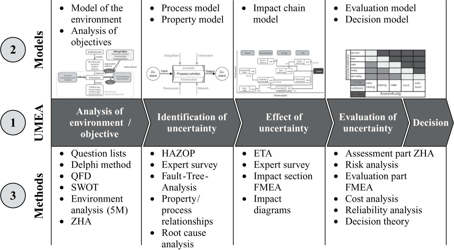
Figure 2. Structure of the uncertainty mode and effects analysis (UMEA) (translated from Engelhardt Reference Engelhardt2012).
3.2. Uncertainty: definition, classification and variation management framework
In the ISO-Guide 73 (2009), uncertainty is defined as ‘state, even partial, of deficiency of information related to understanding or knowledge of an event, its consequence, or likelihood’ (ISO-Guide 73 2009). This definition is used in the following.
There are different approaches in engineering to categorise uncertainty, for example, based on its nature, level or manifestation in the system model (cf. Walker et al. Reference Walker, Harremoes, Rotmans, van der Sluijs and van Asselt2003; Olausson & Berggren Reference Olausson and Berggren2010; Kreye, Goh & Newnes Reference Kreye, Goh and Newnes2011). Uncertainty can be classified as depicted in Figure 3, combining the classification of uncertainty according to its nature – based on the type of relationship between information and uncertainty – and level – based on the amount of available and reliable information. Further details about these two classification approaches are provided by Walker et al. (Reference Walker, Harremoes, Rotmans, van der Sluijs and van Asselt2003) and Olausson & Berggren (Reference Olausson and Berggren2010).
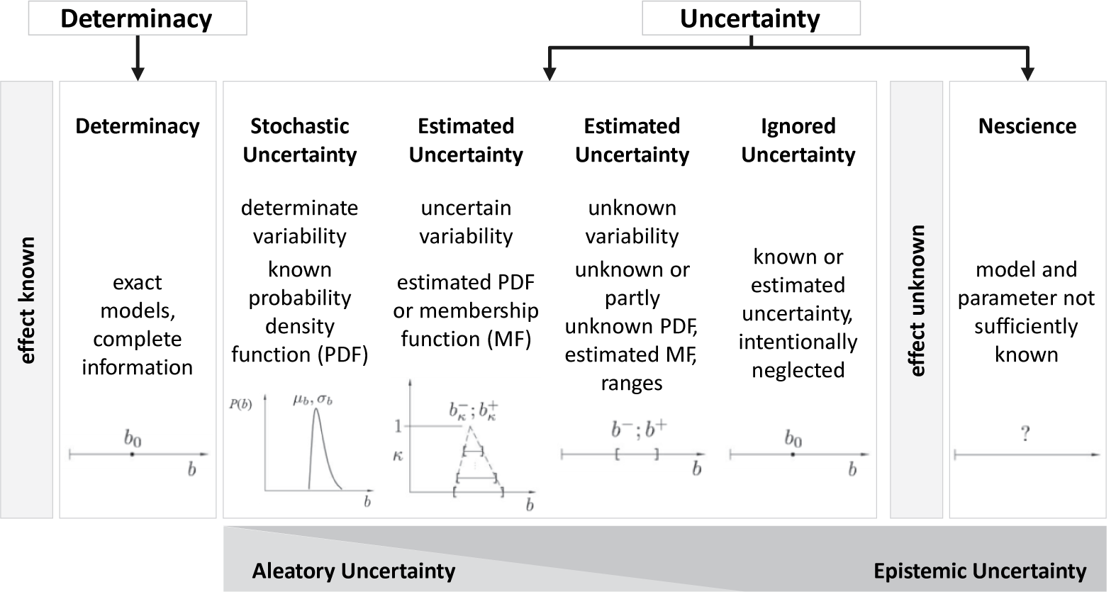
Figure 3. Classification scheme for uncertainty (following Lotz Reference Lotz2018).
In this classification scheme, uncertainty is generally distinguished from determinacy, which describes a condition where exact models and complete information about all relevant parameters exist. It has to be noted that determinacy is an ideal theoretical condition, whereas real technical systems are always subject to uncertainty. Uncertainty itself can range from stochastic uncertainty, where its variation and its probability are known, to nescience, where neither the disturbing influencing parameter nor the disturbance’s cause or a model for describing the interrelations between influencing parameters and the system are sufficiently known. Nescience comprises cases, where uncertainty is suspected but its effects remain unknown. Between these extremes, gradations of uncertainty were defined, based on the amount of available and reliable information. If the probability density function of the output parameter is not known exactly, as for stochastic uncertainty, an estimated probability density function can be applied. The estimated function is categorised under estimated uncertainty and describes the occurrence of a variation of influencing parameters based on known intervals of input–output relationships. In the category of estimated uncertainty, the unknown variability of the output depending on the input is also included. A special case is ignored uncertainty. In this category, the variation is known or estimated but is neglected on purpose, like, for example, in terms of simplifications in the modelling process (cf. Lotz Reference Lotz2018; Pelz et al. Reference Pelz, Groche, Pfetsch and Schaeffner2021).
The impact of uncertainty on a technical system – and consequently sensing technology – as well as its sensitivity to parameter variations becomes notable within the VMF proposed by Howard et al. (Reference Howard, Ebro, Eifler, Pedersen, Göhler, Christiansen and Rafn2014). It visualises how variations, in Figure 4 process properties, propagate via transfer functions through different domains to a measure of interest, in case of Figure 4 the customers’ satisfaction. The final result is influenced by the three linked, sequential steps of production, development and customer perception as depicted. Each transfer function describes the relation of process properties to design parameters during the production, the design parameters towards the system behaviour by the development and finally the system behaviour and the customer’s satisfaction by the customers’ perception (cf. Howard et al. Reference Howard, Ebro, Eifler, Pedersen, Göhler, Christiansen and Rafn2014, Reference Howard, Eifler, Pedersen, Göhler, Boorla and Christiansen2017). How exactly a scattering impacts the measure of interest, in this case, the costumers perception, can be understood as uncertainty.
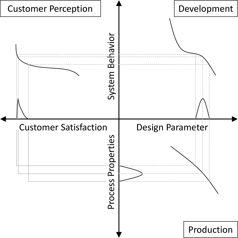
Figure 4. Variation management framework (translated from Freund Reference Freund2018, based on Howard et al. Reference Howard, Eifler, Pedersen, Göhler, Boorla and Christiansen2017).
For the design of and with sensing technology, in particular SME, the consideration of uncertainty is of great importance, since occurring uncertainty can limit their functionality and thus have a significant impact on the benefit of their application. Consequently, uncertainty needs to be systematically identified, mathematically described, to be able to quantify its effects, and considered when designing sensing technology or technical systems with integrated sensing technology, to ensure their functionality. Therefore, for example, the UMEA proposed by Engelhardt et al. (Reference Engelhardt, Birkhofer, Kloberdanz and Mathias2009) is applicable. Applying the VMF in the framework of the UMEA clarifies, at which step uncertainty arises within the development of and with sensing technology and thus how it can be eliminated or at least reduced by applying robust design. During the design of and with sensing technology, uncertainty can occur, for example, in the following forms (cf. Vorwerk-Handing et al. Reference Vorwerk-Handing, Welzbacher and Kirchner2020; Vorwerk-Handing Reference Vorwerk-Handing2021):
(i). manufacturing uncertainty, tolerances and uncertainty due to calibration;
(ii). modelling uncertainty of the relation between the input and output of the sensing technology;
(iii). uncertainty caused by disturbances of/in the usage phase of the system as further described in Taguchi, Chowdhury & Wu (Reference Taguchi, Chowdhury and Wu2004) and Pelz et al. (Reference Pelz, Groche, Pfetsch and Schaeffner2021).
Since SME are based on standardised conventional machine elements that can normally be manufactured within narrow tolerances, in terms of, for example, geometry or material properties, manufacturing uncertainty of SME mainly arises from the additional nonstandardised components required for the realisation of integrated measuring functions. Furthermore, the sensory function of SME, thus the relation between the input – the process or state variable to be measured – and the actually recorded and subsequently interpreted output has to be modelled based on the used physical effects and their corresponding individual laws. For this purpose, physical effect catalogues, for example, the one proposed by Vorwerk-Handing (Reference Vorwerk-Handing2021), can be used. The resulting model finally underlies uncertainty due to, for example, simplifications, made consciously or unconsciously, unknown disturbances or the temporal change of included design parameters, for example, due to corrosion or wear. These aspects are related to the SME itself and can in general be determined for each SME. In addition, when designing with SME, uncertainty arises due to the integration of the SME into a technical system, which needs to be considered, too. The uncertainty results, for example, from a change in the environmental conditions or a different assembly situation compared with standard testing conditions. These system aspects have to be investigated for each technical system using SME and taken into account (cf. Kreye et al. Reference Kreye, Goh and Newnes2011; Vorwerk-Handing et al. Reference Vorwerk-Handing, Gwosch, Schork, Kirchner and Matthiesen2020; Hausmann et al. Reference Hausmann, Koch and Kirchner2021).
3.3. Robust design
Uncertainty in different areas of the mechanical engineering domain can be addressed by applying robust design during the product development process to achieve insensitivity, that is, robustness, of a technical system against this uncertainty. A technical system is defined as ‘robust’ when it is able to ‘[…] fulfill its predefined functions [not only] at the design point, but also in the surrounding neighborhood […]’ (Pelz et al. Reference Pelz, Groche, Pfetsch and Schaeffner2021). This definition is similar to the understanding of robustness by Taguchi et al. (Reference Taguchi, Chowdhury and Wu2004), which is often used in this context, who defines a system or process as robust ‘[…] when it has limited or reduced functional variation, even in the presence of noise’.
To achieve robustness of a technical system, Mathias et al. (Reference Mathias, Kloberdanz, Engelhardt and Birkhofer2010) defined three strategies, so-called robust design strategies, for handling disturbances causing uncertainty. These can already be applied in the development phase of the system. They differ, as shown in Figure 5, with regard to their individual starting point in the influencing chain of the disturbances:
(i). Elimination of the disturbance: prevent the disturbance from coming up at all.
(ii). Suppression of the influence of the disturbance: prevent the caused influence of the disturbance from acting on the (sub)system.
(iii). Reduction of the impact of the disturbance: prevent the impact of the disturbance from influencing the behaviour of the system considered and consequently causing problematic effects.
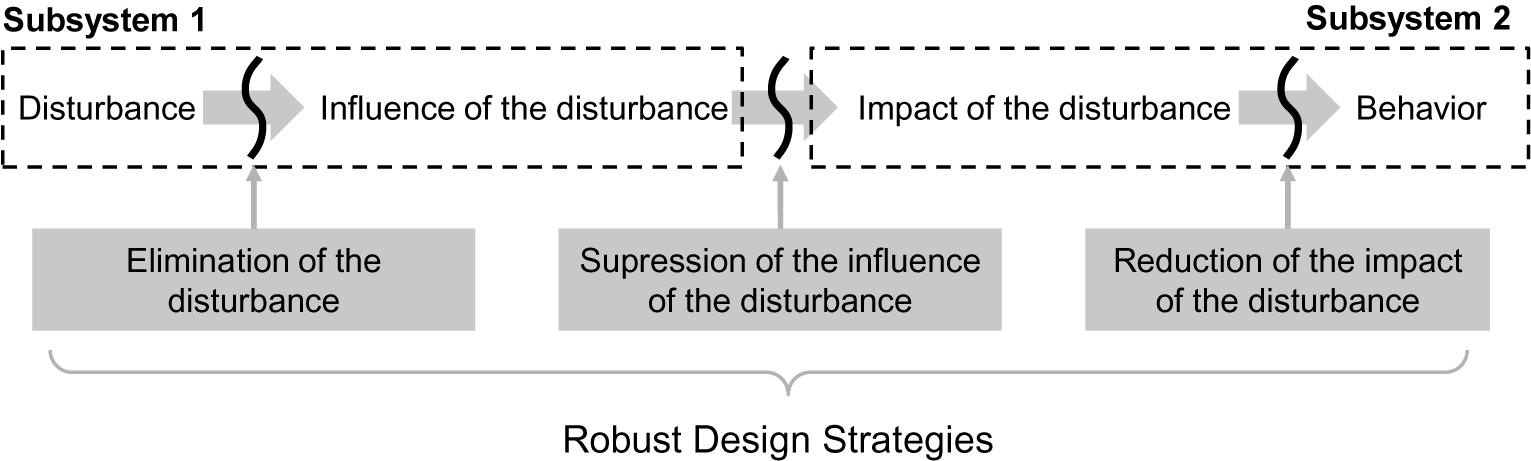
Figure 5. Robust design strategies (based on Mathias et al. Reference Mathias, Kloberdanz, Engelhardt and Birkhofer2010).
To implement these strategies in the development phase of a technical system, Ebro and Howard proposed different robust design principles (cf. Ebro & Howard Reference Ebro and Howard2016; Howard et al. Reference Howard, Eifler, Pedersen, Göhler, Boorla and Christiansen2017). These principles are categorised according to their influence, to be applicable for handling variations of the design parameters, influencing the sensitivity of the system towards the variation of design parameters and for handling the variation of the system’s behaviour. All principles contribute to the reduction of the variation of behaviour as depicted in Figure 6.

Figure 6. Robust design in the development phase using principles for influencing the transfer function between design parameters and the product behaviour following Ebro (translated from Freund Reference Freund2018, based on Ebro & Howard Reference Ebro and Howard2016; Howard et al. Reference Howard, Eifler, Pedersen, Göhler, Boorla and Christiansen2017).
4. A formal approach to classify uncertainty effects in sensing technology
In the following, an abstracted signal chain of a measurement setup using a SME, shown in Figure 7, is considered. This representation is not limited to SME, but can also be used for sensing technology in general. In Figure 7, each box symbolises a transformation of a quantity, which can in principle be influenced by uncertainty caused by a disruption. The signal chain starts at the measuring object, where the measurand  $ \Phi $ occurs as a function of different state variables like, for example, temperature $ \vartheta $, voltage $ U $, current $ I $ and mechanical properties like force $ F $, torque $ T $ and acceleration $ a $. The measurand $ \Phi \hskip1.5pt \in \hskip1.5pt {\left\{F,T,a,\vartheta, U,I,\dots \right\}}^T $ is measured by the SME or sensing technology, respectively, and transformed into a signal. The signal emitted by the SME $ S $ is then transferred to the process control unit, where the signal $ {S}^{\ast } $ is received. The whole signal chain is subject to uncertainty as indicated by the flash icon in Figure 7, which comprises the uncertainty arising from each transformation within the signal chain. For example, uncertainty can be caused by the measuring object due to simplifications in the relation between the actual quantity of interest and the measurand. It can also arise in the energy transfer, for example, due to parasitic currents in case of a structure-integrated transfer path via mechanical elements.

Figure 7. Schematic integration of sensing machine elements into mechatronic systems.
For the subsequent mathematical description of uncertainty, we consider an uncertainty  $ \Delta x $ of a quantity $ x $ associated to the SME, or sensing technology in general, respectively, that influences the relation $ f $ between the measurand $ \Phi $ and the signal $ S $, causing a deviation of the emitted signal $ \Delta S $ and consequently a deviation $ \Delta {S}^{\ast } $ of the signal received by the process control unit. It is assumed that the function $ f $ is sufficiently accurate for modelling the dependency between the governing quantities $ x $ and the sensor signal $ S $. Uncertainties such as geometric tolerances disabling the assembly of, for example, a bolt–bore pair need to be given special attention since they have an impact on the overall system performance. In that sense, the discussion needs to be limited to disturbances which do not cause discontinuities in the primary function of the product or system. For the following explanations, it is assumed that the uncertainty associated to the measuring object as well as the energy transfer has little influence on the signal received by the process control unit compared with the uncertainty associated with the SME itself and the signal transfer. As the sensor is brought closer to the measurand, influences on its transmission through the system are diminished and therefore the uncertainty of the recorded signal is reduced. In turn, the uncertainty is shifted towards the signal transfer. What sounds like a mere benefit at first, contains drawbacks as the transfer out of a technical system is most certainly problematic. For example, in rotating machines where a wired signal transfer is impossible, wireless transmission is inevitable but might be compromised by surrounding electric or magnetic fields. The concept of energy transfer is regarded to be independent from the SME as long as the measuring is passive.
4.1. Quantitative description of uncertainty
As mentioned in Section 3.2, the classification scheme for uncertainty distinguishes between the categories ‘determinacy’, ‘stochastic uncertainty’, ‘estimated uncertainty’, ‘ignored uncertainty’ and ‘nescience’, cf. Figure 3, depending on how much information about uncertainty and the caused effect is known and thus how precise it can be described in terms of modelling. This classification is not limited to mechanical systems, but is also applicable to signal transfer analysis. The mathematical expressions introduced in the following are summarised in Figure 8. They allow a formal description of the uncertainty-effect relation and to identify suitable calculation methods, for instance Gaussian error propagation, to quantify the final effect caused by uncertainty.

Figure 8. Classification of uncertainty (utilising basic definitions from Knetsch Reference Knetsch2004; Engelhardt Reference Engelhardt2012).
The ideal case would be determinacy, which means complete knowledge about the system and influences on the systems would exist. Consequently, the effects of uncertainty on the signal emitted by the SME and its probability could be explicitly determined. The caused effects on the system could be described mathematically without a lack of model parameters. Depending on the type of disturbances identified, different possibilities would exist to describe the effect of the disturbance on the system. If the disturbance is continuous, it can be mathematically described following Eq. (1), whereby the derivation of the function indicates the sensitivity of the system to this disturbance.
 $$ S\hskip1.5pt =\hskip1.5pt f(x)\iff \Delta S\hskip1.5pt =\hskip1.5pt {\left.\frac{\mathrm{d}f}{\mathrm{d}x}\right|}_x\cdot \Delta x. $$
The evaluation of the derivative at the nominal design point  $ x $ in Eq. (1) assumes, as mentioned earlier, that the model $ f $ is sufficiently smooth and continuous. Provided that the primary functions remain unaffected by the influence of the disturbance $ \Delta x $. If the sensory function shows any kind of discontinuity, the determinacy condition for Eq. (1) is violated. If stochastic uncertainty occurs, it has a known effect on the system but cannot be fully quantified. However, the character and extent of the impact are known to have a certain probability density function and can be considered during the system development. This leads to a direct dependency of the signal variation $ \Delta S $ on the uncertainty $ \Delta x $, which is described through Eq. (2). Therefore, the continuity of the uncertainty is assumed, too.
 $$ S\hskip1.5pt =\hskip1.5pt c+k\cdot {x}^m\iff \Delta S\hskip1.5pt =\hskip1.5pt k\cdot m\cdot {x}^{m-1}\cdot \Delta x. $$
Estimated uncertainty is present if partial information about the value of influencing parameters, their impact and/or the probability of occurrence are not known. It is distinguished between an uncertain variability and an unknown variability. For uncertain variability, the probability density functions or assignment functions are estimated and one of the model parameters  $ k $ and $ m $ remains undetermined, cf. Eq. (3). This leads to a loss of prediction accuracy. The effect of an uncertainty $ \Delta x $ can only be expressed in a vicinity of the current design state.
 $$ S\hskip1.5pt \propto \hskip1.5pt {x}^m\iff \Delta S\hskip1.5pt \propto \hskip1.5pt {x}^{m-1}\cdot \Delta x. $$
The combination of Eqs. (1)–(3) leads to the conclusion that effects of uncertainty can be described almost completely for the first two cases, whereas dependencies can only be stated for the third case. For unknown variability, the probability density functions or assignment functions are known or partly unknown and a tendency statement can be given but no precise quantity can be calculated. The leading power  $ m $ in Eq. (3) is often known but the coefficient is not. Consequently, only rough guesses can be stated for unknown variability, which are rather tendency estimates, as described with Eq. (4).
 $$ \Delta S\propto \pm \Delta x. $$
Disregarded uncertainty is characterised by the fact that the effects of disturbances are deliberately neglected, mostly based on some intuitive estimates to limit the complexity of the description. The effects of uncertainty itself can be of any type described, they might be understood but excluded.
Unknown uncertainty, analogue to nescience in the classification scheme from Figure 3, is characterised by the absence of applicable engineering intuition. Therefore, the system behaviour is not predictable by the engineer. Estimates of the occurring uncertainty cannot be made explicit due to, for example, contradicting dependencies. None of the dependencies described in Eqs. (1) through (4) can be applied to estimate the effects of uncertainty.
4.2. Consideration of uncertainty in the transfer path
For the consideration of uncertainty, the signal chain shown in Figure 7 can be used as a guideline to determine the sensitivity of a signal with respect to occurring uncertainty, which affects the signal on its way from the measurand  $ \Phi $ to the process control unit, where a signal $ {S}^{\ast } $ is received.
Under the assumption that determinacy is present and the relation between the measured  $ \Phi $ and the emitted signal $ S $ is completely known, the sensitivity of the sensing technology can be calculated as described in Eq. (5) with regard to variations in both the measurand $ \Phi $ and the uncertainty affected quantity $ x $.
 $$ S\hskip1.5pt =\hskip1.5pt f\left(\Phi, x\right)\iff \Delta S\hskip1.5pt =\hskip1.5pt {\left.\frac{\partial f}{\mathrm{\partial \Phi }}\right|}_{\Phi, x}\cdot \Delta \Phi +{\left.\frac{\partial f}{\partial x}\right|}_{\Phi, x}\cdot \Delta x. $$
In case the relation  $ f $ between the measurand $ \Phi $ and the emitted signal $ S $ cannot be completely described including all relevant and consequently required parameters, the derivatives in (1) cannot be determined, leaving in best case a tendency statement in form of Eq. (2). Hence, if this relation cannot be fully described, there is at least estimated uncertainty present, which allows only trend predictions.
Since uncertainty not only arises within the transformation of the measurand  $ \Phi $ into the emitted signal $ S $, but also the signal transfer turning the emitted signal $ S $ into $ {S}^{\ast } $, both transformations must be considered. The argumentation applied in terms of sensing technology can also be applied to the signal transfer. Hence, considering an additional uncertainty $ \Delta \tilde{x} $ arising within the transformation of the emitted signal $ S $ into $ {S}^{\ast } $, described by the function $ g $, the sensitivity of the signal transfer can be calculated as shown in Eq. (6).
 $$ {S}^{\ast }=g\left(S,\tilde{x}\right)\iff \Delta {S}^{\ast }={\left.\frac{\partial g}{\partial S}\right|}_{S,\tilde{x}}\cdot \Delta S+{\left.\frac{\partial g}{\partial \tilde{x}}\right|}_{S,\tilde{x}}\cdot \Delta \tilde{x}. $$
Consequently, the accumulated effect  $ \Delta {S}^{\ast } $ of the uncertainty portions $ \Delta x $ and $ \Delta \tilde{x} $ on the signal received at the process control unit can be described following (7).
 $$ \Delta {S}^{\ast }={\left.\frac{\partial g}{\partial S}\right|}_{S,\tilde{x}}\cdot \left\{{\left.\frac{\partial f}{\mathrm{\partial \Phi }}\right|}_{\Phi, x}\cdot \Delta \Phi +{\left.\frac{\partial f}{\partial x}\right|}_{\Phi, x}\cdot \Delta x\right\}+{\left.\frac{\partial g}{\partial \tilde{x}}\right|}_{S,\tilde{x}}\cdot \Delta \tilde{x}. $$
The challenge is, however, to differentiate a change in the signal received  $ \Delta {S}^{\ast } $ by its reason, being caused by either occurring uncertainty or in fact by a change of the measurand $ \Delta \Phi $.
To interpret the reason for a change of the signal received by the process control unit, it is indispensable to understand all differential expressions in Eq. (7). Therefore, all dependencies must be fully determined, which would allow the application of Eq. (1). Oftentimes, engineers try to bypass this problem of limited knowledge by applying additional sensors, for example, a thermocouple to record a drift in temperature. Using this thermocouple, a change in the signal received by the process control unit, which is caused by a thermally induced uncertainty, can be clearly related to the drift in temperature once the temperature sensitivity is known. But, as long as the sensitivity is unknown, not even in the form of Eqs. (2) or (3), one can only guess – but not quantitatively describe – the reason for the change of the received signal  $ \Delta {S}^{\ast } $.
This approach always targets at moving individual entries in Eq. (7) up in the hierarchy of managed uncertainty starting from Eqs. (4) to (1). In doing so, estimated uncertainty is gradually reduced to stochastic uncertainty resulting theoretically in determinacy, which would allow the correct interpretation of the different root causes of a signal change  $ \Delta {S}^{\ast } $ when uncertainty $ \Delta x $ and $ \Delta \tilde{x} $ are either excluded or measured by individual sensors denoting their change.
The mathematical description of a system or part of it, respectively, provides an opportunity to objectively determine the uncertainty category of the corresponding model. The classification of uncertainty then leads to useful measures how and where to eliminate or gradually reduce disruptions causing uncertainty – in terms of robust design. Furthermore, an already existing system model allows a step by step concretisation, in which the reduction of uncertainty can be tracked by comparing the mathematical description before and after the concretisation and subsequently re-categorising according to the descriptions in Figure 8. The aim of the concretisation is to identify, which information is still required about the system, its behaviour or its interrelations so that the model follows a stochastic uncertainty behaviour in the end. This makes the data acquisition with sensing technology, in particular SME, a robust, and hence an applicable and useful, tool. In the following section, an example is discussed to outline the resulting robust design process.
5. Application example, the sensing timing belt
The above-described approach for the quantitative description of uncertainty and the resulting robust design process is now applied to the sensing timing belt by Großkurth & Martin (Reference Großkurth and Martin2019) as an exemplary SME. The quantity of interest for maintaining belt drives is the timing belt’s wear. The sensing timing belt enables an in situ measurement of the span-specific belt force during operation, which corresponds directly to the wear. Thus, the sensing technology extends the mechanical primary function of a conventional timing belt (cf. Großkurth & Martin Reference Großkurth and Martin2019).
The belt force is divided into its pretension and the drive torque, which leads, for a two pulley drive, to one span with a higher belt force (tight span) and one span with a lower belt force (slack span). The pretension is key for an effective and efficient torque transmission between two or more toothed pulleys. Wear, due to tear and fretting of the tension members, reduces the timing belt’s stiffness. Moreover, the stiffness change can serve as an indicator for the current wear. A CAD-model showing the concept and a prototype of the sensing timing belt by Großkurth & Martin (Reference Großkurth and Martin2019) are shown in Figure 9.

Figure 9. CAD-model and prototypically realised concept of the sensing timing belt (cf. Großkurth & Martin Reference Großkurth and Martin2019).
During operation, a timing belt is subject to a broadband vibration excitation, mainly caused by the polygon effect. For further information about the polygon effect, please refer to, for example, Nagel (Reference Nagel2008) or Perneder (Reference Perneder2009). The sensor module and a lithium ion accumulator, as energy supply, are adhesively embedded into two neighbouring pockets which are milled out of the timing belt teeth. The span-specific belt force of the sensing timing belt is measured indirectly via the eigenfrequencies of the vibrating belt using MEMS-acceleration sensors (cf. Großkurth & Martin Reference Großkurth and Martin2019). The timing belt conducts as a string and the span-specific belt force is calculated using the string equation, cf. Figure 10. The measuring function of the sensing timing belt can be described on a basic level using physical relationships, generally referred to as effect chain, which is shown for the sensing timing belt in Figure 10. The transfer of Figure 7 for the example is shown in Figure 11 for better understanding.

Figure 10. Effect chain of the measuring function of the sensing timing belt.
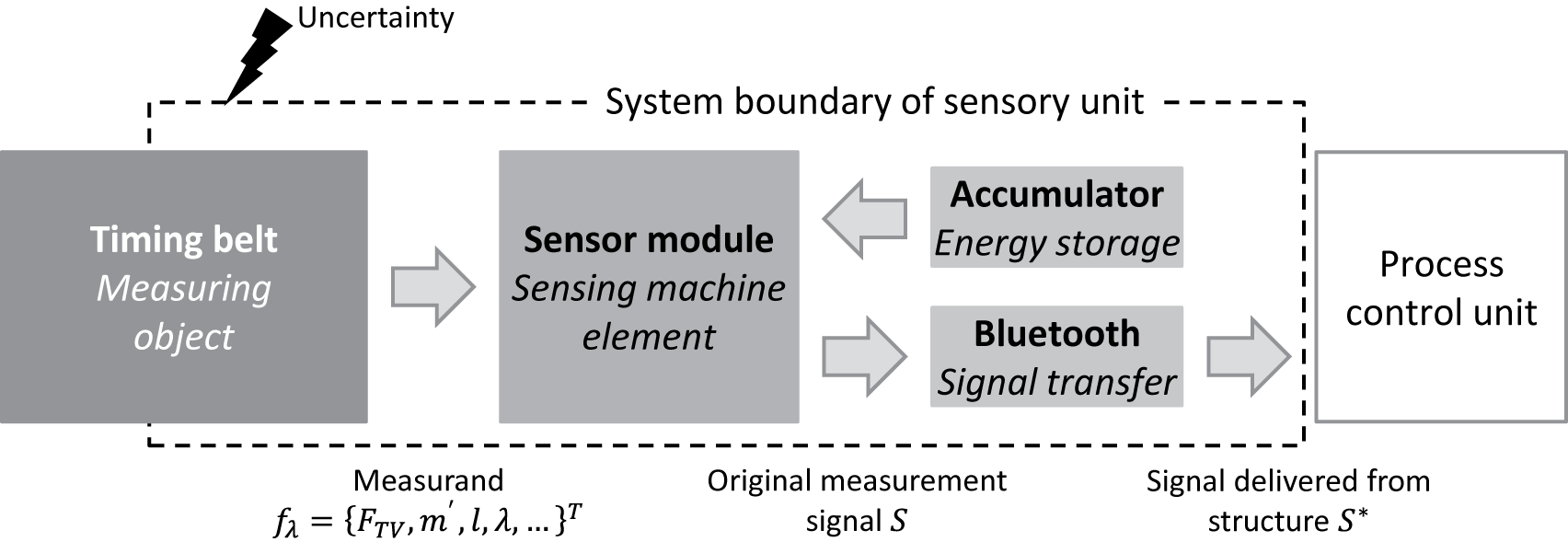
Figure 11. Schematic description of the sensing timing belt and its components (based on Großkurth & Martin Reference Großkurth and Martin2019).
Based on the effect chain of the measuring function of the sensing timing belt, the therein-included quantities as well as first experimental studies using prototypes, Großkurth & Martin (Reference Großkurth and Martin2019) identified torsional vibrations and heat transmission as main disturbances impacting the sensory function. As long as these are neither determined nor prevented, this results in uncertainty. Both disturbances originate from the environment of the timing belt and are therefore highly application-dependent. Consequently, these sources cannot be described or quantified in a general way, which is why unknown uncertainty is present. In addition to that, due to their occurrence in the environment, both disturbances are typically located outside the circle of control when designing SME. Hence, it is impossible to directly eliminate this uncertainty; it is only possible to design the sensing timing belt in a way that its sensory function is insensitive to the causing disturbances and therefore robust. This can be achieved in two different ways. On the one hand, additional sensory functions could determine the disturbances, which allow their consideration during the signal evaluation; on the other hand, the technical system might be adopted towards a less sensitive design regarding the disturbances. Both approaches are outlined in the following section, starting with the option of additional sensing technology.
Two measures were implemented in a first design iteration by Großkurth & Martin (Reference Großkurth and Martin2019) to achieve the necessary robustness of the sensing timing belt against uncertainty caused by torsional vibrations and heat transmission. On the one hand, the sensor module of the initial concept was extended by a second MEMS-acceleration sensor and the initial sensor was rearranged. Both sensors are mounted on opposite sides of the PCB perpendicular to the direction of travel of the timing belt with maximum distance from the middle of the timing belt. This makes it possible to clearly differentiate between longitudinal vibrations of the timing belt, which enable the measurement of the timing belt’s eigenfrequencies, and torsional vibrations, caused, for example, by the drive unit, which superpose the longitudinal vibrations. If the output signal of both acceleration sensors is in phase, the measured vibration is a longitudinal vibration, for example, an eigenfrequency of the timing belt. In contrast, if the signals from the sensors are 180° phase shifted to each other, the measured vibration is a torsional vibration and thus needs to be filtered out in the subsequent signal evaluation and interpretation to ensure the correctness of the measurement. On the other hand, a temperature sensor was added to the sensor module of the sensing timing belt. Based on the information provided by this sensor, the thermally induced change in span-specific belt force can be detected and subsequently be compensated during signal evaluation and interpretation.
But not only the robustness of the sensing technology itself is of great importance to ensure the correct measurement outcome. In addition, when designing a technical system with SME also the behaviour of the system itself must be considered. In case of the sensing timing belt, the behaviour of the timing belt drive, in which the timing belt will be used, must also be taken into account to reduce uncertainty in terms of the subsequent interpretation of the signal received by the process control unit. This is due to the fact that different types of timing belt drives commonly used in practice, differ in terms of their behaviour.
For the following explanations, two different types of timing belt drives, shown in Figure 12, are considered. Timing belt drive (a) from Figure 12 consists of two stationary toothed pulleys whereas timing belt drive (b) consists of one stationary and one movable toothed pulley, which is fixed in a sled with an attached weight. If an elongation of the timing belt occurs, for example, due to thermal disturbances, belt drive (b) is able to maintain the belt pretension whereas in belt drive (a), the pretension cannot be maintained. Thus, the measured eigenfrequencies of the sensing timing belt in belt drive (b) change according to Eq. (8), similar to (5), based on the law of the physical effect ‘String’, shown in Figure 10, and the Gaussian error propagation.
 $$ \frac{\partial {f}_{\lambda_{\mathrm{b}}}}{\partial T}\hskip1.5pt =\hskip1.5pt \sum \limits_j\left|\frac{\partial {f}_{\lambda }}{\partial {x}_j}\right|\cdot \frac{\partial {x}_j}{\partial T}\hskip1.5pt =\hskip1.5pt \left|\frac{\partial {f}_{\lambda }}{\partial l}\right|\cdot \frac{\partial l}{\partial T}. $$
Figure 12. Timing belt drive (a) – left and timing belt drive (b) – right (cf. Schlecht Reference Schlecht2007).
In contrast, the eigenfrequencies of the sensing timing belt in belt drive (a) change according to Eq. (9), also based on the physical effect ‘String’ and Gaussian error propagation.
 $$ \frac{\partial {f}_{\lambda_{\mathrm{a}}}}{\partial T}\hskip1.5pt =\hskip1.5pt \sum \limits_j\left|\frac{\partial {f}_{\lambda }}{\partial {x}_j}\right|\cdot \frac{\partial {x}_j}{\partial T}\hskip1.5pt =\hskip1.5pt \left|\frac{\partial {f}_{\lambda }}{\partial l}\right|\cdot \frac{\partial l}{\partial T}+\left|\frac{\partial {f}_{\lambda }}{\partial {F}_{TV}}\right|\cdot \frac{\partial {F}_{TV}}{\partial T}. $$
The additional term in Eq. (9), representing the temperature-induced change in pretension of the timing belt, qualitatively implies that the mounting of the sensing timing belt is less robust towards the disturbance for configuration (a) than it is for (b). Consequently, if the behaviour of the technical system itself is not taken into account while interpreting the received signal of the SME, the change in the signal due to a temperature disturbance would be interpreted as significant change of the measurand wear. In case of the presented example, the monitored part of the system, the timing belt itself, would mistakenly be maintained.
6. Conclusion and outlook
Finally, it is shown that the design of and with sensing technology is challenging and still an open field of research. The robust design framework showed that the application of, in the example case SME, not only requires a deeper understanding of the sensing technology itself, in particular, but also of the technical periphery it will be embedded in. It was demonstrated, that changes in the technical system, which are not incorporated in the analysis of the sensor signal, or eliminated from the beginning, corrupt the information provided by the sensing technology. Consequently, the signal of the SME is misinterpreted and thus the added benefit of being close to the or inside the process vanishes. Robust design strategies during the design process of the sensing technology itself as well as the application of those strategies on the mechanical system in conjunction with the sensing technology are necessary for a successful product development.
The further research needs to focus on the development of robust SME, which implies robust design of the element itself but also considering strategies for their integration into a specific technical system. Both topics are under investigation in a research project funded by the DFG (German Research Association) about the derivation of analysis- and synthesis-methods and therefore suitable models to manage uncertainty in the development of technical systems with SME (Project number: 426030644).
Acknowledgment
This work was funded by the Deutsche Forschungsgemeinschaft (DFG, German Research Foundation) – project numbers: 426030644 and 57157498 – SFB 805.
Competing interest
The authors declare none.


 Open access