


Impact Statement
Data mining and knowledge discovery (DMKD) can be a powerful tool in the analysis of chemical plant data. However, method selection and implementation can be a difficult task. In this contribution, all stages of the DMKD process are considered in detail, examining the fundamentals of various methods as well as practical insights on how to select and tune these methods. Both simulated and real plant data are analyzed to showcase the properties of data cleaning, sampling, scaling, dimensionality reduction, clustering, and cluster analysis, and their applicability in real-life scenarios. Also, a friendly graphic user interface to implement DMKD is presented.
1. Introduction
The increasing complexity of chemical processes along with the requirements for safety, efficiency, and environmental responsibility makes it essential to have agile and fast methods to visualize and interpret plant data. Activities such as product scheduling, fault detection, root cause analysis, and maintenance rely on an accurate representation of the often large and multidimensional datasets generated by plant instrumentation. In addition to the individual instruments and their historic behavior, the interactions between different components of the process can provide vital information about the dynamic behavior of the plant. However, the interpretation of the complete dataset in order to capture the overall state of a given process in a concise way, so that an operator can readily understand it, is not a trivial task. This is especially complex due to the size of the datasets being generated in by the process and the velocity at which more data is added (Ge et al., Reference Ge, Song, Ding and Huang2017). In this context, computational developments in data science and artificial intelligence (AI) have gained great interest in recent years as means to overcome these challenges.
A computational advancement of special interest for chemical process industrial application is data mining and knowledge discovery (DMKD). A typical flowchart for the implementation of DMKD is shown in Figure 1. The goal of DMKD is to train a learning agent (i.e., a model) to find patterns previously unknown in a given data set. The learning agent can recognize such patterns in the data and provide an interpretable representation by performing two main tasks: dimensionality reduction (DR) and clustering. In the former, the high-dimensional space defined by the different variables involved in the system is reduced to a low-dimensional representation (typically 2-D or 3-D) (Tan et al., Reference Tan, Steinbach and Kumar2016). In the latter, a measure of similarity is used to find relationships among the low-dimensional embedded datapoints. The result is a visually accessible and quick to understand description of the system in which relevant patterns have emerged (Joswiak et al., Reference Joswiak, Peng, Castillo and Chiang2019). A human agent (i.e., a plant operator) can then interpret those patterns to assign them physical meaning according to the nature of the domain and previous knowledge of the system. In this sense, DMKD helps process the data in such a way that a human agent can understand it and make decisions based on this understanding. Since the human agent relies on the simple low-dimensional representation of the complex high-dimensional original data, the capabilities and limitations of the methods being used must be well understood to ensure the correspondence between the data representation and the actual physical phenomena. Furthermore, although DR and clustering are the main tasks to be performed in DMKD, the previous steps shown in Figure 1, namely data cleaning, sampling, and normalization, play a major role in both the quality and the interpretation of the end result, and therefore should be considered an integral part of the analysis.
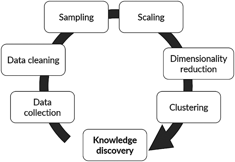
Figure 1. Typical flow of a data mining and knowledge discovery methodology.
DMKD methods have been deployed in the context of chemical processing and manufacturing for a variety of applications. For industrial applications, machine learning (ML) methods are mainly used for information extraction, data visualization, density estimation, outlier detection, and other tasks that are instrumental for process monitoring and visualization (MacGregor and Cinar, Reference MacGregor and Cinar2012; Zhu et al., Reference Zhu, Sun and Romagnoli2018; Joswiak et al., Reference Joswiak, Peng, Castillo and Chiang2019), root cause analysis of faults (Yu and Qin, Reference Yu and Qin2008; Qin, Reference Qin2012; Han et al., Reference Han, Tian, Romagnoli and Li2018), maintenance scheduling (Wocker et al., Reference Wocker, Betza, Feuersänger, Lindworsky and Deuse2020), decision support, life cycle management, product quality assurance, and defect prognosis (Sharp et al., Reference Sharp, Ak and Hedberg2018; Tao et al., Reference Tao, Qi, Liu and Kusiak2018; Zhao et al., Reference Zhao, Dinar and Melkote2020). All these applications are closely related to the concept of smart manufacturing (Christofides et al., Reference Christofides, Davis, El-Farra and Clark2007) and the effective use of digital technologies for the improvement of chemical plants. Conventionally applied DMKD methods in the process industry include principal component analysis and its variations, K-Means clustering, kernel density estimation, self-organizing maps, Gaussian mixture models, manifold learning, and support vector data description (Qin, Reference Qin2012; Ge et al., Reference Ge, Song, Ding and Huang2017). In addition to these methods, a variety of new DMKD implementations are being continuously developed and as the number of options available increases, so does the need for an understanding of their applicability in industrial settings.
While an increasing amount of industries start to incorporate both classical and new DMKD methodologies, there are still some challenges limiting more widespread usage of these new methods (Chiang et al., Reference Chiang, Lu and Castillo2017). One challenge is that of navigating the variety of methods available and selecting the 1 best suited for a given application, while considering the benefits, risks, and ease of implementation. Furthermore, the tuning of the DR and clustering algorithms’ hyperparameters might have a great impact on performance and reproducibility (Wuest et al., Reference Wuest, Weimer, Irgens and Thoben2016). Also, and no less important, is the challenge of data preprocessing and data preparation which has shown to be highly time consuming in real-life applications (Chiang et al., Reference Chiang, Lu and Castillo2017; Dogan and Birant, Reference Dogan and Birant2021). The path to overcome these challenges would include the development of algorithms with few hyperparameters oriented to mitigate these problems and able to deal with imperfect datasets. Furthermore, and perhaps more immediate, a sound working knowledge of the foundations of these methods so that an informed decision can be made for their selection, and their implementation can be streamlined. This work focuses on the latter, aiming to provide some practical insights for the deployment of DMKD methods in the process industries.
In this contribution, DMKD was implemented using a variety of data preprocessing, DR, clustering, cluster analysis, and visualization methods to examine the behavior of 2 different chemical plants: a simulated natural gas liquid plant and a real pyrolysis reactor. By producing simulated data that included both global (e.g., general plant behavior) and local (e.g., controller dynamics) changes, the ability of different DMKD ensembles to effectively detect useful patterns in these 2 scenarios is demonstrated. The effect of data preprocessing methods is also reported. The use of simulated data allows for verification of findings (since the actual causes of the systems’ behavior are known) while the use of real data shows the applicability of these methods in real-life scenarios. Furthermore, the use of self-organized maps as a visualization method for both the verification of the clustering results and the tracking of plant drift through an operation cycle for unsteady-state processes is demonstrated. Additionally, a user-friendly graphical user interface (GUI) called FastMan (Fast Manual data classification) was developed that conveniently allows for the analysis of datasets not limited to the methods described here, with no programming knowledge required, is presented. This framework could help extend the use of DMKD methods in real plant settings and provide a starting point for future developments in automated ML applications in chemical processes.
The rest of this article is structured as follows: first, an overview of the relevant theoretical aspects is presented. Second, the computational tools used in this investigation are described, including the GUI developed. Third, two case studies are used to illustrate the DMKD workflow and the insights that can be obtained from these analyses. For each case study, a description of the process and the way the methods were implemented is presented. Finally, a number of conclusions derived from the 2 case studies are proposed.
2. Theoretical Background
2.1. Data preprocessing
Data preprocessing is essential to improve data quality, which in turn might have a dramatic effect on the subsequent steps in the DMKD implementation. For instance, outliers and gross errors represent extreme values far outside the statistical distribution of practical measurements and, if not purged from the physically relevant data, could affect the estimates, confidence regions, and other tests performed on the data. Because of the effect outliers can have on the integrity of a dataset, their detection and removal are crucial before further analysis (Pearson, Reference Pearson2002; Liu et al., Reference Liu, Shah and Jiang2004; Corona et al., Reference Corona, Mulas, Baratti and Romagnoli2012; Wang et al., Reference Wang, Mao and Huang2018). Also, missing data may arise in process databases from instrument or software errors, and must be addressed (e.g., deletion of the sample, missing value estimation) to ensure the integrity of the data analyses (Imtiaz and Shah, Reference Imtiaz and Shah2008; Xu et al., Reference Xu, Lu, Baldea, Edgar, Wojsznis, Blevins and Nixon2015; Ge et al., Reference Ge, Song, Ding and Huang2017). Another issue to consider is the scale of different variables. In order to prevent the model from relying more heavily on a single variable just because of its relative magnitude with respect to other variables, a proper scaling must be performed (Ge et al., Reference Ge, Song, Ding and Huang2017). However, this data preprocessing step needs to be considered carefully, since some models or learning tasks may have requirements on different scales for different variables (García et al., Reference García, Luengo and Herrera2015).
2.1.1. Data cleaning and outlier removal
An outlier is an anomaly that does not follow the statistical distribution of the bulk of the data and can be heavily influential on the data analysis. On smaller data sets, outliers can be removed simply through visual inspection. For larger data sets, however, this approach would be extremely inefficient so an algorithmic method should be used.
Two methods used for outlier detection are z-score and k-nearest neighbor (kNN). The z-score is a simple method for outlier detection on each individual variable of the dataset. The z-score indicates how far the value of the data point or sample is from its mean for a specific variable. For example, a z-score of 1 means the sample point is 1 standard deviation away from its mean. Typically, z-score values greater than or less than +3 or −3, respectively, are considered outliers. The z-score is expressed mathematically as
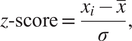 $$ z\hbox{-} \mathrm{score}=\frac{x_i-\overline{x}}{\sigma }, $$
where  $ \sigma $ and $ \overline{x} $ are the standard deviation and mean of the distribution of variable x, respectively, and $ {x}_i $ is the value of the variable $ x $ for the $ i $-th sample. It should be noted, however, that outlier detection methods based on simple statistical tools, like z-score, generally assume that the variables have normal distributions while neglecting the correlation between variables in a multivariate case.
The kNN is a 1050 algorithm for identifying anomalies in a dataset. The kNN method detects outliers by exploiting the relationship among neighborhoods in data points (Hautamaki et al., Reference Hautamaki, Karkkainen and Franti2004). The farther a data point is beyond its neighbors, the higher chance the data is an outlier. From a 1050 point of view, kNN is a supervised 1050 algorithm. However, when applied to outlier’s detection it takes an unsupervised approach, since the labeling of “outlier” or “not-outlier” in the dataset is entirely based upon threshold values. The  $ k $ number of neighbors to be considered is a parameter that needs to be specified.
2.1.2. Sampling
ML applications require datasets to be not only large but also balanced. This means that the number of instances (i.e., data points) for each class (e.g., a particular plant state) must be well distributed across classes (Ling and Li, Reference Ling and Li1998; Mohammed et al., Reference Mohammed, Rawashdeh and Abdullah2020). When this requirement is not met, two approaches can be taken: oversampling and undersampling. In oversampling, data augmentation methods are used to generate new datapoints, thus increasing the number of instances for a given class (Chawla et al., Reference Chawla, Bowyer, Hall and Kegelmeyer2002). In undersampling, not all the available instances for a given class are used to bring the number of instances of all classes to a similar level. In this work, we will focus on applications where large datasets are available and no oversampling is needed. Therefore, attention will be given to the effects of undersampling on data analysis and will be referred to as sampling hereafter. When sampling is needed, the ability of the sampled data to accurately represent the original data is of paramount importance. With this consideration in mind, we can identify three sampling procedures that aim, in some way or another, to provide a useful representation of the original data, but with fewer data points. The first approach is random sampling in which, after segmenting the complete dataset into intervals of equal size, a point is sampled at random from within each interval. The segmentation of the original dataset prevents regions of data from being overrepresented as each segment will have 1 representative point. Taking this idea further, the sampling and average method take the average of all points within each interval, thus including information from all points in each interval. These 2 methods sample equally along the dataset, which is acceptable if the data does not show rapid changes, or all the classes have approximately the same number of datapoints. In some applications, however, a method capable of identifying regions in the dataset where less data are needed (i.e., monotone regions) and regions where more data are needed (i.e., rapidly variable regions) might be preferred. A method based on the condensed Nearest Neighbor (cNN) algorithm is an example of such approach (Hart, Reference Hart1968). In cNN, data points that are similar are identified and classified. Using this information, the algorithm produces a reduced dataset in which the highly variable regions (that contain more classes) are more densely sampled.
2.1.3. Scaling
Most dimensionality reduction and clustering methods are sensitive to the relative magnitude of the variables included in the dataset. For example, in a chemical reactor 1 could have the vessel temperature being measured on the order of  $ 1\times {10}^2 $ while the exit concentration is being measured on the order of $ 1\times {10}^{-1} $. Such a difference in the magnitudes of the measured variables will cause the vessel temperature to overpower any appreciable observations associated with the exit concentrations, thus inducing errors in the data analysis. Among scaling methods, two main activities are defined: standardization and normalization. In standardization, a known probability distribution (e.g., a Gaussian distribution) is assumed for the data. The z-score method, previously discussed for outlier detection, falls into this category, as it is based on the probability of a score occurring within the normal distribution of the data. When applied for scaling, z-score enables us to compare two different scores that are from different normal distributions of the data.
In normalization, the assumption of a known probability distribution is removed, and the scaling is performed using estimators from the dataset itself. Methods such as over range, over min, and over mean are included in this category (García et al., Reference García, Luengo and Herrera2015). Over range, normalization is used to scale the data from 0 to 1. Over max or over min normalization is done by dividing the raw data by the maximum or minimum (minimum value must not be 0) values (Pedregosa et al., Reference Pedregosa, Varoquaux, Gramfort, Michel, Thirion, Grisel, Blondel, Prettenhofer, Weiss, Dubourg, Vanderplas, Passos, Cournapeau, Brucher, Perrot and Duchesnay2011). Over the mean normalization scales each variable on a 0 to 1 scale by dividing each value by the mean value of the variable. Finally, over min–max normalization performs a linear transformation on the original data (Han et al., Reference Han, Pei and Kamber2011). For a point  $ x $ the scaled value $ {x}_{scaled} $ using a min–max scaler is given by
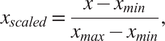 $$ {x}_{scaled}=\frac{x-{x}_{min}}{x_{max}-{x}_{min}}, $$
where  $ {x}_{min} $ and $ {x}_{max} $ are the minimum and maximum values of $ x $ in the dataset.
2.2. Dimensionality reduction
Dimensionality reduction is the process of reducing the number of variables or attributes under consideration. Generally, there are two major groups of dimensionality reduction methods: matrix factorization and neighbor graphs. In matrix factorization, the original high-dimensional space is decomposed as the product of two lower dimensional matrices and then an optimization algorithm is implemented to minimize the reconstruction error, obtained from the difference between the actual values in the original space and those computed from the product of the two matrices (Chiang et al., Reference Chiang, Russell and Braatz2000). In neighbor graphs, a mathematical graph is built in the high-dimensional space, that is, including all the variables, and then embedded in a lower dimensional space using a topological manifold (McInnes et al., Reference McInnes, Healy and Melville2018).
2.2.1. Matrix factorization
Among matrix factorization methods, one of the most widely used approaches is Principal Component Analysis (PCA). PCA focuses on models with latent variables based on linear-Gaussian distributions in which a set of orthogonal and uncorrelated vectors are found and ordered by the amount of variance explained in their directions (Chiang et al., Reference Chiang, Russell and Braatz2000). The latter is determined by solving the eigenvalue problem given as
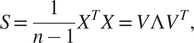 $$ S=\frac{1}{n-1}{X}^TX=V\Lambda {V}^T, $$
where  $ X\in {\unicode{x211D}}^{n\times m} $ is the matrix containing the observations in the original high-dimensional space, $ S $ is the sample covariance matrix, $ n $ is the number of observations, $ m $ is the number of variables, $ V\in {\unicode{x211D}}^{m\times m} $ is the matrix of loading vectors and $ \varLambda \in {\unicode{x211D}}^{m\times m} $ is the diagonal matrix containing the ordered non-negative real eigenvalues. The vectors corresponding to the largest singular values (the square of the eigenvalues) are typically retained and form a loading matrix, $ P\in {\unicode{x211D}}^{m\times a} $, where $ a $ is the number of singular values to be retained. The projection in the low-dimensional space is obtained as $ T= XP $ (Chiang et al., 2000). Because of the covariance analysis implicit in PCA, the method is limited to use only second-order information from the observed space and cannot incorporate prior knowledge. Several algorithms (kernel PCA (Lee et al., Reference Lee, Yoo, Choi, Vanrolleghem and Lee2004), probabilistic PCA (Kim and Lee, Reference Kim and Lee2003), multilinear PCA (Lu et al., Reference Lu, Plataniotis and Venetsanopoulos2006)) based on PCA have been developed to address these issues. Independent component analysis (ICA) is another matrix factorization technique in which the latent variables are assumed non-Gaussian and mutually independent. The components obtained are not orthogonal, and the observed variables (i.e., the original space) can be obtained as linear combinations of the latent space (i.e., the lower dimensional space). Thus, it requires higher order statistics to recover statistically independent signals from the observation of an unknown linear mixture. Due to these characteristics, ICA becomes useful for cases where PCA applicability is limited and higher order information must be included (Hyvärinen and Oja, Reference Hyvärinen and Oja2000; Cao et al., Reference Cao, Chua, Chong, Lee and Gu2003). Additional discussions on PCA variants can be found elsewhere (Gajjar et al., Reference Gajjar, Kulahci and Palazoglu2018; Lu et al., Reference Lu, Jiang, Gopaluni, Loewen and Braatz2018; Sundaramoorthy et al., Reference Sundaramoorthy, Varanasi, Huang, Ma, Zhang and Dian Wang2021).
2.2.2. Neighbor graphs
Neighbor graphs methods for dimensionality reduction generate a connected graph between the variables in the original high-dimensional space. Then, the algorithm looks for the topological manifold that minimizes the reconstruction error while preserving the relationship among the variables from the high-dimensional space to the low-dimensional embedding (McInnes et al., Reference McInnes, Healy and Melville2018). Two representative methods for the neighbor graphs approach are t-distributed stochastic neighbor embedding (t-SNE) (Maaten and Hinton, Reference Maaten and Hinton2008) and uniform manifold approximation and projection (UMAP) (McInnes et al., Reference McInnes, Healy and Melville2018). t-SNE works by converting the Euclidean distance between data points into conditional probabilities and tries to minimize the Kullback–Leibler (KL) divergence (Hershey and Olsen, Reference Hershey and Olsen2007) between the joint probabilities of the low-dimensional embedding and high-dimensional data (Joswiak et al., Reference Joswiak, Peng, Castillo and Chiang2019). The algorithm starts by computing the conditional probabilities  $ {P}_{ij} $ of xi “being a good neighbor” of $ {x}_j $, these are all the points from the original dataset $ {x}_1,\dots, {x}_n\in {\unicode{x211D}}^n $. The mathematical quantification of this idea is the probability:
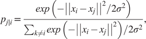 $$ {p}_{j\mid i}=\frac{\mathit{\exp}\left(-{\left|\left|{x}_i-{x}_j\right|\right|}^2/2{\sigma}^2\right)}{\sum_{k\ne i}\mathit{\exp}\left(-{\left|\left|{x}_i-{x}_j\right|\right|}^2\right)/2{\sigma}^2}, $$
where σ2 is the variance that represents the variability of the data with respect to its mean. Next, using a student t-distribution with 1 degree of freedom, a second set of probabilities ( $ {Q}_{ij} $) in the low-dimensional space is determined and given as
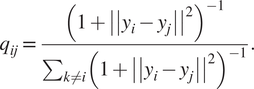 $$ {q}_{ij}=\frac{{\left(1+{\left|\left|{y}_i-{y}_j\right|\right|}^2\right)}^{-1}}{\sum_{k\ne i}{\left(1+{\left|\left|{y}_i-{y}_j\right|\right|}^2\right)}^{-1}}. $$
Finally, t-SNE optimizes over a set number of iterations, using gradient descent with Kullback–Leibler divergence as the cost function. The algorithm is stochastic, therefore, multiple executions with different random seeds will yield different results. It is acceptable to run the algorithm several times and pick the embedding with the lowest KL divergence. The KL divergence is defined as
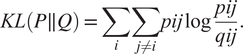 $$ KL\left(P\parallel Q\right)=\sum \limits_i\sum \limits_{j\ne i} pij\log \frac{pij}{qij}. $$
t-SNE is more accurate in preserving the local structure because the cost function is proportional to the joint probability in the high-dimensional space, hence, points that are relatively distant have a much lower impact on the cost function.
UMAP aims to find a transformation function for mapping high-dimensional data onto a low-dimensional plane. This is a clear distinction between t-SNE and UMAP as t-SNE directly optimizes an embedding. The steps for finding the transformation function are as followed: First, a weighted graph is computed for the high-dimensional data  $ {W}^H $ that models the local relationship of neighboring points. Second, a weighted graph is computed for a low-dimensional representation $ {W}^L $, similarly to the high-dimensional neighborhood. The low-dimensional representation is then determined by minimizing the cross entropy (McInnes et al., Reference McInnes, Healy and Melville2018), given by:
 $$ C\left({W}^H,{W}^L\right)=\sum_{i\ne j}{W}_{ij}^H\log \left(\frac{W_{ij}^H}{W_{ij}^L}\right)+\left(1-{W}_{ij}^h\right)\log \left(\frac{1-{W}_{ij}^H}{1-{W}_{ij}^l}\right). $$
By incorporating the second term in Eq. 7, the local relationships are also considered and preserved, in addition to the global relationships represented by the first term, which is also present in t-SNE(Eq. 6 above). As implemented by McInnes et al. (Reference McInnes, Healy and Melville2018), the most important hyperparameter for UMAP is the number of neighbors that are considered when constructing the weighted graph. Having a larger number of neighbors produces more global views of the structure, which preserves a more global structure of the data. Another important hyperparameter is the minimum distance between datapoints. A lower (or zero) minimum distance relaxes the constraints on the placement of the points in terms of the distance between neighbors. This typically leads to dense clumps of data. A large minimum distance typically leads to the datapoints being sparser in the low-dimensional plane.
2.3. Clustering
Clustering algorithms divide or partition data into natural groups. In our context, the notion of “natural” implies that the objects in a cluster should be internally similar to each other; but differ significantly from the objects in the other clusters (Tan et al., Reference Tan, Steinbach, Karpatne and Kumar2018).
One way of classifying clusters is as flat or hierarchical, based on the sequence the algorithm follows when forming the clusters. Flat clustering creates all clusters at the same time. Hierarchical clustering algorithms, on the other hand, find clusters one by one (Jain and Dubes, Reference Jain and Dubes1988). The hierarchical methods can be further divided into agglomerative and divisive algorithms, corresponding to bottom-up and top-down strategies. Agglomerative clustering algorithms merge clusters together one at a time to form a clustering tree which finally consists of a single cluster, the whole dataset. Divisive algorithms are similar but work in the opposite direction starting from a single cluster and dividing each cluster to sub-clusters until all vectors are in a cluster of their own (Jain and Dubes, Reference Jain and Dubes1988).
Clustering methods can also be classified as centroid-based or density-based, depending on how each cluster is built. Centroid-based clustering methods assumed a certain distribution within the clusters, and create new clusters around a point (i.e., a centroid) following this distribution. The number of clusters (centroids) is usually predefined, but it can also be part of an energy function (Buhmann and Kühnel, Reference Buhmann and Kühnel1993). In density-based clustering, no centroids are defined and no distribution of the data within the clusters is assumed. Density-based clusters are more versatile and powerful but require larger datasets to perform well (McInnes et al., Reference McInnes, Healy and Astels2017). In this discussion, focus will be made on two large groups of cluster methods: flat centroid-based, and hierarchical density-based.
2.3.1. Flat centroid-based clustering
Flat centroid-based clustering algorithms find the splitting of the dataset that minimizes the sum of the distance between the members of a cluster and the centroid of said cluster. In K-Means for example, K initial centroids are chosen corresponding to the number of clusters desired (the only hyperparameter for this method). Each point in the dataset is assigned to the closest centroid, and the centroid of each cluster is updated with each iteration based on the points assigned to the cluster (Thomas et al., Reference Thomas, Zhu and Romagnoli2018).
K-Means not only seeks spherical clusters in data (Tan et al., Reference Tan, Steinbach and Kumar2016), but it also clusters with roughly equal number of samples. Therefore, K-Means should never be blindly used to cluster any data without careful verification of the results. It should also be noted that as the number of clusters is increased, the number of samples in clusters decreases, which makes this algorithm more sensitive to outliers (Vesanto and Alhoniemi, Reference Vesanto and Alhoniemi2000).
Another flat centroid-based clustering method called Gaussian Mixture Models (GMM) treats the dataset as a combination of subsets, each of which is described by a gaussian distribution (Bishop, Reference Bishop2006). This provides a more flexible approach than that of K-means by assigning a measure of uncertainty to the assignment of a point to a particular cluster. However, the disadvantages of flat clustering, as will be described in the next section, are still present.
2.3.2. Hierarchical density-based clustering
Given a measure of proximity, density-based clustering looks for clusters of any shape and without need of initial centroids or the assumption of equal variables around a point (Gaussian sphere assumption). Furthermore, density-based clustering does not require every data point to be assigned to a cluster, allowing for data in sparse regions to be identified as noise. These features provide an advantage over partitional clustering, since fewer assumptions are made regarding the distribution of the data, which can become important when dealing with high-dimensional data (McInnes et al., Reference McInnes, Healy and Astels2017). A representative example of density-based clustering algorithms is density-based spatial clustering of applications with noise (DBSCAN) (Ester et al., Reference Ester, Kriegel, Sander and Xu1996). To deploy DBSCAN, two hyperparameters are needed: epsilon (eps), the radius of a neighborhood; and min_samples, the minimum number of points within the neighborhood radius of a point for such point to be considered a density point.
Defining the number of clusters to be obtained (a prerequisite for K-Means, for example) can be difficult when little is known about the real distribution of the data in the high-dimensional space. In this scenario, the notion of further divided clusters preserving the hierarchical relationship among them has proved to be useful. Such is the case of clustering algorithms such as hierarchical density-based spatial clustering of applications with noise (HDBSCAN), which uses hierarchical clustering to improve the density-based approach provided by DBSCAN (McInnes et al., Reference McInnes, Healy and Astels2017). In terms of implementation, this means that the eps hyperparameter for DBSCAN is no longer required to be input manually; but is rather learned from the clustering algorithm. This allows for clusters with different densities, which could be desired for higher resolution.
2.3.3. Clustering analysis: subspace greedy search
Once the dimensionality reduction and clustering procedures are performed, further analysis of the resulting clusters could be needed to extract meaningful conclusions. Subspace greedy search (SGS) is an algorithm that allows for the identification of the variables responsible for the separation between 2 given clusters. To do this, SGS starts by analyzing the lowest dimension, then moves to higher dimensions until no possible subspaces are left. The k-nearest neighbor distance (k-distance) between the clusters for each subspace is used as a score to compare the different subspaces that contain the same dimension. The lower scores are discarded and the highest move on to further analysis. The basic idea is inspired by Micenkova’s concept of explanatory subspace (Micenková et al., Reference Micenková, Ng, Dang and Assent2013), which characterizes differences between clusters by greedy searching for the most contributing combination of variables. The implementation of a greedy algorithm dramatically reduces the computational cost for searching the target combination of variables, which allows such algorithm to be implemented in real-time scenarios for fault diagnosis. A detailed description and implementation of SGS can be found elsewhere (Zhu et al., Reference Zhu, Sun and Romagnoli2018).
2.4. Data visualization: self-organizing maps
Parallel to dimensionality reduction and clustering, other 1050 tools could be implemented for pattern recognition and data visualization. A self-organizing map (SOM), also known as a Kohonen network, is a neural network used to visualize complicated, high-dimensional data (Kohonen and Somervuo, Reference Kohonen and Somervuo2002). A SOM is described formally as a nonlinear, ordered, smooth mapping of high-dimensional input data manifolds onto the elements of a regular, low-dimensional array, and is therefore a method to do dimensionality reduction. It simultaneously performs vector quantization and topographical preservation while representing complex multivariate data on a two-dimensional grid (Kohonen, Reference Kohonen1995).
The visualization abilities of SOM are extremely helpful for the preprocessing of unlabeled plant data and viewing the clustering structure of a dataset. A SOM consists of components called nodes or neurons. Each node is associated with a weight vector of the same dimension as the input data vectors, and a position in the map space. From the weight vector, a corresponding map for each of the variables can be extracted (component maps), which allows the identification of correlations between the components and the overall distribution of the data. The nature of the SOM makes it possible to be utilized for various industrial applications, such as data visualization, process monitoring, etc. (Ge et al., Reference Ge, Song, Ding and Huang2017). Since SOM can cluster data without knowing the class memberships of the input data, features inherent to the problem can be detected (Alhoniemi et al., Reference Alhoniemi, Hollmén, Simula and Vesanto1999). Because the SOM algorithm performs a topology-preserving mapping from high-dimensional space onto map units, relative distances between data points are preserved. This latter characteristic enables generalization, that is, the network can interpolate between previously encountered inputs (Kohonen, Reference Kohonen2012).
As described in Section 2, the DMKD workflow involves making a number of decisions regarding the methods to be used and the corresponding hyperparameters. In the following sections, an exploration of how these decisions influence the overall analysis is presented. First, a user-friendly graphic interface for easy DMKD analysis is described. Then, different methods are implemented on simulated data, where the actual patterns in the plant are known, to investigate the methods’ ability to detect such patterns. Lastly, real industrial data is used to showcase the intricacies of implementing DMKD in real life settings.
3. Materials and Methods
3.1. Data analysis environment
A Python-based data analysis graphical user interface, called FastMan (Fast Manual data classification), was developed using Python libraries (NumPy, pandas, sci-kit learn, etc.) to facilitate the use and manipulation of different methods for data preprocessing, dimensionality reduction, clustering, and cluster analysis. The data analysis methods available in FastMan are summarized in Table 1. FastMan asks the user to select a method for each step of the DMKD methodology, moving from left to right in Table 1. The user interface also allows to go back at any point and change the method selection. It is worth noting that although not all the methods available in FastMan are demonstrated in this work, a brief review of their main characteristics is provided for the reader to have a context of the different ways data mining for chemical process applications could be conducted.
Table 1. Data preprocessing and analysis methods available in FastMan.
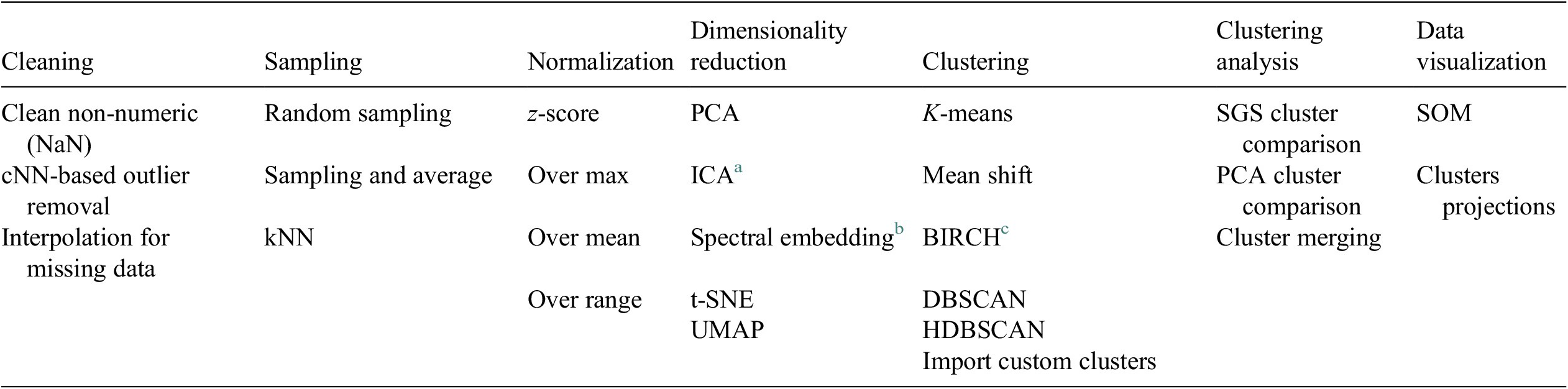
a Independent component analysis (Hyvärinen and Oja, Reference Hyvärinen and Oja2000).
b Laplacian eigenmaps (Belkin and Niyogi, Reference Belkin and Niyogi2003).
c Balanced iterative reducing and clustering using hierarchies (Zhang et al., Reference Zhang, Ramakrishnan and Livny1996).
Figure 2 shows an example of a typical view of FastMan. Line plots of the process variables are shown in the top-center panel of the window, where multiple plots can be extracted for a better visualization using a contextual menu on the bottom-center panel. The top-left panel allows selection of the data analysis methods as the user navigates the typical data mining process (cleaning-sampling-normalization-dimensionality reduction-clustering) using the arrows over the panel. The bottom-left panel prints out information about the state of the current operation. The top-right panel shows the data visualization output using dimensionality reduction and clustering or SOM. On the bottom-right, the user can select which clusters to visualize as well as perform operations for clustering analysis such as cluster merging and comparison using a contextual menu. In addition to the visualization of data mining results, FastMan enables saving the results as single or multiple files for further analysis and use in a supervised learning environment.
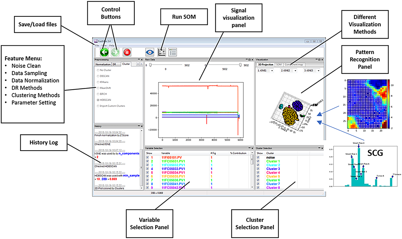
Figure 2. FastMan typical view.
3.2. Simulation and data collection
When simulated data was used, the overall process model was implemented in the Aspen HYSYS® simulation environment and data from the simulations were extracted using an in-house Python-based tool to create scenarios and collect data.
4. Results and Discussion
Results are presented for two case studies: a simulation example and an industrial case study. As stated before, the use of simulated data allows for verification of findings while the use of real data shows the applicability of these methods in real-life scenarios. Figures have been converted to grayscale format for purpose of editorial printing. However, color images will be available in the additional material and will allow the reader a clearer visualization of the concepts discussed in the paper.
4.1. Case study 1: Natural gas liquids (NGL) simulated plant
4.1.1. Process description
Figure 3 shows a schematic representation of the Natural gas liquids (NGL) process. The recovered raw gas feed is cooled to −4.8 °C by a gas–gas heat-exchanger (E-100) and then further cooled by a chiller (E-101) to reach an appropriate temperature for the separation of condensates in a flash separator (TK-100). The gas stream leaving the separator (TK-100) is further cooled by the gas–gas heat-exchanger (E-102). Both the cooled gas and condensates are fed to the demethanizer column (T-100) at different feed locations. More details of the process are given by Zhu et al. (Reference Zhu, Chebeir and Romagnoli2020). Three types of scenarios were used to generate datasets. At t=1200 a step change in the feed composition was introduced to generate a global disturbance and at t=3,500 and t=5,500 two additional steps changes in the pressure setpoint (PIC-100) and bottoms’ composition setpoint (XIC-100) were introduced to generate local disturbances. The total dataset included 7,726 points for 62 process variables.
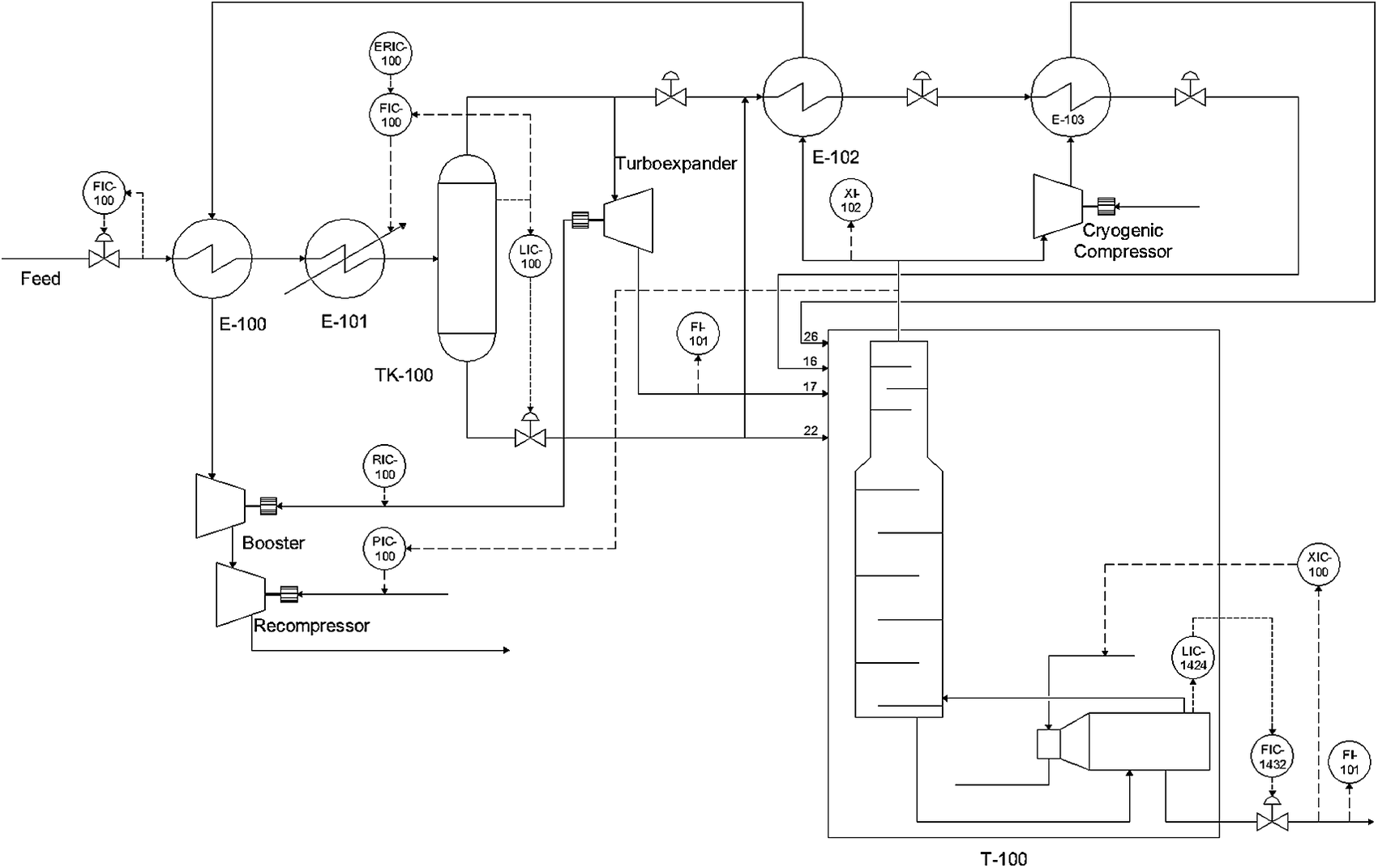
Figure 3. Simulated NGL plant schematic (Chebeir et al., Reference Chebeir, Salas and Romagnoli2019).
4.1.2. Data preprocessing
Since the data used in this case study comes from a simulation, no outliers or measurement noise is expected. Therefore, the data cleaning step only included a screening for non-numerical values and missing data. In this application, the focus of the preprocessing will be on analyzing the effect of scaling/normalization of the original data set. Two scaling methods (over max, over mean) and one normalization method (z-score) were compared and visualized using SOM to quantify the effect on final data classification.
Figure 4 (left) shows the temporal variations of XIC-100.PV process variable (chosen as indicator) through the different scenarios discussed before. It can be observed that from an undisturbed initial condition the plant evolves through different changes and operational statuses. Overall, we can identify four operational conditions including the starting point. Figure 4 (right) illustrates the characterized process conditions within the SOM plot using z-scores as normalization approach.
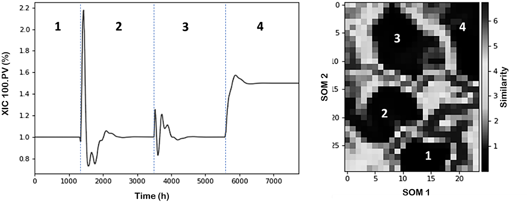
Figure 4. NGL time evolution of XIC 100.PV variable and partition of operational conditions. (Left) Line plot. (Right) SOM (Darker regions represent high similarity (clusters) between datapoints, and brighter regions represent low similarity (separation between clusters)).
4.1.2.1. Effect of sampling
The effect of sampling was investigated using random sampling and cNN. Data were normalized using z-score in all cases. Figure 5 illustrates the sampling effect visualized as SOM, 3D projection (using PCA-DBSCAN), and time evolution of XIC 100.PV. Using random sampling (first row) the data size is reduced by approximately six fold, from 7700 to1400 data points, however, this reduction does not affect the quality of the dataset and the analysis since the main events are still captured as indicated by the corresponding SOM, 3D projection and temporal variation of XIC 100.PV. Four main clusters are identified and properly classified using PCA-DBSCAN. In the case of cNN approach, the same reduction is obtained, however, clearly some of the events captured in the original data set are lost, as indicated by the corresponding plot. The SOM features are completely modified and only two main clusters are identified by the PCA-DBSCAN combination. Some of the main dynamics of the XIC 100.PV variable, including the stability reached after the changes by action of the controllers, are lost. This observation is consistent with the main feature of cNN which is to reduce the amount of data points in monotone regions (stability) and to keep more data points in highly variable regions.

Figure 5. Effect of sampling on the visualization and classification for the NGL plant via SOM, 3D projection, and time evolution of XIC 100.PV process variable. First row shows random sampling and second row shows cNN sampling.
4.1.2.2. Scaling/normalization
Figure 6 illustrates the results comparing alternative scaling/normalization approaches: z-scores (first row) and over mean (second row). From these results, it is evident that the scaling/normalization method has a strong influence on the visualization of the process conditions through the SOM. Furthermore, the use of SOM with z-scores is able to characterize the process operating conditions (brighter separation among operating status). When using over mean, on the other hand, the separation between the clusters becomes less clear (darker boundaries between the clusters).
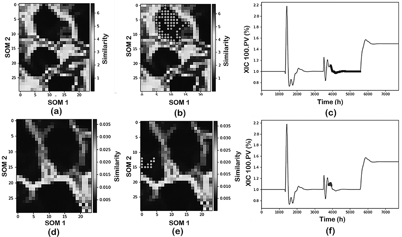
Figure 6. Effect of scaling over the visualization and projections of process data from the NGL plant: (first row) z-score and (second row) over mean.
Since the SOM visualization is just one component of the data mining tools, the implications of the scaling/normalization on the data classification are also analyzed. Figure 6b,c,e,f shows the projection of one of the operating conditions (pressure change) as identified by the DR-Clustering into the SOM and into the time evolution for the two approaches. In this case, the combination of PCA-DBSCAN (min_sample = 60) as DR and clustering tools is utilized. As shown in the figure, the z-score normalization in combination with the PCA-DBSCAN perfectly captures the operating condition identified previously both in the SOM representation and the time projection. Meanwhile, using over mean scaling, the PCA-DBSCAN combination characterizes an additional operating status of the plant subdividing the pressure change into two separate clusters.
From the previous discussion, it becomes clear that the scaling/normalization approach used has strong implications for the data visualization as well as classification. It should be noted that some of the results provided above for classification can be shaped accordingly using alternative DR/clustering tools as well as proper adjustment of the hyperparameters involved. However, in the case of industrial data where no previous knowledge of the operating status of the plant is known, this is not possible without a proper visualization approach as provided by SOM as will be discussed later in the industrial application case study.
4.1.3. Data analysis and classification
After the analysis of preprocessing techniques, focus shifted to extracting information from the given data set. As illustrated in Figure 4, the data set for the NGL plant contains information on four main operating conditions due to effect of disturbances and set-point changes. Consequently, one of the tasks of data mining is to be able to characterize the different plant statuses and classify the data accordingly.
4.1.3.1. Effect of DR techniques
Figure 7 shows the comparisons using PCA, t-SNE, and UMAP in terms of the 3D clusters plot, SOM projection and time evolution of the XIC 100.PV with data projected according to region 2. In this analysis a reduced set data was used (random sampling, sampling = 5) and DBSCAN as clustering technique. PCA-DBSCAN (min_samples = 20); t-SNE-DBSCAN and UMAP-DBSCAN (min_samples = 50) were used respectively.
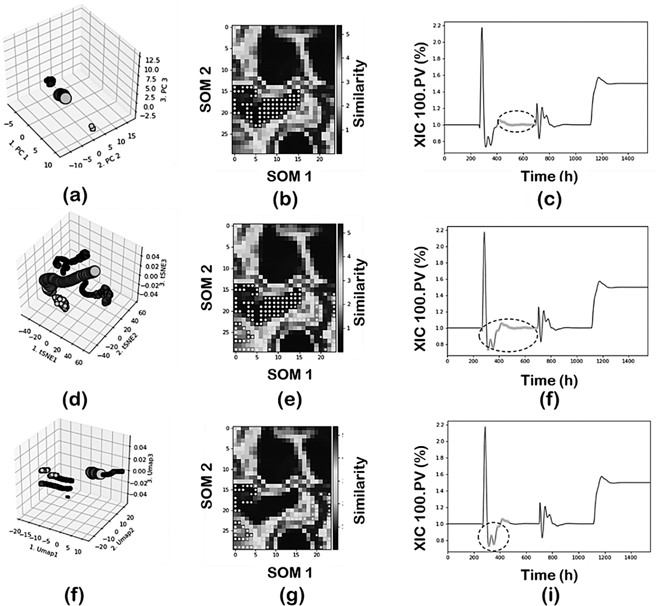
Figure 7. Effect of DR techniques: (first row) PCA; (second row) t-SNE; and (third row) UMAP.
The PC-DBSCAN combination can identify the four regions, leading to a perfect classification of the data according to the main operating conditions of the plant. The use of t-SNE or UMAP as DR techniques leads to an increased number of clusters in the final classification since they tend to capture not just the main operating conditions but also to capture the transient states dynamics due to the control actions. In the case of t-SNE for region 2, part of the transition data is added to the specific cluster and in the case of UMAP the region is further decomposed as shown in Figure 7h. This means both t-SNE or UMAP as DR techniques provide more resolution when analyzing the data and are able to capture not just the global effects (main changes in operating conditions where most variables are involved) but also local effects (few variables are involved). This main difference between PCA and the neighbors graph approaches (t-SNE and UMAP) has important implications in real operations where those changes may last for several hours which in a large dataset may represent just a local effect. Furthermore, it is important to note the separability properties of the neighbor’s graph approaches. Projections of the regions are farther distanced as compared to the PCA projection. The effect of min_sample parameter will be discussed separately.
4.1.3.2. Effect of clustering techniques
Figure 8 shows the application of PCA as DR with alternative clustering techniques, DBSCAN, HDBSCAN (min_samples= 50 for both), and K-Means (k = 4) to the data set. In general, HDBSCAN adds an additional level of resolution to the analysis as compared to DBSCAN. The combination PCA-DBSCAN strictly captures the new state, and the transient is added to the noise component (cluster). PCA-HDBSCAN on the other hand reduces the level of noise and captures part of the transient into the main cluster. That is, the level of noise captured by HDBSCAN is reduced significantly since other transitions were classified as part of the main clusters. This is 1 of the nice features of density-based clustering as it can classify some of the data points as noise. Typically, most transitions between operations are classified as noise when the PCA-DBSCAN combination is used and the size of the noise cluster is reduced in the case t-SNE and UMAP, since some of the transitions are captured as main clusters.

Figure 8. Effect of alternative clustering techniques: (a-c) DBSCAN; (d-f) HDBSCAN; and (g-i) K-Means.
The use of K-Means in this application does not produce a good separation since it lumps conditions 3 and 4 into a single cluster, and an additional cluster is created representing the dynamic between conditions 1 and 2.
4.1.3.3. Effect of min_sample
The final number of clusters, and therefore the resolution of the pattern, also depends on the selection of the hyperparameters for the clustering algorithm. Although the selection of the right hyperparameters will depend on each specific application and any domain knowledge the analyst may have, an overview of their effect on the result is provided here as a general guide. In our analysis, the parameter used to “adjust” the number of clusters in each approach was min_samples in the clustering methods. The default values in FastMan for the eps (epsilon radius parameter) are calculated from the data structure using K-Nearest Neighbors algorithm. As a basic simple rule, increasing the min_samples decreases the number of clusters and some of the clusters are merged. For example, part of the transient operation may be added to the new state cluster. Default value for min-samples parameter in FastMan is 10.
Figure 9 illustrates the results when min_samples in a PCA-DBSCAN combination is decreased to 10 and then to 5, and its effect on classifying region 2. First, decreasing from 50, as used before (Figure 8b,c), to 10 maintains the same number of clusters but the cluster representing region 2 is now capturing part of the transient state (Figure 9a,b). Furthermore, reducing the min_samples to 5 increases the number of clusters subdividing the original region. The new cluster captures part of the transient component between the two regions and consequently, the size of the noise cluster is reduced by lowering the min_samples parameter. An interesting feature of FastMan is the possibility of merging clusters manually. This is a very important feature, especially when dealing with industrial data and if the goal is to classify the data for future supervised learning approaches for pattern recognition. One can use the powerful visualization features of SOM to manually adjust the clusters to reduce the number of clusters to match the operating regimes characterized by SOM without the need to tune the hyperparameters.
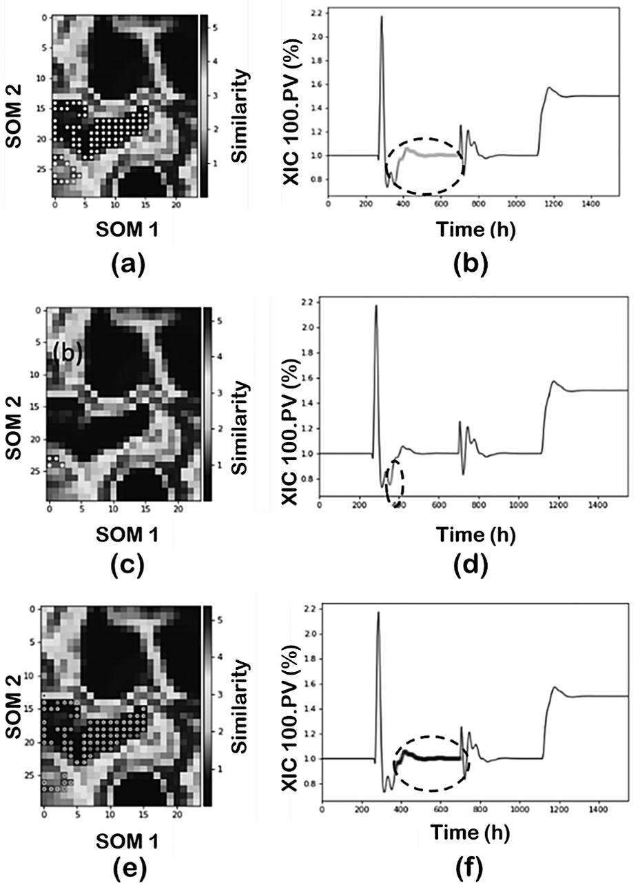
Figure 9. Effect of min_samples parameter: (a, b) min_samples = 10 and (c-f) min_samples = 5.
4.1.3.4. Cluster analysis
Using the clustering results from t-SNE and DBSCAN, a subspace greedy search analysis was conducted to assess the DMKD implementation’s ability to correctly identify the variables responsible for the patterns observed in the data. Figure 10(left) shows the results from the SGS analyses between clusters 3 and 4 (XIC 100 set-point change). The SGS analysis was able to find the correct variables associated with the changes. In addition to the distance matrix visualization of the SOM already shown in our discussions, a component analysis was conducted. In the component analysis using SOM, the contributions of each variable to the clustering results are projected in individual maps. This information complements and verifies the results from the SGS analysis. Figure 10(right) shows the SOM component projections for the most contributing variable to the cluster distributions by the SGS. Accordingly, the SOM component projection for each of the most influential variables (in this case the XIC 100.PV) matches perfectly the shape of the corresponding region in the overall SOM (right upper corner).

Figure 10. Cluster analysis results: (left) SGS analysis of the clusters produced with PCA-DBSCAN combination. (right) Cluster projections over the components SOM for most influential variable.
4.2. Case study 2: Industrial pyrolysis reactor
4.2.1. Process description
The pyrolysis reactor is an important unit in the chemical industry used to crack heavier hydrocarbons to lower molecular weight hydrocarbons. The entire reactor is placed in a fired furnace, where the energy required for the reaction is generated from fuel gas combustion. In this study, the data come from an industrial scale furnace reactor, in which naphtha is cracked to ethylene. As shown in Figure 11, six coils of naphtha are mixed with steam before cracking in the furnace. The ethylene product is generated by cracking the mixture through the furnace at a high temperature (around 1000 °C). 27 variables are utilized for process monitoring, involving mainly hydrocarbon and steam process flows and fluid temperatures entering and leaving the combustion chamber. A more detailed description of the system be found in Zhu et al. (Reference Zhu, Webb, Mao and Romagnoli2019).

Figure 11. Schematic representation of the industrial pyrolysis reactor.
4.2.2. Data preprocessing
4.2.2.1. Data cleaning and outlier removal
Real plant data often contains outliers and erroneous data, and it is of interest to have a method to detect and remove such data points to minimize the effect on the overall analysis. However, caution is required when dealing with outliers. As shown in Figure 12, what at first glance might be considered an outlier, actually represents a large variation of the total hydrocarbon flow for about 5 hr of operation. This period represents a small portion of the data thus the corresponding set of data is categorized as outliers (does not conform to the main data distribution) and adjusted accordingly. Therefore, an outlier detection and removal method that can distinguish between rare operation states and true outliers is desired. In FastMan, outliers are detected using the kNN algorithm. However, to prevent the loss of meaningful information, the outliers are not deleted but rather labeled.

Figure 12. Rare operation states in the pyrolisis reactor dataset. (a) raw data; (b) zoom around apparent outlier; and (c) further zoom showing a 5 hr operation region.
Figure 13 illustrates the case of the same situation now in the measurements of hydrocarbon flows in coils 2 and 6. In Figure 13d, a projection of the data is also given using the projection tools discussed before to illustrate the effect of the outliers in data analytics. The encircled region in Figure 13d corresponds to the outliers which are clearly well separated from the main data distribution. A combination of PCA and DBSCAN for dimensionality reduction and clustering were used, respectively. In this case, it is not a single outlier but several points that create a new cluster. The number of k-neighbors, the single parameter required for kNN, strongly influences the amount of data being classified as outliers. By increasing the number of neighbors, more data points are designated as anomalies, leaving only important features in the final dataset. However, for a given dataset, the point of diminishing returns will be reached at some value of  $ k $. As shown in Figure 14, for this specific example increasing the number of neighbors beyond $ k=50 $ does not improve the data substantially.

Figure 13. Hydrocarbon flows for coils 2 and 6 for pyrolysis reactor: (a) raw data; (b) data after outliers’ detection/elimination; (c) zoomed view of the section within the circle; and (d) data projected in a 3D space using PCA-DBSCAN.

Figure 14. Effect of number of neighbors,  $ k $, over the data makeup for the pyrolysis reactor.
4.2.2.2. Sampling
The effect of sampling real plant data was investigated using random sampling and cNN with different values of  $ k $. Data were normalized using z-score in all cases. Figures 15 and 16 illustrate the sampling effect on 2 of the process variables (steam flow in coils 2 and 5). Figure 15 shows the results for the cNN sampling approach with k number of neighbors 5 and 50. Both the time evolution of the variables and the associated 3D projection (using PCA-DBSCAN combination) are given. For the cNN approach the data size is reduced sixfold, from7800 to 1400 data points, however, this reduction does not affect the quality of the dataset since the main events are still captured in any of the 3 conditions investigated. This is shown with the help of 3D projection plots which clearly illustrate 3 main events captured by the data. The number of neighbors slightly changes the size of the data but does not have further influence on the analytics. This agrees which the idea that in this approach the highly variable regions (more classes) are more densely sampled. Furthermore, since no steady state is actually reached (real plant conditions and the drifting nature of the pyrolysis reactor) the effect of cNN is different from that observed with simulated data.
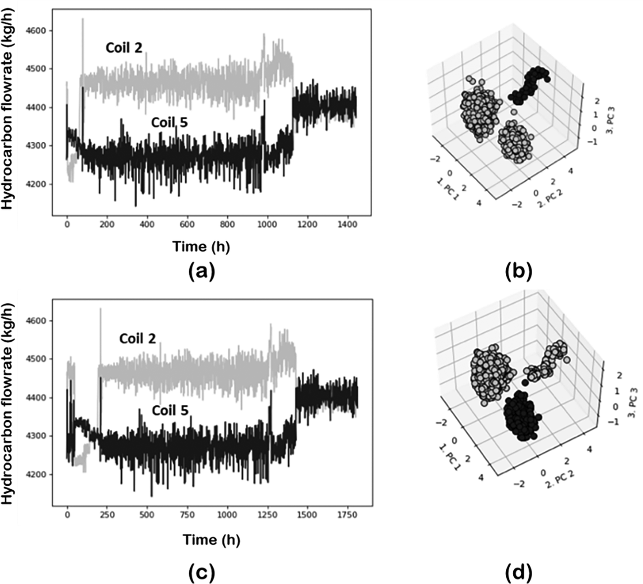
Figure 15. Effect of sampling on the process variables. cNN sampling: (a) k = 5 and (c) k = 50. (b) and (d) corresponding projection to 3D space.

Figure 16. Effect of sampling on the process variables. Random sampling: (a) n = 2 and (c) n = 10; (b) and (d) corresponding projection to 3D space.
Figure 16 shows the results for the random sampling strategy with interval values of 2 and 10. Data have been reduced from 7800 data points to 3500 and 1400 respectively. In this case, some of the events captured in the original data set are lost to some degree, depending on the size of the interval. The event occurring at the start of the operation is lost (for n = 10) or not captured completely (n = 2). In the latter cases, the original region is subdivided into two smaller regions, according to the 3D projection.
4.2.3. Data analysis and classification
Figure 17 illustrates the time evolution of the steam flows for coils 2 and 5 and hydrocarbon flows for coils 1 and 5, respectively. The analysis was done on the total set of measurements but for simplicity, we will focus our discussion on these four flowrates. The projection plots and the SOM are illustrated in Figure 18 (the line arrow indicates time direction of the batch).

Figure 17. Process variables time evolution: (a) coils 2 and 4 steam flow rates and (b) coils 1 and 5 hydrocarbon flowrates.

Figure 18. Process variables time evolution:(a) 3D projection plots and (b) the SOM for the PCA-DBSCAN.
Figure 19 illustrates the projection of the main cluster identified by PCA-DBSCAN into the time evolution and the SOM. Using this combination, most of the operating cycle is characterized as a single cluster. However, as observed in the SOM, a number of subregions are present (light colors separations) throughout the cycle.

Figure 19. Projection of the main cluster as predicted by PCS-DBSCAN into SOM: (a) time evolution plot and (b) SOM.
Figure 20 shows the results when the min_samples parameter in DBSCAN is reduced from 10 to 5. In this case, the methodology identifies an additional region in the top right corner of the SOM as well some additional regions in the startup and shut down conditions. The figure illustrates the projections of these two main clusters on the time evolution plot and the SOM (Figure 20a,b,d,e). Next, the analysis of formation of these two clusters is performed and illustrated in Figure 20c,f in terms of the component map and SGS contributions plot, respectively. As shown in Figure 20c, the component map for coil 5 steam flowrate is the main contributor to the cluster formation since the component map perfectly matches the overall SOM features. This is corroborated through the contributions plot, where the main contributors are the steam flowrates and in particular steam flowrates of coils 1 and 5. This can also be inferred from the time evolution plot in Figure 20d where a sharp increase/decrease in these flowrates can be observed.

Figure 20. Projection of clusters when min_sample in DBSCAN is reduced from 10 to 5: (a, d) time evolution plot; (b, c, e) cluster projection over the SOM; and (c) subspace greedy search results.
Similar analysis was performed using a neighbor’s graph approach and clustering (in this case the t-SNE-DBSCAN eps 6; min_samples = 80) to compare the results of feature extraction. Figure 21a illustrates the time evolution of the hydrocarbon flows of coils 1 and 5. Dotted boxes identify the operating regions identified by the DR and clustering combination of t-SNE-DBSCAN. The clustering results are given in Figure 21b. In this case, t-SNE projects the data into a 2D space. Five main clusters are clearly identified and also indicated in the time evolution plots. As can be seen, the large cluster identified previously using PCA is now subdivided into four subregions showcasing the better resolution of t-SNE. These subregions were also present in the SOM plot as discussed before (although not identified using PCA projection) and correspond to local system behavior (a small number of variables change significantly), as compared to the global changes discussed previously, for sharp changes in the steam flows. Figure 22 illustrates the cluster (corresponding to 2 subregions) projected into the time evolution as well as into the SOM and component plots. In this specific case, the most contributing variables are coils 1 and 5 hydrocarbon flow rates (Figure 23).
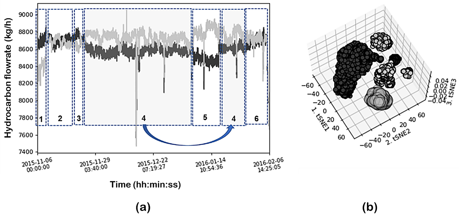
Figure 21. (a) Time evolution of the hydrocarbon flows of coils 1 and 5. Circles identify the operating regions identified by the DR and clustering combination of t-SNE-DBSCAN; (b) clustering results in 3D plot.

Figure 22. Cluster (corresponding to two subregions) projected into the time evolution as well as into the SOM and component plots.

Figure 23. Contributing variables as identified by the subspace greedy search. Variables with the highest scores have a greater influence on the distribution of the data (i.e., cluster separation).
5. Conclusions and Recommendations
A computational environment was used for data mining and knowledge discovery with both simulated and real plant data to demonstrate the applicability of DMKD for chemical processes analysis, as well as how the result is affected by the method selection and hyperparameters used.
For the preprocessing stage of DMKD, outlier detection and removal, scaling and sampling greatly affect the subsequent analysis and could dramatically change the interpretation of the results. For outlier removal, the effect of the number of neighbors used with kNN was shown. Also, the special consideration of rare operation states was illustrated. For sampling, it was demonstrated that cNN outperforms random sampling for real plant data but might cause loss of information when long periods of steady-state operation are present. Finally, for scaling, standardization using z-score was demonstrated to outperform normalization strategies.
Dimensionality reduction and clustering algorithms successfully identified changes and different operation states in both real and simulated data. However, neighbor graphs dimensionality reduction methods such as t-SNE and UMAP were shown to better identify global and local changes in the process than matrix factorization methods like PCA. Comparing t-SNE and UMAP, we can conclude from our analysis that both techniques are similar in their visualization capabilities, however, UMAP has a clear advantage over t-SNE in runtime. While both UMAP and t-SNE produce somewhat similar output, the increased speed and better preservation of global structure make UMAP a more effective tool for visualizing high-dimensional chemical processes data. Furthermore, once a model has been created using the historical information, incoming data points can be passed through the same UMAP model for on-line process monitoring and fault detection systems (Kohonen, Reference Kohonen1995).
In terms of clustering, hierarchical density-based clustering techniques have shown superior performance over flat centroid-based clustering in dealing with chemical process data. HDBSCAN adds an additional level of resolution to the analysis as compared to DBSCAN. In most of our results, DBSCAN strictly captures the new state, and the transient is added to the noise component (cluster). HDBSCAN on the other hand reduces the level of noise and captures part of the transient into the main cluster. In general, neighbor graphs dimensionality reduction methods have been shown to capture local and global events, the combination of either t-SNE or UMAP with DBSCAN provides a good compromise in terms of the level of resolution and reducing the number of clusters.
SGS was employed to identify the variables responsible for the distribution of the data. SGS effectivity was demonstrated using simulated data (real changes are known), where the algorithm successfully identified the correct variables as the main drivers for the observed changes. A similar analysis was conducted using the real data from the pyrolysis reactor to show the applicability of SGS for real industrial scenarios.
SOM was used for data visualization and clustering verification. The capabilities of SOM for detecting patterns in the data as well as identifying correlations between each of the original variables and the overall distribution of the data. Hence, it is recommended to include SOM analysis for DMKD implementations to complement the observations derived from dimensionality reduction and clustering.
Finally, FastMan, a friendly graphic interface for data mining and knowledge discovery was presented. The computational framework can be used with any dataset and facilitates the combination of several data preprocessing, dimensionality reduction, and clustering methods, as well as the visualization of the results.
Data Availability Statement
Data that support the findings are available from the authors (jose@lsu.edu). Restrictions apply to the availability of real plant data which were used under license for this study.
Author Contributions
Conceptualization: L.A.B., M.N., M.G.B., J.A.R.; Data curation: L.A.B., M.N., J.A.R.; Investigation: L.A.B., M.N., M.G.B., J.A.R.; Methodology: L.A.B., M.N., M.G.B., J.A.R.; Project administration: J.A.R.; Resources: J.A.R.; Supervision: J.A.R; Visualization: L.A.B., M.N., J.A.R.; Writing—original draft: L.A.B., M.N., M.G.B., J.A.R.; Writing—review & editing: L.A.B., M.N., M.G.B., J.A.R.
Funding Statement
This work received no specific grant from any funding agency, commercial or not-for-profit sectors.
Competing Interests
The authors declare no competing interests exist.


 Open access
Comments
No Comments have been published for this article.