


Impact Statement
It is shown in this paper that industrial assets with low amount of data can significantly improve the performances of their anomaly detection classifiers by collaborating with similar assets containing more data. The proposed technique enables collaborative learning via a hierarchical model of the asset fleet, where the higher level distributions represent the general behavior of asset clusters and individual asset level parameters sampled from the higher level distributions.
1. Introduction
Modern industrial asset operations are monitored in real time using a plethora of embedded sensors. Availability of asset condition time series combined with readily available computing power and communication technologies has extensively automated industrial operations in the recent decade (Xu et al., Reference Xu, He and Li2014; Gilchrist and Gilchrist, Reference Gilchrist and Gilchrist2016).
Asset health management, in particular, has moved from physics-based formulations to machine learning (ML) techniques. As a part of asset health management, detecting anomalies in an asset’s condition data is critical for accurate prognosis. An ideal anomaly detection algorithm instantaneously identifies deviations in real time, and activates the prognosis algorithm to plan timely maintenance. Accurate anomaly detection also enables efficient extraction of the failure trajectories from historical condition data. Failure trajectories are the time series ranging from the asset’s deviation from normal behavior till its failure. Since historical failure trajectories constitute the training dataset for prognosis, learning capabilities of the prognosis models primarily depend on accurate anomaly detection. An inefficient anomaly detection algorithm instead could let a failure go undetected, or flag many anomalies that turn out to be benign and not require any intervention (Kang, Reference Kang2018).
Most industries rely on rule-based systems for anomaly detection. These comprise of preset warnings and trip limits on the sensor measurements (Saxena et al., Reference Saxena, Goebel, Simon and Eklund2008; Zaidan et al., Reference Zaidan, Harrison, Mills and Fleming2015). Force tripping an asset often results in production losses, which could have been avoided if a planned maintenance was carried out in good time. Moreover, the warning-trip systems are inherently nonresponsive. An asset, for example, could not only be operating well within the limits, but also be deviating from its normal behavior. This deviation would not be flagged by a warning-trip system until sensor measurements exceedd the preset limits, which could already be too late and the opportune time be lost.
In scenarios where the domain knowledge about the underlying distribution is available beforehand, statistical classifiers provide a justifiable solution for anomaly detection. Statistical classifiers posit that the condition monitoring data generated during normal asset operations can be described using underlying distributions. Assuming that an asset commences operating in normal condition, the underlying density function  $ p\left(\theta \right) $, $ \theta $ being its parameters, can be estimated to model that asset’s normal operation data. Upcoming anomalies in asset operations cause a change in system dynamics, and induce deviation from its estimated density function. Statistical tests are used to evaluate if a newly recorded data point is significantly different to be deemed anomalous (Rajabzadeh et al., Reference Rajabzadeh, Rezaie and Amindavar2016; Kang, Reference Kang2018).
Statistical classifiers are among the recommended anomaly detection techniques in the recent literature on asset health management (Kang, Reference Kang2018). The asset condition data are associated with intrinsic and extrinsic measurement errors caused by system instabilities and inefficiencies, even while the asset is operating in stable conditions. For most preliminary algorithms deployment and simulations, the combined random effect of error and fluctuations in the sensor measurements has been treated as multivariate Gaussian (Kobayashi and Simon, Reference Kobayashi and Simon2005; Saxena et al., Reference Saxena, Goebel, Simon and Eklund2008; Borguet and Léonard, Reference Borguet and Léonard2009).
But independent modeling of assets is accompanied with challenges, primarily those of distribution instabilities. Depending on the variance in asset data, distribution parameters would not be stable until certain amount of data describing the asset’s working regime is obtained. Moreover, owing to the statistically heterogeneous nature of asset operations, collective modeling of the fleet-wide data is challenging (Salvador Palau et al., Reference Salvador Palau, Liang, Lütgehetmann and Parlikad2019). These characteristics impede the application of statistical classifiers for detecting anomalies in the early periods of asset operations when sufficient training data are not available. Therefore, a systematic method for modeling the underlying clusters of similar assets, and enabling their comprising assets to collaboratively learn from one another is much needed.
This paper addresses the above problem by using a hierarchical model for the asset fleet that systematically identifies similar assets, and formulates higher level distributions of the asset level parameters. Hierarchical models enable the individuals from a population, comprising of statistically coherent subpopulations, to collaboratively learn from one another (Eckert et al., Reference Eckert, Parent, Bélanger and Garcia2007; Teacy et al., Reference Teacy, Luck, Rogers and Jennings2012; Gelman et al., Reference Gelman, Carlin, Stern, Dunson, Vehtari and Rubin2013; Hensman et al., Reference Hensman, Lawrence and Rattray2013). The higher-level distributions in this paper represent the general behavior of similar assets, and the individual asset behaviors are described by the parameters sampled from corresponding higher level distributions. Comprehensive information about hierarchical modeling can be found in Gelman et al. (Reference Gelman, Carlin, Stern, Dunson, Vehtari and Rubin2013) and Gelman and Hill (Reference Gelman and Hill2006).
The continuing paper is structured as: Section 2 discusses the prevalent hierarchical modeling and collaborative anomaly detection techniques in the industrial health management literature. Following this, Section 3 describes hierarchical modeling of an asset fleet, including the mathematical description for extending an asset’s independent model to a hierarchical fleet-wide model containing clusters of similar assets. An example implementation of the hierarchical model for a simulated fleet of assets is shown in Section 4. The same section also compares the performance of the hierarchical model with the case where the asset parameters were independently estimated. The results from the experiments are discussed in Section 5. Finally, Sections 6 and 7 summarize the key conclusion and highlight the future research directions respectively.
2. Literature Review
This section discusses the prevalent applications of hierarchical modeling and automated anomaly detection in the context of industrial assets’ health management.
2.1. Hierarchical modeling of the industrial assets
Applied mathematicians have stressed on understanding the heterogeneous nature of the industrial assets since as long as 1967. Lindley et al. (Reference Lindley, Cox and Lewis1967) proposed the use of a simple statistical trend test to quantify the evolving reliability of independent industrial assets. The underlying argument was that a single Poisson process model could not describe the times between failures occurring in multiple independent assets. Ascher (Reference Ascher1983) further highlighted the importance of understanding inter-asset heterogeneity with an illustration of “happy,” “noncommittal,” or “sad” assets, corresponding to increasing, constant, or decreasing times between failures respectively. Ascher (Reference Ascher1983) showed that using the trend test proposed by Lindley et al. (Reference Lindley, Cox and Lewis1967) followed by a nonhomogeneous Poisson processes model, independent industrial assets could be described significantly more accurately.
Multiple industrial assets are independent, but not identical in statistical sense. Yet, their independent and identically distributed (IID) natures are assumed on several occasions for the ease of modeling (Arjas and Bhattacharjee, Reference Arjas and Bhattacharjee2004). For the modern industrial automation almost entirely relying on data-driven ML algorithms, such oblivion to the statistically heterogeneous nature of industrial data poses ever greater risk. Industrial automation, according to the notion of Industry 4.0, aims at end-to-end hands off collaborative control made possible by a series of decision-making algorithms (Gilchrist and Gilchrist, Reference Gilchrist and Gilchrist2016). For example, a maintenance planning procedure broadly comprises of anomaly detection, followed by failure prediction, followed by maintenance planning, and finally followed by resource allocation. In such a serial dependency, inefficiencies or inaccuracies of an algorithm governing any of these steps can easily perpetuate through the control pipeline and deteriorate the decision-making of the algorithms in the following steps.
Industrial asset fleets are in fact a collection of not identical, but similar individuals. For example, a collection of automobiles could be manufactured differently, but they all share similarities in their basic design (Chen and Singpurwalla, Reference Chen and Singpurwalla1996). This characteristic make hierarchical models a suitable solution for statistical analyses of the asset fleets. While modeling the asset fleets, collective behaviors of clusters of similar assets are described using higher level distributions, from which are sampled the parameters describing individual asset operations. For the asset health management applications, researchers have proposed using hierarchical modeling to account for system heterogeneity. While most of the applications focus on describing times between failures, there are also some instances in recent literation where the condition data-driven real time prognosis is enhanced using hierarchical modeling.
One of the earliest applications use hierarchical Bayesian estimation of Bernoulli model parameters for reliability estimation of emergency diesel generators in separate nuclear power plants (Chen and Singpurwalla, Reference Chen and Singpurwalla1996). They showed that hierarchical Bernoulli model was a better technique for simultaneously modeling the collective “composite” and individual reliabilities of the generators, compared to the prevalent approach of analyzing data from all generators as a single dataset. Most other applications in the traditional survival analysis target modeling the times between failures, similar to the illustration described in Ascher (Reference Ascher1983). For example, Arjas and Bhattacharjee (Reference Arjas and Bhattacharjee2004) used a hierarchical Poisson process model to describe the times between failures of closing valves in the safety systems of nuclear plants. They used hierarchical modeling for median times between failures for a collection of valves experiencing different rates of failures over a period of observation. An interesting application can also be found in Johnson et al. (Reference Johnson, Moosman and Cotter2005) where hierarchical modeling was used for reliability estimation of new space crafts, which had experienced none to few failures. Similar other applications include Economou et al. (Reference Economou, Kapelan and Bailey2007), Dedecius and Ettler (Reference Dedecius and Ettler2014), and Yuan and Ji (Reference Yuan and Ji2015), all commonly modeling the times between failures for various equipment.
Of the more recent but fewer condition data-driven prognosis applications, Zaidan et al. (Reference Zaidan, Harrison, Mills and Fleming2015) demonstrated the benefits of hierarchical Bayesian modeling for inferring the deterioration pattern of gas turbines operating in various conditions. Their model involved inferring the health index regression pattern of several gas turbines with respect to operating time, and was shown that hierarchical modeling is a statistically robust solution while learning the prediction function from data spanning across a large fleet of machines. Kao and Chen (Reference Kao and Chen2012) used hierarchical Bayesian neural networks for predicting the failure times of fatigue crack growth, where the focus was on quantifying the systemic heterogeneities across the assets rather than enhancing individual predictions.
2.2. Anomaly detection for industrial assets
The traditional applications of anomaly detection mostly target system diagnostics, involving fault identification and classification. However, with condition data readily available, online anomaly detection techniques are recently gaining popularity.
Anomaly detection in industrial asset operations is challenging. This is because the assets operate over a wide range of environments, in various operating regimes, and can fail in multiple modes (Khan and Madden, Reference Khan and Madden2010; Michau and Fink, Reference Michau and Fink2019). Every asset has its own unique behavior and failure tendency, and therefore requires an anomaly detector particularly suited for its operations. Moreover, the assets do not fail frequently, making the classifier’s training data highly imbalanced toward “normal operation” class. Researchers, therefore, often treat anomaly detection in asset operations as a one-class time series classification problem (Kang, Reference Kang2018).
This paper focuses only on the statistical classifiers, which are introduced in Section 1, due to their straightforward implementation compared to more sophisticated algorithms like deep learning. Such statistical classifiers have been proposed by several researchers for anomaly detection in gas turbine combustors, cooling fans, and general performance monitoring (Borguet and Léonard, Reference Borguet and Léonard2009; Jin et al., Reference Jin, Ma, Cheng and Pecht2012; Yan, Reference Yan2016; Kang, Reference Kang2018).
Interestingly, the literature presents examples where different degrees and forms of collaboration among the assets have shown to improve the performances of anomaly detectors. In the simplest form of collaboration, similar assets are manually identified by the operators based on predetermined indicators, and an overall model is trained using the data from all units as a single IID dataset. This type of collaboration can be found in Zio and Di Maio (Reference Zio and Di Maio2010), González-Prida et al. (Reference González-Prida, Orchard, Martín, Guillén, Shambhu and Shariff2016), and Lapira and Lee (Reference Lapira and Lee2012), where in every case, the operators use a relevant parameter for clustering the corresponding assets. Some researchers have also clustered the entire time series of condition monitoring data based on their Euclidean distances like in the case of Liu (Reference Liu2018), Leone et al. (Reference Leone, Cristaldi and Turrin2016), and Al-Dahidi et al. (Reference Al-Dahidi, Di Maio, Baraldi, Zio and Seraoui2018). In a comparatively more complex collaborative approach, Michau et al. (Reference Michau, Palmé and Fink2018) modeled the functional behaviors of each unit using deep neural networks and identified the similar ones based on the amount of deviation in the neural network parameters. However, each of these applications are associated with their own set of constraints, which primarily are the lack of complete representation for the case of Zio and Di Maio (Reference Zio and Di Maio2010), González-Prida et al. (Reference González-Prida, Orchard, Martín, Guillén, Shambhu and Shariff2016), and Lapira and Lee (Reference Lapira and Lee2012), dimensional complexity while evaluating the Euclidean distances in Liu (Reference Liu2018), Leone et al. (Reference Leone, Cristaldi and Turrin2016), and Al-Dahidi et al. (Reference Al-Dahidi, Di Maio, Baraldi, Zio and Seraoui2018), and the necessary training data for each unit required to train the neural networks in the case of Michau et al. (Reference Michau, Palmé and Fink2018).
Among examples of collaborative anomaly detection solutions, the closest one to the problem discussed in this paper can be found in Michau and Fink (Reference Michau and Fink2019). Michau and Fink (Reference Michau and Fink2019) stress the necessity of one class-classification for industrial systems owing to a wide range of possible operating regimes and rarity of failures. Michau and Fink (Reference Michau and Fink2019) also focus on early life monitoring where a given asset would not have sufficient data for training a robust classifier and propose that the asset rely on learning from other similar assets. However, their proposed solution relies on accumulating data from similar assets to a central location (or the target asset), and augmenting the features space to define a boundary for normal operation common to all similar assets. It must be noted that while the target problem is similar, Michau and Fink (Reference Michau and Fink2019) focus on feature alignment and the current paper focuses on modeling an overall fleet behavior and modifying it to suit individual assets. As such, the solution proposed in this paper differs from the one presented in Michau and Fink (Reference Michau and Fink2019) in three aspects. First, the proposed hierarchical model is capable of identifying the asset clusters in the fleet, in contrast to Michau and Fink (Reference Michau and Fink2019), where it is assumed that all assets within the fleet are similar or known beforehand. Second, the operating regime targeted in this paper is that of earlier operations compared to Michau and Fink (Reference Michau and Fink2019), where the assets they describe as new have 17,000 data points for 24-dimensional data. Finally, hierarchical modeling presented here is a distributed learning technique, and more importantly a technique that enables the assets to learn from each other’s models rather than their data.
In summary, anomaly detection in asset operations has become increasingly important in the recent years due to widespread automation. Several researchers have shown that collaborative learning among the assets can help improve the performances of fault classification models, although with their own set of constraints. Anomaly detection is especially challenging during the early stages of asset operations where sufficient data are not available to model the corresponding regimes of operations. The authors believe that hierarchical modeling of the asset fleet addresses this challenge by enabling the assets with insufficient data to collaborate with other similar assets containing more data. The literature also shows that hierarchical modeling is a reliable technique to model heterogeneity in an asset fleet but, to the best of the authors’ knowledge, it has not yet been implemented for data-driven anomaly detection in industrial assets.
3. Mathematical Description
3.1. Independent asset models
Consider, a fleet comprising of  $ I $ assets. Any given asset $ i $ is monitored using $ d $ sensors, measuring the internal and external parameters such as temperature, vibrations, pressure, and so on. Each of which is a feature describing that asset’s behavior, and thus the nth set of measurements from ith asset can be represented as a vector $ {\mathbf{x}}_{i, n}\hskip0.30em \in \hskip0.30em {\mathrm{\mathbb{R}}}^d $.
If  $ {N}_i $ measurements recorded from asset $ i $ over a given time period, then that asset’s data can be represented as a vector $ {\mathbf{X}}_i=\left[{\mathbf{x}}_{i,1},{\mathbf{x}}_{i,2},\dots, {\mathbf{x}}_{i,{N}_i}\right],{\mathbf{X}}_i\hskip0.30em \in \hskip0.30em {\mathrm{\mathbb{R}}}^{d\times {N}_i} $.
Owing to the random nature of measurement noise, and assuming no manual interventions, the underlying distribution of an individual asset’s data can be modeled using a multivariate Gaussian  $ {\mathbf{x}}_{i, n}\sim N\left({\boldsymbol{\mu}}_i,{\mathbf{C}}_i\right) $ where $ {\boldsymbol{\mu}}_i\hskip0.30em \in \hskip0.30em {\mathrm{\mathbb{R}}}^d $ is the mean vector and $ {\mathbf{C}}_i\hskip0.30em \in \hskip0.30em {\mathrm{\mathbb{R}}}^{d\times d} $ is the covariance matrix.
 $$ p\left({\mathbf{x}}_{i, n}|{\boldsymbol{\mu}}_i,{\mathbf{C}}_i\right)=\frac{1}{\sqrt{{\left(2\pi \right)}^d\mid {\mathbf{C}}_i\mid }}\exp \left(-\frac{1}{2}{\left({\mathbf{x}}_{i, n}-{\boldsymbol{\mu}}_i\right)}^T{\mathbf{C}}_i^{-1}\left({\mathbf{x}}_{i, n}-{\boldsymbol{\mu}}_i\right)\right) $$
 Maximum likelihood estimation can be used to evaluate  $ {\hat{\boldsymbol{\mu}}}_i $ and $ {\hat{\mathbf{C}}}_i $ values for $ {\mathbf{X}}_i $. A graphical representation of an isolated independent asset model is shown in Figure 1. The following section describes extending the independent asset model to a hierarchical model.

Figure 1. Graphical representation of modeling an asset’s data as multivariate Gaussian.
3.2. Hierarchical modeling
A fleet often comprises of assets which are similar by their operational behavior. This could be because certain assets have the same base model, or they may be operating in similar conditions (Jin et al., Reference Jin, Djurdjanovic, Ardakani, Wang, Buzza, Begheri, Brown and Lee2015; Leone et al., Reference Leone, Cristaldi and Turrin2017). It gives rise to the presence of statistically homogenous asset clusters within the fleet. The challenges related to distribution instabilities mentioned in Section 1 can be alleviated if the individuals comprising such a cluster are jointly modeled with a common underlying distribution of their individual distribution parameters.
Hierarchical model of the asset fleet mathematically formulates this idea by defining distributions at two levels. The parameters describing the distributions of individual asset data are considered to be sampled from their corresponding higher level distributions. The higher level distributions are shared by the asset clusters, and therefore jointly resemble the operating regimes of the assets comprising those clusters. The higher level distributions are chosen as the conjugate priors of the asset level distribution parameters. Estimated asset level parameters are weighed more toward the higher level distribution when the asset does not possess sufficient data. However, as more data are accumulated over time, the weight shifts toward the asset’s own data and eventually becomes equivalent to an independent model. This enables an asset with insufficient data in its early phase of operations to collaboratively learn from similar other assets containing more data.
For the case of asset fleets, Normal-Inverse Wishart are chosen as the higher level distributions. These are the natural conjugate priors for a multivariate Gaussian with unknown mean and covariance. Concretely, the parameters  $ \left({\boldsymbol{\mu}}_i,{\mathbf{C}}_i\right) $ describing ith asset are believed to be sampled from higher distributions as $ {\boldsymbol{\mu}}_i\sim N\left({\mathbf{m}}_k,{\beta}_k^{-1}{\mathbf{C}}_i\right) $ and $ {\mathbf{C}}_i\sim I W\left({\boldsymbol{\Lambda}}_k,{\alpha}_k\right) $ where $ k=1,2,\dots, K $ represents the cluster index and $ \left({\mathbf{m}}_k\hskip0.30em \in \hskip0.30em {\mathrm{\mathbb{R}}}^d,\hskip0.30em ,{\beta}_k\hskip0.30em \in \hskip0.30em \mathrm{\mathbb{R}},\hskip0.30em {\boldsymbol{\Lambda}}_k\hskip0.30em \in \hskip0.30em {\mathrm{\mathbb{R}}}^{d\times d},\hskip0.30em {\alpha}_k\hskip0.30em \in \hskip0.30em \mathrm{\mathbb{R}}\right) $ are the parameters of cluster level distributions.
 $$ p\left({\boldsymbol{\mu}}_i|{\mathbf{m}}_k,{\beta}_k,{\mathbf{C}}_i\right)= N\left({\boldsymbol{\mu}}_i|{\mathbf{m}}_k,\hskip0.35em {\beta}_k^{-1}{\mathbf{C}}_i\right)=\sqrt{\frac{\beta_k^d}{{\left(2\pi \right)}^d\mid {\mathbf{C}}_i\mid }}\exp \left(-\frac{\beta_k}{2}{\left({\boldsymbol{\mu}}_i-{\mathbf{m}}_k\right)}^T{\mathbf{C}}_i^{-1}\left({\boldsymbol{\mu}}_i-{\mathbf{m}}_k\right)\right) $$
 $$ p\left({\mathbf{C}}_i|{\boldsymbol{\Lambda}}_k,{\alpha}_k\right)= I W\left({\mathbf{C}}_i|{\boldsymbol{\Lambda}}_k,\hskip0.30em ,{\alpha}_k\right)=\frac{{\left|{\boldsymbol{\Lambda}}_k\right|}^{\alpha_k/2}}{2^{\alpha_k d/2}{\Gamma}_d\left(\frac{\alpha_k}{2}\right)}{\left|{\mathbf{C}}_i\right|}^{-\left({\alpha}_k+ d+1\right)/2}\exp \left(-\frac{1}{2} Tr\left({\boldsymbol{\Lambda}}_i{\mathbf{C}}_i^{-1}\right)\right) $$
 where  $ \Gamma $ is the multivariate Gamma function, and $ Tr\left(\right) $ is the trace function.
As it can be observed that, at higher level lies a mixture of Normal-Inverse Wishart distributions from which pairs of  $ \left({\boldsymbol{\mu}}_i,{\mathbf{C}}_i\right) $ are sampled. The probability density function for a given $ \left({\boldsymbol{\mu}}_i,{\mathbf{C}}_i\right) $ pair conditional on higher level parameters can therefore be written as:
 $$ p\left({\boldsymbol{\mu}}_i,{\mathbf{C}}_i|{\mathbf{m}}_k,{\beta}_k,{\boldsymbol{\Lambda}}_k,{\alpha}_k\right)=\sum \limits_{k=1}^K\left[{\pi}_k N\left({\boldsymbol{\mu}}_i|{\mathbf{m}}_k,{\beta}_k^{-1}{\mathbf{C}}_i\right) I W\left({\mathbf{C}}_i|{\boldsymbol{\Lambda}}_k,{\alpha}_k\right)\right] $$
 where  $ {\pi}_k\hskip0.30em \in \hskip0.30em \mathrm{\mathbb{R}} $ and $ {\sum}_{k=1}^K{\pi}_k=1 $ is the proportion of assets belonging to kth cluster. Individual asset data are further sampled from this $ \left({\boldsymbol{\mu}}_i,{\mathbf{C}}_i\right) $ pair.
Therefore, probability density function for complete data for an asset  $ i $ is:
 $$ p\left({\mathbf{x}}_{i,1},{\mathbf{x}}_{i,2},\dots, {\mathbf{x}}_{1,{N}_i}\right)=\prod \limits_{n=1}^{N_i}\left[ N\left({\boldsymbol{\mu}}_i,{\mathbf{C}}_i\right)\sum \limits_{k=1}^K[{\pi}_k N({\boldsymbol{\mu}}_i|{\mathbf{m}}_k,{\beta}_k^{-1}{\mathbf{C}}_i) I W({\mathbf{C}}_i|{\boldsymbol{\Lambda}}_k,{\alpha}_k)\right]] $$
 probability density function of the entire fleet data across all assets (represented by  $ \mathbf{X} $) is:
 $$ p\left(\mathbf{X}\right)=\prod \limits_{i=1}^I\left[\prod \limits_{n=1}^{N_i}\left[ N\left({\boldsymbol{\mu}}_i,{\mathbf{C}}_i\right)\sum \limits_{k=1}^K[{\pi}_k N({\boldsymbol{\mu}}_i|{\mathbf{m}}_k,{\beta}_k^{-1}{\mathbf{C}}_i) I W({\mathbf{C}}_i|{\boldsymbol{\Lambda}}_k,{\alpha}_k)]\right]\right] $$
 For a given set of  $ \left({\boldsymbol{\mu}}_i,{\mathbf{C}}_i,{\mathbf{m}}_k,{\alpha}_k,\right) $, the above function is also the likelihood of the data. Obtaining estimates of $ \left({\boldsymbol{\mu}}_i,{\mathbf{C}}_i,{\mathbf{m}}_k,{\alpha}_k,\right) $ parameters would therefore require maximizing the log of above probability function with respect to the parameters. The required log-likelihood objective function of the entire dataset for given parameter values is:
 $$ \log \left( p\left(\mathbf{X}\right)\right)=\sum \limits_{i=1}^I\sum \limits_{n=1}^{N_i}\log \left( N\left({\boldsymbol{\mu}}_i,{\mathbf{C}}_i\right)\right)+\sum \limits_{i=1}^I\log \left(\sum \limits_{k=1}^K{\pi}_k N\left({\boldsymbol{\mu}}_i|{\mathbf{m}}_k,{\beta}_k^{-1}{\mathbf{C}}_i\right) I W({\mathbf{C}}_i|{\boldsymbol{\Lambda}}_k,{\alpha}_k,)\right) $$
 However, it can be observed that, due to presence of summation  $ {\sum}_{k=1}^K $ within $ \log \left(\right) $ function in the second term, analytically evaluating partial derivatives and equating them to zero is not straightforward, because both LHS and RHS of the final equations would comprise of unknown parameters. The next section explains an iterative expectation maximization (EM) algorithm that solves this problem.
3.2.1. Model parameters estimation
Maximizing the log-likelihood in Equation (7) is difficult specifically because the clusters within the fleet and their constituent assets are not predetermined. The data are therefore in a sense incomplete.
A latent (hidden) binary variable matrix  $ \mathbf{z}\hskip0.30em \in \hskip0.30em {\left\{0,1\right\}}^{I\times K} $ is introduced to complete the data, such that $ {\mathbf{z}}_{i, k}=1 $ if the ith asset belongs to the kth cluster. For a given asset $ i $ and set of distribution parameters, the probability of $ {\mathbf{z}}_{i, k}=1 $ is therefore given by
 $$ p\left({\mathbf{z}}_{i, k}|\boldsymbol{\theta} \right)={\pi}_k $$
 This, if evaluated across all values of  $ k $, and $ {\mathbf{z}}_i^{th} $ vector of $ \mathbf{z} $ would be
 $$ p\left({\mathbf{z}}_i|\boldsymbol{\theta} \right)=\prod \limits_{k=1}^K{\left[{\pi}_k\right]}^{{\mathbf{z}}_{i, k}} $$
 where  $ \boldsymbol{\theta} $ represents the set of parameters $ \left({\mathbf{m}}_k,{\beta}_k,{\boldsymbol{\Lambda}}_k,{\alpha}_k,{\pi}_k\right) $.
Moreover, the probability of  $ \left({\boldsymbol{\mu}}_i,{\mathbf{C}}_i\right) $ conditioned on $ {\mathbf{z}}_{i, k}=1 $ is
 $$ p\left({\boldsymbol{\mu}}_i,{\mathbf{C}}_i|{\mathbf{z}}_{i, k}=1,\boldsymbol{\theta} \right)= N\left({\boldsymbol{\mu}}_i|{\mathbf{m}}_k,{\beta}_k^{-1}{\mathbf{C}}_i\right) I W\left({\mathbf{C}}_i|{\boldsymbol{\Lambda}}_k,{\alpha}_k\right) $$
This, again if evaluated across all values of k is given by
 $$ p\left({\boldsymbol{\mu}}_i,{\mathbf{C}}_i|{\mathbf{z}}_i=1,\boldsymbol{\theta} \right)=\prod \limits_{k=1}^K{\left[ N\left({\boldsymbol{\mu}}_i|{\mathbf{m}}_k,{\beta}_k^{-1}{\mathbf{C}}_i\right) I W\left({\mathbf{C}}_i|{\boldsymbol{\Lambda}}_k,{\alpha}_k\right)\right]}^{{\mathbf{z}}_{i, k}} $$
 Probability of  $ \left({\boldsymbol{\mu}}_i,{\mathbf{C}}_i,{\mathbf{z}}_i\right) $ can therefore be evaluated simply by multiplying Equations (9) and (11) as
 $$ p\left({\boldsymbol{\mu}}_i,{\mathbf{C}}_i,{\mathbf{z}}_i|\boldsymbol{\theta} \right)=\prod \limits_{k=1}^K{\left[{\pi}_k N\left({\boldsymbol{\mu}}_i|{\mathbf{m}}_k,{\beta}_k^{-1}{\mathbf{C}}_i\right) I W\left({\mathbf{C}}_i|{\boldsymbol{\Lambda}}_k,{\alpha}_k\right)\right]}^{{\mathbf{z}}_{i, k}} $$
 Continuing similar to Equations (5) and (6), the complete data probability for a given set of parameters  $ \boldsymbol{\theta} $ is given by
 $$ p\left(\mathbf{X},\mathbf{z}|\boldsymbol{\theta} \right)=\prod \limits_{i=1}^I\left[\prod \limits_{n=1}^{N_i}\left[ N\left({\mathbf{x}}_i|{\boldsymbol{\mu}}_i,{\mathbf{C}}_i\right)\prod \limits_{k=1}^K[{\pi}_k N({\boldsymbol{\mu}}_i|{\mathbf{m}}_k,{\beta}_k^{-1}{\mathbf{C}}_i) I W({\mathbf{C}}_i|{\boldsymbol{\Lambda}}_k,{\alpha}_k)]{}^{{\mathbf{z}}_{i, k}}\right]\right] $$
 The graphical representation shown in Figure 2 describes the hierarchical modeling for whole fleet data, including the hidden cluster indicator  $ \mathbf{z} $.

Figure 2. Graphical representation of hierarchically modeled fleet data. Individual asset data are modeled as multivariate Gaussians, whose mean and covariance parameters are sampled from higher level Normal-Inverse Wishart distributions respectively.
The complete data log-likelihood for a given set of parameters  $ \boldsymbol{\theta} $ thus equates to
 $$ \log \left( p\left(\mathbf{X},\mathbf{z}|\boldsymbol{\theta} \right)\right)=\sum \limits_{i=1}^I\sum \limits_{n=1}^{N_i}\log \left( N\left({\mathbf{x}}_i|{\boldsymbol{\mu}}_i,{\mathbf{C}}_i\right)\right)+\sum \limits_{i=1}^I\sum \limits_{k=1}^K{\mathbf{z}}_{i, k}\log \left({\pi}_k N\left({\boldsymbol{\mu}}_i|{\mathbf{m}}_k,{\beta}_k^{-1}{\mathbf{C}}_i\right) I W({\mathbf{C}}_i|{\boldsymbol{\Lambda}}_k,{\alpha}_k)\right) $$
 To maximize the complete data log-likelihood function in Equation (14), Equation (14) must be differentiated with respect to individual parameters to obtain the corresponding maxima. However, the values of  $ {\mathbf{z}}_{i, k} $ are unknown, and therefore, the partial derivative equations are not solvable.
The EM algorithm addresses this problem of parameter estimation via looped iterations through two steps: the expectation(E)-step, and the maximization(M)-step which are explained in the following subsections. Here again,  $ \boldsymbol{\theta} $ are the model parameters and the parameters corresponding to tth iteration are written as $ {\boldsymbol{\theta}}^t $.
In the E-step, a function  $ Q\left(\boldsymbol{\theta}, {\boldsymbol{\theta}}^t\right) $ is computed which is the expectation of the complete data log-likelihood w.r.t. the distribution of hidden variable $ \mathbf{z} $ conditioned over the incomplete data $ \mathbf{X} $ and $ {\boldsymbol{\theta}}^t $ parameter values. Concretely,
 $$ Q\left(\boldsymbol{\theta}, {\boldsymbol{\theta}}^t\right)={E}_{z\mid X,{\boldsymbol{\theta}}^{t-1}}\left\{\log \left( l\left(\mathbf{X},\mathbf{z}|\boldsymbol{\theta} \right)\right)\right\} $$
 Therefore, the  $ \mathbf{z} $ terms are replaced by their expected values for the given incomplete data $ \mathbf{X} $ and $ {\boldsymbol{\theta}}^t $ parameter values, and the other terms in $ Q\left(\boldsymbol{\theta}, {\boldsymbol{\theta}}^t\right) $ depend on $ \boldsymbol{\theta} $.
In the M-step, the values of parameters for the next (t + 1)th iteration  $ {\boldsymbol{\theta}}^{t+1} $ of the E-step are evaluated by maximising $ Q\left(\boldsymbol{\theta}, {\boldsymbol{\theta}}^t\right) $ over $ \boldsymbol{\theta} $, but treating $ \mathbf{z} $ terms as constants.
 $$ {\boldsymbol{\theta}}^{t+1}=\underset{\boldsymbol{\theta}}{\arg \hskip0.1em \max } Q\left(\boldsymbol{\theta}, {\boldsymbol{\theta}}^t\right) $$
 Estimated values of model parameters at M-step of every EM iteration are presented in Equations (17)–(22), where the “ $ {\boldsymbol{\gamma}}_{i, k} $” terms are the expected $ {\mathbf{z}}_{i, k} $ values from the previous E-step. The estimates for $ {\alpha}_k $ at M-steps can be obtained using any nonlinear optimization routine. Derivations of the E- and M-steps for our application are shown in Appendix A.
 $$ \frac{1}{{\hat{\beta}}_k}=\frac{\sum_{i=1}^I\hskip0.40em {\boldsymbol{\gamma}}_{i, k}{\left({\boldsymbol{\mu}}_i-{\mathbf{m}}_k\right)}^T{\mathbf{C}}_i^{-1}\left({\boldsymbol{\mu}}_i-{\mathbf{m}}_k\right)}{d\hskip0.40em {\sum}_{i=1}^I{\boldsymbol{\gamma}}_{i, k}} $$
 $$ {\hat{\mathbf{m}}}_k={\left[\sum \limits_{i=1}^I{\boldsymbol{\gamma}}_{i, k}{\mathbf{C}}_i^{-1}\right]}^{-1}\left[\sum \limits_{i=1}^I{\boldsymbol{\gamma}}_{i, k}{\mathbf{C}}_i^{-1}{\boldsymbol{\mu}}_i\right] $$
 $$ {\hat{\boldsymbol{\Lambda}}}_k=\left[{\alpha}_k\sum \limits_{i=1}^I{\boldsymbol{\gamma}}_{i, k}\right]{\left[\sum \limits_{i=1}^I{\boldsymbol{\gamma}}_{i, k}{\mathbf{C}}_i^{-1}\right]}^{-1} $$
 $$ {\hat{\boldsymbol{\pi}}}_k=\frac{\sum_{i=1}^I\hskip0.40em {\boldsymbol{\gamma}}_{i, k}}{I} $$
 $$ {\hat{\boldsymbol{\mu}}}_i=\frac{1}{N_i+{\sum}_{k=1}^K{\beta}_k{\boldsymbol{\gamma}}_{i, k}}\left[\sum \limits_{n=1}^{N_i}{\mathbf{x}}_{i, n}+\sum \limits_{k=1}^K{\beta}_k{\boldsymbol{\gamma}}_{i, k}{\mathbf{m}}_k\right] $$
 $$ {\hat{\mathbf{C}}}_i=\frac{\sum_{n=1}^{N_i}\left({\mathbf{x}}_{i, n}-{\boldsymbol{\mu}}_i\right){\left({\mathbf{x}}_{i, n}-{\boldsymbol{\mu}}_i\right)}^T+{\sum}_{k=1}^K{\beta}_k{\boldsymbol{\gamma}}_{i, k}\left({\boldsymbol{\mu}}_i-{\mathbf{m}}_k\right){\left({\boldsymbol{\mu}}_i-{\mathbf{m}}_k\right)}^T+{\sum}_{k=1}^K{\boldsymbol{\gamma}}_{i, k}{\boldsymbol{\Lambda}}_k}{N_i+{\sum}_{k=1}^K{\boldsymbol{\gamma}}_{i, k}{\alpha}_k+ d+2} $$
Parameters for the zeroth iteration are randomly initialized, and the estimates are believed to have converged when their evaluated values are consistent over consecutive iterations or when the complete data log-likelihood in Equation (14) ceases to increase any further with more iterations.
The initialization of parameters can also vary by application. Generally, it was observed here that, the asset level parameters (i.e.,  $ \left({\boldsymbol{\mu}}_i,{\mathbf{C}}_i\right)\forall i\hskip0.30em \in \hskip0.30em \left\{ I\right\} $) were best initialized by the standard maximum log-likelihood estimator for the asset’s Gaussian model. While initializing the higher level parameters, $ {\beta}_k $ were best initialized at low values and $ {\alpha}_k $ as equal to the dimension of the data. These ensured wider search space in the early iterations. $ \left({\mathbf{m}}_k,{\boldsymbol{\Lambda}}_k\right)\hskip0.40em \forall \hskip0.40em k\hskip0.30em \in \hskip0.30em \left\{ K\right\} $ initialized randomly around the observed data values, but ensuring that the initial $ {\boldsymbol{\Lambda}}_k $ were positive definite matrices. The steps followed for hierarchical model parameters estimation, including the initialization in the experiments described here and EM iterations, are described in Algorithm 1. In Algorithm 1, $ E\left({x}_{i, n}\right) $ in line 4 represents the expectation of $ {x}_{i, n} $ vector, $ \mathit{\operatorname{rand}}(d) $ and $ \mathit{\operatorname{rand}}\left( d, d\right) $ functions in line 9 generate random real numbered matrices of $ (d) $ and $ \left( d\times d\right) $ dimensions respectively, and $ p\left({clust}_i= k\right) $ in line 16 represents the overall data likelihood for the ith asset, assuming that the ith asset belongs to the cluster $ k $. Moreover, the terms on the RHS in the M-step are the values from the previous iterations, except $ {\boldsymbol{\gamma}}_{i, k} $ which are evaluated at the corresponding E-step.
Algorithm 1: Pseudo-code describing the steps to estimate the hierarchical model parameters for an asset fleet comprising  $ K $ clusters and generating $ d $ dimensional condition data


Result: Estimated hierarchical model parameters
1 Initialise the parameters:
2 for each asset i do
3  $ \left|\hskip1em {\boldsymbol{\mu}}_i\leftarrow \frac{\sum_{n=1}^{N_i}{\boldsymbol{x}}_{i, n}}{N_i}\right. $;
4  $ \left|\hskip1em {\boldsymbol{C}}_i^{\left( n, m\right)}\leftarrow E(\left({\boldsymbol{x}}_{i, n}- E\left({\boldsymbol{x}}_{i, n}\right)\right)\left({\boldsymbol{x}}_{i, m}- E\left({\boldsymbol{x}}_{i, m}\right)\right)\right. $;
5 end
6 for each cluster k do
7  $ |\hskip1em {\beta}_k\leftarrow 0.001 $;
8  $ |\hskip1em {\alpha}_k\leftarrow d $;
9  $ |\hskip1em \left({\mathbf{m}}_k,{\boldsymbol{\Lambda}}_k\right)\leftarrow $ $ \left(\mathit{\operatorname{rand}}(d),\mathit{\operatorname{rand}}\left( d\times d\right)\right) $;
10 end
11
12 The EM iterations:
13 while Iter < 20 do
14  $ | $ The E-step:
15  $ | $ for each asset i and cluster k do
16$ | $  $ \left|\hskip1em {\gamma}_{i, k}\leftarrow \frac{p\left({clust}_i= k\right)}{p\left({clust}_i=1\right)+ p\left({clust}_i=2\right)+\dots + p\left({clust}_i= k\right)}\right. $;
17  $ | $ end
18  $ | $ The M-step:
19  $ | $ for each asset i do
20 $ | $
$ | $  $ |\hskip1em {\hat{\boldsymbol{\mu}}}_i\leftarrow \frac{1}{N_i+{\sum}_{k=1}^K{\beta}_k{\boldsymbol{\gamma}}_{i, k}}\left[{\sum}_{n=1}^{N_i}{\mathbf{x}}_{i, n}+{\sum}_{k=1}^K{\beta}_k{\boldsymbol{\gamma}}_{i, k}{\mathbf{m}}_k\right] $;
21  $ | $
$ | $  $ |\hskip1em {\hat{\mathbf{C}}}_i\leftarrow \frac{\sum_{n=1}^{N_i}\left({\mathbf{x}}_{i, n}-{\boldsymbol{\mu}}_i\right){\left({\mathbf{x}}_{i, n}-{\boldsymbol{\mu}}_i\right)}^T+{\sum}_{k=1}^K{\beta}_k{\boldsymbol{\gamma}}_{i, k}\left({\boldsymbol{\mu}}_i-{\mathbf{m}}_k\right){\left({\boldsymbol{\mu}}_i-{\mathbf{m}}_k\right)}^T+{\sum}_{k=1}^K{\boldsymbol{\gamma}}_{i, k}{\boldsymbol{\Lambda}}_k}{N_i+{\sum}_{k=1}^K{\boldsymbol{\gamma}}_{i, k}{\alpha}_k+ d+2} $;
22 $ | $ end
23  $ | $ for each cluster k do
24  $ |\hskip2.5em |\hskip1em \frac{1}{{\hat{\beta}}_k}\leftarrow \frac{\sum_{i=1}^I{\boldsymbol{\gamma}}_{i, k}{\left({\boldsymbol{\mu}}_i-{\mathbf{m}}_k\right)}^T{\mathbf{C}}_i^{-1}\left({\boldsymbol{\mu}}_i-{\mathbf{m}}_k\right)}{d{\sum}_{i=1}^I{\boldsymbol{\gamma}}_{i, k}} $;
25  $ | $
$ | $ $ \hskip2.5em |\hskip1em {\hat{\mathbf{m}}}_k\leftarrow {\left[{\sum}_{i=1}^I{\boldsymbol{\gamma}}_{i, k}{\mathbf{C}}_i^{-1}\right]}^{-1}\left[{\sum}_{i=1}^I{\boldsymbol{\gamma}}_{i, k}{\mathbf{C}}_i^{-1}{\boldsymbol{\mu}}_i\right] $;
26 $ | $ $ \hskip2.5em |\hskip1em {\hat{\boldsymbol{\Lambda}}}_k\leftarrow \left[{\alpha}_k{\sum}_{i=1}^I{\boldsymbol{\gamma}}_{i, k}\right]{\left[{\sum}_{i=1}^I{\boldsymbol{\gamma}}_{i, k}{\mathbf{C}}_i^{-1}\right]}^{-1} $;
27  $ | $
$ | $ $ \hskip2.5em |\hskip1em {\hat{\boldsymbol{\pi}}}_k\leftarrow \frac{\sum_{i=1}^I{\boldsymbol{\gamma}}_{i, k}}{I} $;
28  $ | $
$ | $ $ \hskip2.5em |\hskip1em {\alpha}_k\leftarrow $ BFGS $ {}_{max}\left(\frac{1}{2}{\alpha}_k\log |{\boldsymbol{\Lambda}}_k|{\sum}_i{\boldsymbol{\gamma}}_{i k}-\frac{d}{2}\log (2){\alpha}_k{\sum}_i{\boldsymbol{\gamma}}_{i k}-\log \left({\Gamma}_d\left(\frac{\alpha_k}{2}\right)\right){\sum}_i{\boldsymbol{\gamma}}_{i k}-\right. $ $ | $
$ | $ $ \hskip4.33em |\hskip1em \hskip1em \frac{1}{2}\left({\alpha}_k+ d+1\right){\sum}_i{\boldsymbol{\gamma}}_{i k}\hskip0.2em \log \hskip0.2em |{\boldsymbol{C}}_i|) $;
29  $ | $ end
30  $ | $
$ | $  $ Iter\leftarrow Iter+1 $;
31 end
32 return:  $ \left({\boldsymbol{\mu}}_i,{\mathbf{C}}_i,{\beta}_k,{\alpha}_k,{\boldsymbol{\Lambda}}_k,{\mathbf{m}}_k\right)\forall i, k\hskip0.30em \in \hskip0.30em I, K $ respectively.
4. Example Implementation
This section discusses the experiments conducted to demonstrate and evaluate the performance of the hierarchical model for anomaly detection. Performance of the hierarchical model is also compared with independent modeling of the assets.
Independent modeling does not consider the presence of similar assets in the fleet. Therefore, the  $ \left({\hat{\boldsymbol{\mu}}}_i,{\hat{\boldsymbol{C}}}_i\right) $ estimates for every asset, obtained via independent modeling, correspond to their maximum likelihood estimates based on that asset’s data only. These estimates are evaluated according to Equations (23) and (24).
 $$ {\hat{\boldsymbol{\mu}}}_i=\frac{{\sum \limits}_{n=1}^N{\boldsymbol{x}}_{i, n}}{N_i} $$
 $$ {\hat{\mathbf{C}}}_i^{\left( n, m\right)}= E(\left({\boldsymbol{x}}_{i, n}- E\left({\boldsymbol{x}}_{i, n}\right)\right)\left({\boldsymbol{x}}_{i, m}- E\left({\boldsymbol{x}}_{i, m}\right)\right) $$
 where  $ {\hat{\boldsymbol{C}}}_i^{\left( n, m\right)} $ represents the $ {\left( n, m\right)}^{th} $ entry of the estimated covariance matrix $ {\hat{\boldsymbol{C}}}_i $, and $ E\left({\boldsymbol{x}}_{i, n}\right) $ represents the expectation of $ {\boldsymbol{x}}_{i, n} $ data vector.
Experimental cases, and the performance metric used for evaluating and comparing both modeling approaches are described in the following subsections. Section 4.1 explains the synthetic dataset used for the experiments, Section 4.3 describes the evaluation metric, and finally Section 4.3 and 4.4 present the experimental results to compare the performances of hierarchical and independent modeling techniques.
4.1. Experimental data
Synthetic datasets representing a fleet of assets, containing subpopulations of similar assets, were used for the experiments. These constituted the training and the testing datasets.
4.1.1. Training dataset
The data generation method described here ensured that the fleet comprised of coherent subpopulations of assets, and also that no two assets in the fleet were identical.
The training dataset comprised of multidimensional samples of assets’ condition data over a period of their normal operation and collected across the entire fleet. The condition data for each asset comprised of points randomly sampled from a Gaussian distribution, with constant mean and covariance. This ensured that the simulated asset data were equivalent to a real asset operating in steady condition but with associated noise and fluctuations as explained in Section 1. The means of the underlying Gaussians were considered to be the equivalents of the asset model types, and the covariances of the Gaussians were considered to be the equivalents of their operating conditions.
Different asset model types are designed to operate in different ranges. Therefore, the assets belonging to the same model type are expected to operate within a certain permissible range. This was represented in the training dataset by defining ranges for the Gaussian means of assets belonging to separate model types. Similarly, the operating condition of an asset determines how much variation is caused in its condition data. For example, older engines are expected to have higher vibrations than the newer ones, and therefore induce larger variation from their mean vibrations value. This was represented in the dataset by defining a set of possible covariance matrices that an asset’s Gaussian can be associated with.
Before simulating the assets, separate ranges for each feature were defined. Each set of ranges represented a separate model type present in the fleet. Moreover, a set of covariance matrices was also defined. While simulating an asset, its model type and operating condition were first characterized. Following which, the multidimensional mean of that asset’s underlying Gaussian distribution was randomly selected within the range of its corresponding model type. Similarly, the covariance matrix corresponding to the asset’s operating condition was selected from the predefined set of covariances. From this Gaussian, number of points were sampled, which represented that asset’s condition data collected over a period of its normal operation. The same process was repeated for all assets comprising the fleet, and the final collection of points for assets constituted the training dataset.
4.1.2. Testing dataset
The testing dataset for any given simulated asset described in Section 4.1.1 was a mixture of points sampled from that asset’s true underlying distribution and points sampled from an anomalous distribution. The anomalous distribution was generated by inducing systematic deviation from the true underlying distribution. This deviation was induced in the form of change in the mean and covariance of the true distribution. A large number of points were sampled from both true and anomalous distribution to ensure good statistics.
Consider a given asset  $ i $ in the fleet, whose true underlying distribution had the mean and covariance values $ {\mu}_i $ and $ {C}_i $ respectively. The anomalous distribution for this asset would be a multivariate Gaussian of the same dimension, but with its underlying mean and covariance being $ {\mu}_i+ l $ and $ L.\ast {C}_i $ where, $ l $ and $ L $ are the deviations induced into the true mean and covariance values. The induced deviations were constant across all assets. Moreover, both $ l $ and $ L $ were varied across a wide range to study the sensitivity of the classifiers with respect to the Gaussian’s mean and covariance.
A schematic description of how the normal and anomalous data for the simulated assets were generated is shown in Figure 3. This figure shows an example of generating normal and anomalous data for a two-dimensional dataset, where the regions defined for separate model types are shaded in color and the set of covariances are shown using ellipses. And, while the procedure is the same for five-dimensional data, the regions in space representing the model types have been widened in Figure 3 for easier representation.

Figure 3. A schematic representation describing how the normal and anomalous data were generated for the experiments. The procedure is shown here for a two-dimensional dataset as an example.
4.1.3. Experimental specifications
The simulated fleet used for the experiments discussed here comprised of 800 assets. The assets could each belong to either of the two possible operating conditions and to either of the two possible model types. Therefore, the fleet comprised of total four clusters of assets, represented by each combination of the operating condition and the model type. All clusters contained the same number of assets (i.e., 200 assets per cluster).
The simulated condition data was five dimensional. All asset means for those belonging to the first model type lay within the range  $ \left(-25,25\right) $, and for the second model type lay within the range $ \left(\mathrm{275,325}\right) $. Similarly, the two covariance matrices corresponding to the operating conditions are shown in 25. The ranges for means and the two covariance matrices were arbitrarily chosen.
 $$ {C}^1=\left[\begin{array}{ccccc}16.68& 5.43& 3.28& -2.31& 1.76\\ {}5.43& 22.05& -3.74& -1.11& -1.14\\ {}3.28& -3.74& 18.72& 3.91& -3.19\\ {}-2.31& -1.11& 3.91& 20.87& 4.00\\ {}1.76& -1.14& -3.19& 4.00& 23.12\end{array}\right]\hskip0.24em \mathrm{and}\hskip0.24em {C}^2=\left[\begin{array}{ccccc}55.59& 3.39& 3.24& -2.00& -3.95\\ {}3.39& 55.75& 1.22& -24.02& -3.76\\ {}3.24& 1.22& 55.83& 15.29& 1.78\\ {}-2.00& -24.02& 15.29& 63.69& 11.21\\ {}-3.95& -3.76& 1.78& 11.21& 23.12\end{array}\right] $$
where the superscript represents the cluster id. Moreover, the assets comprising the fleet held different amount of data (number of points sampled from its underlying Gaussian). Each asset could have either low, medium, or high amount of data. Assets belonging to the low data category held only five data points. Assets belonging to the medium and high data category contained 20 and 100 data points, respectively. To make the setup clear, the corresponding values of the variables defined and derived in Section 3 are summarized in Table 1.
Table 1. The values of various parameters introduced in Section 3.

As an example, consider an asset belonging to the first model type and first operating condition. Let this asset belong to the “medium” data category. To simulate this asset, its mean was first selected as a random point with features lying within the range  $ \left(-25,25\right) $. This mean was $ \left(10.05,-\mathrm{15.95,4.94},-\mathrm{4.24,0.68}\right) $. Next, with this mean and
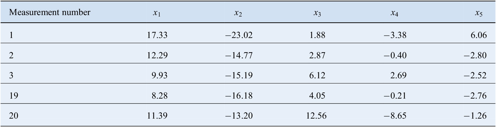
  $ {C}^1 $ from Equation (25) as the covariance, 20 points were randomly sampled. Twenty points were sampled because this asset belonged to the medium data category. An example of the condition data for this asset is shown in Table 2. The remaining 799 assets in the fleet were similarly simulated based on their model type, operating condition, and the category they belonged to. The complete training dataset can be found at: https://github.com/Dhada27/Hierarchical-Modelling-Asset-Fleets
Table 2. An example of condition data for a medium data category asset.
The proportion of assets belonging to the low data category were varied across a wide range from  $ 0.1 $ to $ 0.9 $. The remaining assets were evenly divided into medium and high data categories. For example, if $ 0.3 $ proportion of assets belonged to the low data category, then $ 0.35 $ proportion of assets belonged to high and medium data category each. Moreover, all clusters contained the same number of assets belonging to either of the three categories. Given this dataset, the goal for an anomaly detection algorithm was to model the assets’ normal operation by estimating the parameters of the underlying Gaussians. There was no indicator for the algorithm to know which cluster a given asset belonged to.
The testing dataset for each asset comprised of 1,500 points randomly sampled from the true underlying distribution, and 1,500 points sampled from the anomalous distribution. The deviations  $ l $ and $ L $ for the anomalous distributions were each varied while keeping the other constant, so that the sensitivity of the algorithms with respect to either parameters could be studied. Values of $ l $ were varied across $ \left\{\mathrm{0,5,10,20,50,100}\right\} $ while keeping $ L $ fixed at $ 1 $, and the values of $ L $ were varied across $ \left\{\mathrm{1,1.5,2,5,10}\right\} $ while keeping $ l $ fixed at $ 0 $.
4.2. Experimental design
The experiments involved comparing four learning scenarios as explained below.
1. Independent learning. In the first scenario, the assets were capable of learning from their own data only. This means that the only source of information for estimating the parameters of the underlying Gaussian was the given asset’s condition data only. The mean and covariance estimates in this scenario were evaluated according to the standard maximum likelihood estimation in Equations (23) and (24).
2. Learning from similar assets. In this scenario, the hierarchical model for the fleet was implemented. Clusters of similar assets were identified, and the parameters for the hierarchical model were estimated using the EM algorithm as explained in Section 3. The EM steps were iterated
$ 20 $ times, and the values of $ {\hat{\mu}}_i $ and $ {\hat{C}}_i $ after the 20th iteration were treated as the final estimates of hierarchical modeling. Twenty iterations were deemed sufficient for parameter estimation because the overall data log-likelihood did not increase any further. The value of $ K $, which are the number of clusters present in the fleet was set to its true value $ 4 $.3. Learning from all. The third scenario was similar to the one in Case 2 above, but with the difference being in this scenario the assets did not have a sense of identifying similar assets. This means that a given asset here learnt from all other assets in the fleet. To model this scenario, the same steps as those in Case 2 were followed, but the value of
$ K $ was set to 1. As a result, the entire fleet was treated as one cluster and the density function parameters of all assets shared a common underlying distribution.4. Only the low data assets learn from others. Finally, a combination of hierarchical and independent modeling was considered in the experiments. This scenario involved clustering and hierarchical modeling similar to the one in Case 2. But, while all 800 assets here participated in estimating hierarchical model parameters, only those assets belonging to the low data category used the final estimates for classifying the testing dataset. The medium and high data category assets used independent modeling to estimate their Gaussian parameters. Concretely, the final estimates for the assets belonging to the low data category were derived from the hierarchical model, whereas the final estimates for the assets belonging to the medium and high data category were derived from their independent models.


It was observed during the experiments that the accuracy of clustering using EM algorithm relied on the initialization of parameters, especially the  $ {\beta}_k $ and $ {\alpha}_k $ parameters. These parameters must be initialized such that the algorithm’s search space is wide enough and is not trapped in local optima during the early iterations. The approximate initializations of parameters to ensure a wider search space are mentioned in Section 3. However, even with the optimal initialization, the EM algorithm was unable to cluster the assets due to the wide range of means chosen.
This problem is highlighted in Figure 4, where a sample of 50 assets from each of the asset clusters was taken and the total 200 assets thus formed were clustered based on the available 5 and 6 data points only. The figures show both cases—where all assets had the same amount of data, and where the assets are divided into “low,” “medium,” and “high” data categories explained in Section 4.1.3. In the figures corresponding to the latter case, the assets belonging to the “low,” “medium,” and “high” data categories are represented in red, orange, and green colors, respectively. Also, the number of data points with assets belonging to the low data category were 5 and 6, and were constant for the remaining assets. In all figures, the assets with ids 1–50 belonged to the same cluster, 51–100 belonged to the next cluster, and so on. Therefore, these asset ids are expected to be clustered together, which was not the case for only initial five or six data points. The wrongly clustered assets are marked with the dotted red circle.

Figure 4. The figures represent the clustering done by the EM algorithm when the assets (low data category assets in c and d) have five and six data points only. The incorrectly clustered assets are marked with dotted red circle.
In the real world, this problem can be addressed by including certain categorical data along with the time series data. Categorical data can arise from the operational experience, such as asset’s environment, upkeep, operation, and so on. However, for the experimental results presented here, it was assured that the assets were correctly clustered in these cases. If it was found that an asset was wrongly clustered, it was manually reassigned to its correct cluster and the results evaluated again. The goal of the experiments is to demonstrate the advantage of hierarchical modeling over the conventional independent modeling on the effectiveness of collaborative learning between assets.
4.3. Performance evaluation
After the estimated model parameters are obtained, the operator must define a region in multidimensional space that encompasses the asset’s normal operations data. For the statistical classifiers, this region is often defined based on a critical value from the probability density function (PDF) values, such that any point having the PDF value less than the critical value will lie outside the region and be deemed anomalous. The critical value corresponds to an  $ \alpha $ significance level, which separates the most likely $ 100\ast \alpha \% $ points from the rest. In other words, the critical value separates $ 100\ast \alpha $ percentile data sampled from the rest.
For the case of multivariate Gaussians, this region is an ellipsoid, and determining its boundary corresponding to the required  $ \alpha $ level is numerically complex. This is because one cannot simply integrate the tails of the multivariate Gaussian and obtain the boundary corresponding to the required $ \alpha $ level. However, for a multivariate Gaussian with dimension $ d $, the squared Mahalanobis distance ( $ {D}_{md} $) of any point with respect to that Gaussian is standard Chi-squared with $ d $ degrees of freedom.Footnote 1 For a standard Chi-squared distribution, it is easy to obtain the PDF value separating the most likely $ 100\ast \alpha \% $ points from the rest. This fact can be used to determine if a given data point from the multivariate Gaussian falls within the $ \alpha $ level set by the operator or not.
For example, if the  $ \alpha $ level is set at 0.8, then the corresponding PDF value for a standard Chi-squared distribution can be obtained which would in fact be the critical value for the squared $ {D}_{md} $ of the points. Any point having the squared $ {D}_{md} $ greater than the critical value would be deemed anomalous. The p values corresponding to various $ \alpha $ levels for a standard five-dimensional Chi-squared distribution are shown in Table 3. These also act as the critical values for the squared $ {D}_{md} $ while generating the receiver operator characteristics (ROCs).
Table 3. Various  $ \alpha $ levels used while plotting the ROCs, and the corresponding $ {D}_{md} $ values for the current experiment.

Note. These correspond to a standard Chi-squared distribution with 5 degrees of freedom.
Abbreviation: ROC, receiver operator characteristic.
The squared Mahalanobis distance for any point  $ \mathbf{X} $ from a given Gaussian distribution with the estimated mean and covariance $ \hat{\boldsymbol{\mu}} $ and $ \hat{\mathbf{C}} $ is obtained as:
 $$ {D}_{md}^2={\left(\mathbf{X}-\hat{\boldsymbol{\mu}}\right)}^T{\hat{\mathbf{C}}}^{-1}\left(\mathbf{X}-\hat{\boldsymbol{\mu}}\right) $$
 Areas under the ROC curves were used as the performance metric for comparing hierarchical modeling and with the conventional independent modeling technique. This is a widely used evaluation metric for classification tasks and is often called the c-statistic. It provides an aggregate measure of classification performance across a wide range of  $ \alpha $ levels.
To plot an ROC, the  $ \alpha $ levels while classifying the testing dataset were varied across $ \left\{0.995,0.99,0.975,0.95,0.9,0.75,0.5,0.1,0.05,0.025,0.01,0.005\right\} $. An ROC curve was obtained for a single asset and its corresponding testing dataset by plotting the true positive rate (TPR) versus false positive rate (FPR) for each of the alpha levels mentioned above.
Consider a testing dataset with  $ {N}_P $ and $ {N}_N $ number of real positive and negative class data points, respectively. For the current use case, testing data points sampled from the true underlying distribution were labeled as “negative” class and those sampled from the anomalous distribution were labelled as “positive” class. If a classifier is tested using this dataset and the resulting output comprises of $ {N}_{TP} $ and $ {N}_{FP} $ true positives and false positives respectively, the TPR and FPR are evaluated according to:
 $$ TPR=\frac{N_{TP}}{N_P}\hskip2em FPR=\frac{N_{FP}}{N_N} $$
 The area under the ROC curve (AUC) was used as an indicator of the model’s performance for a given asset. From Equation (27), it can be observed that a higher AUC is characterized by a high TPR and a low FPR for some  $ \alpha $ level. A higher AUC means that the classifier is better capable of separating the positive and the negative class in the testing dataset. Therefore, higher the AUC, the better is the classifier. An example ROC for a medium data category asset and its corresponding AUC are shown in Figure 5. This ROC was evaluated for the parameters estimated based on hierarchical modeling.

Figure 5. An example receiver operator characteristic (ROC) for asset id 52 evaluated for testing dataset with  $ l $ and $ L $ equal to 0 and 10, respectively.
Such AUCs were evaluated for hierarchical modeling across the fleet and for each testing dataset, and were compared with those obtained using independent modeling.
4.4. Experimental results
4.4.1. Using the AUCs as the performance metric
For each of the four scenarios, the AUCs were evaluated for the assets in the fleet as explained in Section 4.3. Box plots for each low, medium, and high data category assets for the same testing dataset are shown in Figure 6, where “HL” stands for “hierarchical learning” where the final estimates are estimated based on the higher level model. Figure 6 also includes a combined box plot for all assets in the fleet and for the above described scenarios. These AUCs are presented as box plots. Results corresponding to a subset of test cases are presented here, and the same conclusions hold across all testing datasets. The corresponding testing dataset deviations for all figures are mentioned in their captions.

Figure 6. Shown here are the areas under the receiver operator characteristic curves (AUCs) measured for the experiment cases. The subset of assets across which the AUCs are measured are indicated in the corresponding captions. For all the above four plots, the deviation for anomalous data in the testing dataset was set at  $ 1 $ and $ 10 $ for $ l $ and $ L $, respectively.
As an interesting extension to the above described scenarios, the number of data points held by the low data category assets were gradually increased. The number of data points were increased from 5 till 21, so that classifier performances throughout the transition of the assets from low to the medium data category and beyond could be analyzed. While doing this, the number of points held by the medium and high data category assets were kept constant at their initial values. Figure 7 presents the effect of increasing data at the low data category assets, where  $ 0.2 $ proportion of assets initially belonged to the low data category. The corresponding testing datasets are mentioned in the subcaptions.

Figure 7. Box plots presenting the effect of gradually increasing data contained by the low data category assets. The captions denote the corresponding deviations in the testing dataset.
Furthermore, a learning scenario where all 800 assets held the same amount of data was also studied. This was done by simulating the fleet where all assets initially had five data points only, which were gradually increased to as high as 500 together across all assets. The classifier performances were studied throughout this transition. Figure 8 present the classifier performances when all assets contained the same amount of data. Other results obtained from the experiments described in Section 4.2 are presented in Appendix C.

Figure 8. Box plots presenting the effect of gradually increasing the data across all assets, when they all had same amount of data. The corresponding testing dataset deviations are denoted in the captions.
4.4.2. Using the Bhattacharyya distance as the performance metric
Apart from the performance evaluation metric presented in Section 4.3, the Bhattacharyya distance  $ \left({D}_B\right) $ was also used to compare the performances of hierarchical and independent asset models. $ {D}_B $ is a distance measure for two multivariate Gaussians, and is calculated according to Equation (28) for the Gaussians parameterized by $ \left({\boldsymbol{\mu}}_1,{\mathbf{C}}_1\right) $ and $ \left({\boldsymbol{\mu}}_2,{\mathbf{C}}_2\right) $ (Bhattacharyya, Reference Bhattacharyya1946). A lower value of $ {D}_B $ signifies that the given Gaussians are more similar. For the current application, $ {D}_B $ between the true and estimated Gaussians for all the assets were evaluated.
 $$ {D}_B=\frac{1}{8}{\left({\boldsymbol{\mu}}_1-{\boldsymbol{\mu}}_2\right)}^T{\left(\frac{{\mathbf{C}}_1+{\mathbf{C}}_2}{2}\right)}^{-1}\left({\boldsymbol{\mu}}_1-{\boldsymbol{\mu}}_2\right)+\frac{1}{2}\mathit{\ln}\left(\frac{ D et\left(\frac{{\mathbf{C}}_1+{\mathbf{C}}_2}{2}\right)}{\sqrt{ D et\left({\mathbf{C}}_1\right) Det\left({\mathbf{C}}_2\right)}}\right) $$
 The plots for the evaluated  $ {D}_B $ are presented in Figure 9. Figure 9a,b present $ {D}_B $ evaluated across all assets in the fleet, according to Equation (28), as the data points in the low data category assets were sequentially increased. Figure 9a corresponds to the case where the range of individual asset means lay within the range $ \left(-25,25\right) $ and $ \left(\mathrm{275,325}\right) $ for the two model types. Figure 9b corresponds to the narrower range of means $ \left(-5,5\right) $ and $ \left(\mathrm{295,305}\right) $ for the two model types. Covariances used to represent the asset operating conditions were the same for both figures and mentioned in Equation (25). The results presented in Figure 9 correspond to the same experimental setup as for Figure 7.

Figure 9. Box plots presenting the  $ {D}_B $ recorded across the assets belonging to the low data category. A lower value of $ {D}_B $ signifies that the given Gaussians are more similar.
5. Discussion
A better classifier for a given asset and a testing dataset is characterized by a higher AUC, and a lower  $ {D}_B $. However, while analyzing the performance of that classifier across the entire fleet, its consistency also plays a key role. An operator would prefer having a classifier showing consistent but slightly worse performance rather than an unreliable classifier which shows high AUC for some assets in the fleet but low for others. With this in mind, the following points are summarized from the results presented in Section 4.4:
1. It is inferred from Figures 6a–c that hierarchical modeling is beneficial for the assets belonging to the low data category only. For the assets belonging to the low data category, the classifiers obtained using hierarchical modeling show significantly higher AUCs and lower variances than the independent models learning from their own data. This is true especially until the proportion of low data assets in the fleet is less than or equal to
$ 0.6 $. The same fact is reiterated by Figures 7 and 9 where until a certain amount of data is accumulated by the asset, it is better for it to rely on hierarchical model estimates. While the threshold corresponds to 13 data points in Figures 7 and 9, the exact data requirement for the independent model depends on the intra-cluster asset similarities and variance in data, and therefore varies across applications.2. Figure 6 shows that learning from similar assets is more helpful than learning from all assets in the fleet. Learning from all resulted in higher variance in AUCs recorded across all assets, as shown in Figures 6a–c.

The aforementioned points are further highlighted by Figures C2 and C3 (in Appendix C) where the classifier performances for the low data category assets across various testing datasets are presented. In these figures again, the hierarchical model is seen to consistently outperform the independent model, and learning from similar assets shows much lesser variance than learning from all assets in the fleet.
3. Figure 8 shows that independent modeling is always the better option when all assets in the fleet contain same amount of data. This is true across the entire range from 5 data points until 500 and beyond. But, Figure 8 also represents that hierarchical modeling eventually converges and becomes similar to independent modeling when the assets keep generating data over time. This confirms our hypothesis that initially the hierarchical model estimates are weighted more toward the general fleet behavior. The trend seen in Figure 8 is an expected outcome because when all assets in the fleet have same amount of data, none of which are clearly indicative of the assets’ operating regime. Therefore, the general fleet behavior, which is a combined behavior observed across all assets, was not indicative of the correct operating regime as well.
4. It was observed that the performance of hierarchical model was affected by the choice of range of means mentioned in Section 4.1.3. A shorter range of means would signify that the assets were more similar to one another, resulting in an improved performance of the hierarchical model. This fact can be observed from the results from the same experiment with shorter ranges of means,
$ \left(-5,5\right) $ and $ \left(\mathrm{295,305}\right) $, presented in Appendix D and Figure 9 for both performance metrics.


6. Conclusion
This paper proposes the use of hierarchical model as a systematic method for the similar assets within a fleet to collaboratively learn from one another, and improve the performances of their statistical classifiers for anomaly detection. The asset condition monitoring data are modeled using multivariate Gaussians. But the hierarchical model, unlike conventional maximum likelihood estimation, involves higher level distributions from which the asset level Gaussian parameters are sampled. The higher level distributions are shared by the clusters of similar assets, where similarities arise by the virtue of the assets operating in similar conditions or being of the same model type. The higher level distributions for the covariances and the means of the asset level Gaussians are modeled using their conjugates, that is Inverse Wishart and Gaussian, respectively.
Comparing the Bhattacharyya distance for the two techniques, it can be concluded that hierarchical modeling significantly improves the performances of conventional classifiers in the early periods of asset operations. This is the period when sufficient training data are not available to estimate the Gaussian parameters using maximum likelihood methods. The higher level distributions are also representative of the general behavior of the asset fleet, that can be of interest to the operators who want an overall understanding the fleet performance.
7. Future Research Directions
This was the first use case of hierarchical modeling for anomaly detection in industrial asset operations, and interesting future research awaits.
1. The example implementation here was shown using a simulation fleet of assets. An interesting follow-up work would be to analyze how hierarchical modeling works for a real-world fleet of assets. Such analysis can include the extent of improvement in overall maintenance cost to the organization, and therefore, its business value can be justified. Moreover, the real world implementation would enable including the categorical data for clustering the assets and improve the accuracy of the EM algorithm. This is explained in Section 4.2.
2. Since anomaly detection algorithms are supposed to be implemented in real time, a follow up task is to extend the hierarchical model to an online version. The online version should classify each new data point as anomalous or not, and if the new data point is not anomalous it should be used to update the hierarchical model parameters.
3. An important conclusion from the experiments was that a low data category asset benefits the most from the hierarchical model. Moreover, that asset has nothing to contribute towards the general fleet knowledge. Therefore, it would be interesting to analyze how a hierarchical model would perform if only the medium and high data category assets were allowed to contribute to the higher level distributions, whereas the low data category assets only learn from them.
4. Finally, an important assumption while modeling the asset behaviors was that the mean of the Gaussian during an asset’s normal operation is constant. This might not always be the case. Sometimes, an asset’s operation could involve a sequence of tasks which could induce a cyclic nature to the Gaussian mean. Therefore, future research must focus on extending the current hierarchical model to account for natural deviations observed in the Gaussian mean throughout an asset’s operation.
Funding Statement
This research was funded by the EPSRC and BT Prosperity Partnership project: Next Generation Converged Digital Infrastructure, grant number EP/R004935/1. This research was also funded by Siemens Industrial Turbomachinery, Lincoln, UK LN5 7FD.
Competing Interests
The authors declare no competing interests.
Data Availability Statement
The data used to generate the results presented in this paper can be found in: https://github.com/Dhada27/Hierarchical-Modelling-Asset-Fleets
Author Contributions
Conceptualization, M.D., M.G., and A.K.P.; Methodology, M.G. and M.D.; Data curation, M.G., M.D., and A.K.P.; Data visualization, M.D. and A.K.P. Writing original draft, M.D. All authors approved the final submitted draft.
Acknowledgments
We are grateful for the discussions and feedbacks from Manuel Herrera, Marco Perez Hernandez, and Amit Kumar Jain from the Institute for Manufacturing, Cambridge CB3 0FS, UK.
A. Derivations of the E and M Steps
A.1. E-step
For the case of asset fleets, the E-step involves first evaluating the expectation of  $ \mathbf{z} $ w.r.t. distribution conditioned on $ \mathbf{X} $ for parameter values $ \boldsymbol{\theta} ={\boldsymbol{\theta}}^t $. Since $ {\mathbf{z}}_{i, k} $ is binary, $ \unicode{x1D53C}\left({\mathbf{z}}_{i, k}|{\left({\boldsymbol{\mu}}_i,{\mathbf{C}}_i\right)}^t,{\boldsymbol{\theta}}^t\right)= p\left({\mathbf{z}}_{i, k}=1|{\left({\boldsymbol{\mu}}_i,{\mathbf{C}}_i\right)}^t,{\boldsymbol{\theta}}^t\right)= p\left({\mathbf{z}}_{i, k}=1|{\left({\boldsymbol{\mu}}_i,{\mathbf{C}}_i\right)}^t,{\boldsymbol{\theta}}^t\right) $. Using Bayes’ rule
 $$ p\left({\mathbf{z}}_{i, k}=1|{\left({\boldsymbol{\mu}}_i,{\mathbf{C}}_i\right)}^t,{\boldsymbol{\theta}}^t\right)=\frac{p\left({\left({\boldsymbol{\mu}}_i,{\mathbf{C}}_i\right)}^t|{\mathbf{z}}_{i, k}=1,{\boldsymbol{\theta}}^t\right) p\left({\mathbf{z}}_{i, k}=1\right)}{\sum \limits_{k=1}^K p\left({\left({\boldsymbol{\mu}}_i,{\mathbf{C}}_i\right)}^t|{\mathbf{z}}_{i, k}=1,{\boldsymbol{\theta}}^t\right) p\left({\mathbf{z}}_{i, k}=1\right)} $$
from Equations (8) and (10) we know,
 $$ p\left({\mathbf{z}}_{i, k}=1|{\left({\boldsymbol{\mu}}_i,{\mathbf{C}}_i\right)}^t,{\boldsymbol{\theta}}^t\right)=\frac{\left( N\left({\boldsymbol{\mu}}_i|{\mathbf{m}}_k,{\beta}_k^{-1}{\mathbf{C}}_i\right) I W\left({\mathbf{C}}_i|{\boldsymbol{\Lambda}}_k,{\alpha}_k\right)\right)\left({\pi}_k\right)}{\sum \limits_{k=1}^K\left( N\left({\boldsymbol{\mu}}_i|{\mathbf{m}}_k,{\beta}_k^{-1}{\mathbf{C}}_i\right) I W\left({\mathbf{C}}_i|{\boldsymbol{\Lambda}}_k,{\alpha}_k\right)\right)\left({\pi}_k\right)} $$
 where all distribution parameters correspond to the values obtained at M-step of latest (tth) iteration. Let,  $ p\left({\mathbf{z}}_{i, k}=1|{\left({\boldsymbol{\mu}}_i,{\mathbf{C}}_i\right)}^t,{\boldsymbol{\theta}}^t\right)={\boldsymbol{\gamma}}_{i, k} $. Therefore, our function $ Q\left(\boldsymbol{\theta}, {\boldsymbol{\theta}}^t\right) $ can be deduced from Equation (14) by replacing $ {\mathbf{z}}_{i, k} $ with $ {\boldsymbol{\gamma}}_{i, k} $:
 $$ Q\left(\boldsymbol{\theta}, {\boldsymbol{\theta}}^t\right)=\sum \limits_{i=1}^I\sum \limits_{n=1}^{N_i}\log \left( N\left({\boldsymbol{\mu}}_i,{\mathbf{C}}_i\right)\right)+\sum \limits_{i=1}^I\sum \limits_{k=1}^K{\boldsymbol{\gamma}}_{i, k}\log \left({\pi}_k N\left({\boldsymbol{\mu}}_i|{\mathbf{m}}_k,{\beta}_k^{-1}{\mathbf{C}}_i\right) I W({\mathbf{C}}_i|{\boldsymbol{\Lambda}}_k,{\alpha}_k)\right) $$
 After substituting the symbolic representation with the corresponding distribution functions and parameters,  $ Q\left(\boldsymbol{\theta}, {\boldsymbol{\theta}}^t\right) $ (not including constant terms, because they would become zero after differentiation) becomes
 $$ {\displaystyle \begin{array}{l} Q\left(\boldsymbol{\theta}, {\boldsymbol{\theta}}^t\right)=\\ {}-\frac{1}{2}\sum \limits_i\sum \limits_n\mathit{\log}\mid {\mathbf{C}}_i\mid -\frac{1}{2}\sum \limits_i\sum \limits_n{\left({\mathbf{x}}_{i, n}-{\boldsymbol{\mu}}_i\right)}^T{\mathbf{C}}_i^{-1}\left({\mathbf{x}}_{i, n}-{\boldsymbol{\mu}}_i\right)-\\ {}\hskip1.5em \frac{1}{2}\sum \limits_i{\boldsymbol{\gamma}}_{i, k}\sum \limits_k\log \mid {\mathbf{C}}_i\mid +\frac{1}{2}\sum \limits_i{\boldsymbol{\gamma}}_{i, k}\sum \limits_k\log \left({\beta}_k\right)-\frac{1}{2}\sum \limits_i{\boldsymbol{\gamma}}_{i, k}\sum \limits_k{\beta}_k{\left({\boldsymbol{\mu}}_i-{\mathbf{m}}_k\right)}^T{\mathbf{C}}_i^{-1}\left({\boldsymbol{\mu}}_i-{\mathbf{m}}_k\right)+\\ {}\frac{1}{2}\sum \limits_i{\boldsymbol{\gamma}}_{i, k}\sum \limits_k{\alpha}_k\log \mid {\boldsymbol{\Lambda}}_k\mid -\frac{1}{2}\sum \limits_i{\boldsymbol{\gamma}}_{i, k}\sum \limits_k{\alpha}_k d\log (2)-\\ {}\hskip1.23em \sum \limits_i{\boldsymbol{\gamma}}_{i, k}\sum \limits_k\log \left({\Gamma}_d\left(\frac{\alpha_k}{2}\right)\right)-\frac{1}{2}\sum \limits_i{\boldsymbol{\gamma}}_{i, k}\sum \limits_k\left({\alpha}_k+ d+1\right)\log \mid {\mathbf{C}}_i\mid -\\ {}\hskip6.119996em \frac{1}{2}\sum \limits_i{\boldsymbol{\gamma}}_{i, k}\sum \limits_k Tr\left({\boldsymbol{\Lambda}}_k{\mathbf{C}}_i^{-1}\right)+\sum \limits_i{\boldsymbol{\gamma}}_{i, k}\sum \limits_k{\pi}_k\end{array}} $$
 The  $ {\boldsymbol{\gamma}}_{i, k} $ are not included in summations because they are supposed to be treated as constants in the M-step that follows.
A.2. M-step
In M-step,  $ {\boldsymbol{\theta}}^{t+1} $ values are obtained for following $ {\left( t+1\right)}^{th} $ E-step by maximizing the $ Q\left(\boldsymbol{\theta}, {\boldsymbol{\theta}}^t\right) $ function obtained in Equation (32) with respect to each of the $ \boldsymbol{\theta} $ parameters, and treating $ {\boldsymbol{\gamma}}_{i, k} $ as constants. Calculations for partial derivatives of $ Q\left(\boldsymbol{\theta}, {\boldsymbol{\theta}}^t\right) $ w.r.t. each parameter are shown below:
A.2.1. Evaluating $ {\hat{\boldsymbol{\mu}}}_i $

 $$ {\displaystyle \begin{array}{c}\frac{\mathit{\partial} Q\left(\boldsymbol{\theta}, {\boldsymbol{\theta}}^t\right)}{\mathit{\partial}{\boldsymbol{\mu}}_i}\Rightarrow \sum \limits_n{\mathbf{C}}_i^{-1}\left({\mathbf{x}}_{i, n}-{\boldsymbol{\mu}}_i\right)-\sum \limits_k{\beta}_k{\boldsymbol{\gamma}}_{i, k}{\mathbf{C}}_i^{-1}\left({\boldsymbol{\mu}}_i-{\mathbf{m}}_k\right)=0\\ {}\Rightarrow \sum \limits_n{\mathbf{x}}_{i, n}-{N}_i{\boldsymbol{\mu}}_i={\boldsymbol{\mu}}_i\sum \limits_k{\beta}_k{\boldsymbol{\gamma}}_{i, k}-\sum \limits_k{\beta}_k{\boldsymbol{\gamma}}_{i, k}{\mathbf{m}}_k\\ {}\Rightarrow {\hat{\boldsymbol{\mu}}}_i=\frac{1}{N_i+\sum \limits_{k=1}^K{\beta}_k{\boldsymbol{\gamma}}_{i, k}}\left[\sum \limits_{n=1}^{N_i}{\mathbf{x}}_{i, n}+\sum \limits_{k=1}^K{\beta}_k{\boldsymbol{\gamma}}_{i, k}{\mathbf{m}}_k\right]\end{array}} $$
A.2.2. Evaluating $ {\hat{\mathbf{m}}}_k $

 $$ {\displaystyle \begin{array}{c}\frac{\mathit{\partial} Q\left(\boldsymbol{\theta}, {\boldsymbol{\theta}}^t\right)}{\mathit{\partial}{\mathbf{m}}_k}\Rightarrow \sum \limits_i{\boldsymbol{\gamma}}_{i, k}{\beta}_k{\mathbf{C}}_i^{-1}\left({\boldsymbol{\mu}}_i-{\mathbf{m}}_k\right)=0\\ {}\Rightarrow {\beta}_k\sum \limits_i{\boldsymbol{\gamma}}_{i, k}{\mathbf{C}}_i^{-1}{\boldsymbol{\mu}}_i={\beta}_k\sum \limits_i{\boldsymbol{\gamma}}_{i, k}{\mathbf{C}}_i^{-1}{\mathbf{m}}_k\\ {}\Rightarrow \left[\sum \limits_i{\boldsymbol{\gamma}}_{i, k}{\mathbf{C}}_i^{-1}\right]{\mathbf{m}}_k=\left[\sum \limits_i{\boldsymbol{\gamma}}_{i, k}{\mathbf{C}}_i^{-1}{\boldsymbol{\mu}}_i\right]\\ {}\Rightarrow {\hat{\mathbf{m}}}_k={\left[\sum \limits_{i=1}^I{\boldsymbol{\gamma}}_{i, k}{\mathbf{C}}_i^{-1}\right]}^{-1}\left[\sum \limits_{i=1}^I{\boldsymbol{\gamma}}_{i, k}{\mathbf{C}}_i^{-1}{\boldsymbol{\mu}}_i\right]\end{array}} $$
A.2.3. Evaluating $ {\hat{\boldsymbol{\Lambda}}}_k $

 $$ {\displaystyle \begin{array}{c}\frac{\mathit{\partial} Q\left(\boldsymbol{\theta}, {\boldsymbol{\theta}}^t\right)}{\mathit{\partial}{\boldsymbol{\Lambda}}_k}\Rightarrow \frac{1}{2}\sum \limits_i{\boldsymbol{\gamma}}_{i, k}{\alpha}_k{\boldsymbol{\Lambda}}_k^{-1}-\frac{1}{2}\sum \limits_i{\boldsymbol{\gamma}}_{i, k}{\mathbf{C}}_i^{-1}=0\\ {}\Rightarrow {\boldsymbol{\Lambda}}_k^{-1}=\frac{\sum \limits_i{\boldsymbol{\gamma}}_{i, k}{\mathbf{C}}_i^{-1}}{\alpha_k\sum \limits_i{\boldsymbol{\gamma}}_{i, k}}\\ {}\Rightarrow {\hat{\boldsymbol{\Lambda}}}_k=\left[{\alpha}_k\sum \limits_{i=1}^I{\boldsymbol{\gamma}}_{i, k}\right]{\left[\sum \limits_{i=1}^I{\boldsymbol{\gamma}}_{i, k}{\mathbf{C}}_i^{-1}\right]}^{-1}\end{array}} $$
A.2.4. Evaluating $ {\hat{\beta}}_k $

 $$ {\displaystyle \begin{array}{c}\frac{\mathit{\partial} Q\left(\boldsymbol{\theta}, {\boldsymbol{\theta}}^t\right)}{\mathit{\partial}{\beta}_k}\Rightarrow \frac{d}{2}\sum \limits_i{\boldsymbol{\gamma}}_{i, k}\frac{1}{\beta_k}-\frac{1}{2}\sum \limits_i{\boldsymbol{\gamma}}_{i, k}{\left({\boldsymbol{\mu}}_i-{\mathbf{m}}_k\right)}^T{\mathbf{C}}_i^{-1}\left({\boldsymbol{\mu}}_i-{\mathbf{m}}_k\right)=0\\ {}\Rightarrow \frac{1}{{\hat{\beta}}_k}=\frac{\sum \limits_{i=1}^I{\boldsymbol{\gamma}}_{i, k}{\left({\boldsymbol{\mu}}_i-{\mathbf{m}}_k\right)}^T{\mathbf{C}}_i^{-1}\left({\boldsymbol{\mu}}_i-{\mathbf{m}}_k\right)}{d\sum \limits_{i=1}^I{\boldsymbol{\gamma}}_{i, k}}\end{array}} $$
A.2.5. Evaluating $ {\hat{\mathbf{C}}}_i $

 $$ {\displaystyle \begin{array}{ll}\frac{\mathit{\partial} Q\left(\boldsymbol{\theta}, {\boldsymbol{\theta}}^t\right)}{\mathit{\partial}{\mathbf{C}}_i}& \Rightarrow -\frac{N_i}{2}{\mathbf{C}}_i^{-1}+\frac{1}{2}{\mathbf{C}}_i^{-1}(\sum \limits_n\left({\mathbf{x}}_{i, n}-{\boldsymbol{\mu}}_i\right){\left({\mathbf{x}}_{i, n}-{\boldsymbol{\mu}}_i\right)}^T){\mathbf{C}}_i^{-1}\\ {}& -\frac{1}{2}{\mathbf{C}}_i^{-1}+\frac{1}{2}{\mathbf{C}}_i^{-1}(\sum \limits_k{\beta}_k{\boldsymbol{\gamma}}_{i, k}\left({\boldsymbol{\mu}}_i-{\mathbf{m}}_k\right){\left({\boldsymbol{\mu}}_i-{\mathbf{m}}_k\right)}^T){\mathbf{C}}_i^{-1}\\ {}& -\frac{1}{2}\sum \limits_k{\boldsymbol{\gamma}}_{i, k}\left({\alpha}_k+ d+1\right){\mathbf{C}}_i^{-1}+\frac{1}{2}\sum \limits_k{\boldsymbol{\gamma}}_{i, k}{\mathbf{C}}_i^{-1}{\Lambda}_k{\mathbf{C}}_i^{-1}=0\\ {}& \Rightarrow -\frac{N_i}{2}{\mathbf{C}}_i+\frac{1}{2}\sum \limits_n\left({\mathbf{x}}_{i, n}-{\boldsymbol{\mu}}_i\right){\left({\mathbf{x}}_{i, n}-{\boldsymbol{\mu}}_i\right)}^T-\frac{1}{2}{\mathbf{C}}_i\\ {}& +\frac{1}{2}\sum \limits_k{\beta}_k{\boldsymbol{\gamma}}_{i, k}\left({\boldsymbol{\mu}}_i-{\mathbf{m}}_k\right){\left({\boldsymbol{\mu}}_i-{\mathbf{m}}_k\right)}^T\\ {}& -\frac{1}{2}\sum \limits_k{\boldsymbol{\gamma}}_{i, k}\left({\alpha}_k+ d+1\right){\mathbf{C}}_i+\frac{1}{2}\sum \limits_k{\boldsymbol{\gamma}}_{i, k}{\Lambda}_k=0\\ {}& \Rightarrow ({N}_i+1+\sum \limits_k{\boldsymbol{\gamma}}_{i, k}{\alpha}_k+ d+1){\mathbf{C}}_i=\sum \limits_n\left({\mathbf{x}}_{i, n}-{\boldsymbol{\mu}}_i\right){\left({\mathbf{x}}_{i, n}-{\boldsymbol{\mu}}_i\right)}^T\\ {}& +\sum \limits_k{\beta}_k{\boldsymbol{\gamma}}_{i, k}\left({\boldsymbol{\mu}}_i-{\mathbf{m}}_k\right){\left({\boldsymbol{\mu}}_i-{\mathbf{m}}_k\right)}^T+\sum \limits_k{\boldsymbol{\gamma}}_{i, k}{\Lambda}_k\\ {}& \Rightarrow {\hat{\mathbf{C}}}_i=\\ {}& \frac{\sum \limits_{n=1}^{N_i}\left({\mathbf{x}}_{i, n}-{\boldsymbol{\mu}}_i\right){\left({\mathbf{x}}_{i, n}-{\boldsymbol{\mu}}_i\right)}^T+\sum \limits_{k=1}^K{\beta}_k{\boldsymbol{\gamma}}_{i, k}\left({\boldsymbol{\mu}}_i-{\mathbf{m}}_k\right){\left({\boldsymbol{\mu}}_i-{\mathbf{m}}_k\right)}^T+\sum \limits_{k=1}^K{\boldsymbol{\gamma}}_{i, k}{\Lambda}_k}{N_i+\sum \limits_{k=1}^K{\boldsymbol{\gamma}}_{i, k}{\alpha}_k+ d+2}\end{array}} $$
A.2.6. Evaluating $ {\hat{\alpha}}_k $

The below stated  $ f\left({\alpha}_k\right) $ must be maximised w.r.t. $ {\alpha}_k $:
 $$ {\displaystyle \begin{array}{l} f\left({\alpha}_k\right)=\frac{1}{2}{\alpha}_k\log \mid {\boldsymbol{\Lambda}}_k\mid \sum \limits_i{\boldsymbol{\gamma}}_{i k}-\frac{d}{2}\log (2){\alpha}_k\sum \limits_i{\boldsymbol{\gamma}}_{i k}-\\ {}\log \left({\Gamma}_d\left(\frac{\alpha_k}{2}\right)\right)\sum \limits_i{\boldsymbol{\gamma}}_{i k}-\frac{1}{2}\left({\alpha}_k+ d+1\right)\sum \limits_i{\boldsymbol{\gamma}}_{i k}\log \mid {\boldsymbol{C}}_i\mid \end{array}} $$
 But the presence of  $ \log \left({\Gamma}_d\left(\frac{\alpha_k}{2}\right)\right){\sum}_i{\boldsymbol{\gamma}}_{i k} $ term makes differentiation w.r.t. $ {\alpha}_k $ complex. Therefore, a nonlinear optimisation must be used for evaluating $ {\alpha}_k $ values at the M-step of every iteration. For the experiments discussed in this paper, the Broyden–Fletcher–Goldfarb–Shanno (BFGS) algorithm was used to minimize $ - f\left({\alpha}_k\right) $, with limits set as $ {\alpha}_k\hskip0.30em \in \hskip0.30em \left( d, d+20\right) $.
A.2.7. Evaluating $ {\hat{\boldsymbol{\pi}}}_k $

Evaluating  $ {\hat{\boldsymbol{\pi}}}_k $ is a constrained optimisation problem, because $ {\pi}_k $ also have to satisfy an additional condition of $ {\sum}_k{\pi}_k=1 $. Therefore, we need to maximize $ \left[ Q\left(\boldsymbol{\theta}, {\boldsymbol{\theta}}^t\right)+\eta \left({\sum}_k{\pi}_k-1\right)\right] $ w.r.t. $ {\pi}_k $, where $ \eta $ is the Lagrange multiplier. From Equation (32), we have
 $$ {\displaystyle \begin{array}{c}\frac{\mathit{\partial}\left[ Q\left(\boldsymbol{\theta}, {\boldsymbol{\theta}}^t\right)+\eta (\sum \limits_k{\pi}_k-1)\right]}{\mathit{\partial}{\pi}_k}\Rightarrow \frac{\sum \limits_i{\boldsymbol{\gamma}}_{i, k}}{\pi_k}+\eta =0\\ {}\Rightarrow {\pi}_k=\frac{-\sum \limits_i{\boldsymbol{\gamma}}_{i, k}}{\eta}\end{array}} $$
 But, since  $ {\sum}_k{\pi}_k=1 $; $ \eta =\eta \left({\sum}_k{\pi}_k\right)=-{\sum}_i{\sum}_k{\boldsymbol{\gamma}}_{i, k} $ (from above) $ =- I $ (by definition, because these are also the expectations of $ {\mathbf{z}}_{i, k} $) where $ I $ are total assets in the fleet. Substituting value of $ \eta $ in above equation, we get
 $$ {\hat{\boldsymbol{\pi}}}_k=\frac{\sum \limits_{i=1}^I{\boldsymbol{\gamma}}_{i, k}}{I} $$
B. Proof for the Chi-squared Nature of the Squared Mahalanobis Distance
Proof for the standard Chi-squared nature of the squared Mahalanobis distances ( $ {D}_{md}^2 $) of points with respect to a $ d $ dimensional multivariate Gaussian is presented here. This proof is provided for the sake of completeness, where basic knowledge of linear algebra is assumed. The reader is advised to refer (Thill, Reference Thill2017) for the complete derivation, and also the empirical proof.
For any given point  $ X $ in space, its squared Mahalanobis distance ( $ {D}_{md}^2 $) with respect to a multivariate Gaussian with mean $ \mu $ and covariance $ \boldsymbol{\Sigma} $ is evaluated as (assuming orthonormal eigenvectors):
 $$ {D}_{md}^2={\left( X-\boldsymbol{\mu} \right)}^T{\boldsymbol{\Sigma}}^{-1}\left( X-\boldsymbol{\mu} \right) $$
 Upon performing he eigenvalue decomposition of  $ {\boldsymbol{\Sigma}}^{-1} $, one obtains
 $$ {\boldsymbol{\Sigma}}^{-1}= U{\Lambda}^{-1}{U}^{-1}= U\Lambda {U}^T=\sum \limits_{k=1}^d{\lambda}_k^{-1}{u}_k{u}_k^T $$
where  $ {u}_k $ is the $ {k}^{th} $ eigenvector of the corresponding eigenvalue $ {\lambda}_k $.
Therefore,
 $$ {D}_{md}={\left( X-\boldsymbol{\mu} \right)}^T{\boldsymbol{\Sigma}}^{-1}\left( X-\boldsymbol{\mu} \right) $$
 $$ ={\left( X-\boldsymbol{\mu} \right)}^T\left(\sum \limits_{k=1}^d{\lambda}_k^{-1}{u}_k{u}_k^T\right)\left( X-\boldsymbol{\mu} \right) $$
 $$ =\sum \limits_{k=1}^d{\lambda}_k^{-1}{\left( X-\boldsymbol{\mu} \right)}^T{u}_k{u}_k^T\left( X-\boldsymbol{\mu} \right) $$
 $$ =\sum \limits_{k=1}^d{\lambda}_k^{-1}{\left[{\mu}_k^T\left( X-\boldsymbol{\mu} \right)\right]}^2 $$
 $$ =\sum \limits_{k=1}^d\left[{\lambda}_k^{\frac{-1}{2}}{\mu}_k^T\left( X-\boldsymbol{\mu} \right)\right] $$
 $$ =\sum \limits_{k=1}^d{Y}_k^2 $$
where  $ {Y}_k $ is a new random variable based on affine linear transformation of the random vector $ X $.
We know that a random variable  $ Z=\left( X-\boldsymbol{\mu} \right) $ can be expressed as $ Z\sim N\left(0,\boldsymbol{\Sigma} \right) $. Similarly, the random variable $ {Y}_k $ introduced in Equations (38) is of the form $ {Y}_k={\lambda}_k^{\frac{-1}{2}}{\mu}_k^T Z $. It can therefore be expressed as $ {Y}_k\sim N\left(0,{\boldsymbol{\Sigma}}_k^2\right) $ where
 $$ {\displaystyle \begin{array}{c}{\boldsymbol{\Sigma}}_k^2={\lambda}_k^{\frac{-1}{2}}{u}_k^T\boldsymbol{\Sigma} {\lambda}_k^{\frac{-1}{2}}{u}_k\\ {}={\lambda}_k^{-1}{u}_k^T\boldsymbol{\Sigma} {\mu}_k\end{array}} $$
 Upon substituting  $ \boldsymbol{\Sigma} ={\sum}_{j=1}^d{\lambda}_j{u}_j{u}_j^T $,
 $$ {\displaystyle \begin{array}{c}{\boldsymbol{\Sigma}}_k^2={\lambda}_k^{-1}{u}_k^T\boldsymbol{\Sigma} {\mu}_k\\ {}={\lambda}_k^{-1}{u}_k^T\left(\sum \limits_{j=1}^d{\lambda}_j{u}_j{u}_j^T\right){\boldsymbol{\mu}}_k\\ {}=\sum \limits_{j=1}^d{\lambda}_k^{-1}{u}_k^T{\lambda}_j{u}_j{u}_j^T{u}_k\\ {}=\sum \limits_{j=1}^d{\lambda}_k^{-1}{\lambda}_j{u}_k^T{u}_j{u}_j^T{u}_k\end{array}} $$
 Since all eigenvectors  $ {u}_i $ are pairwise orthonormal, the dotted products $ {u}_k^T{u}_j $ and $ {u}_j^T{u}_k $ will be zero for $ j\ne k $. Only for the case $ j= k $ we get
 $$ {\displaystyle \begin{array}{c}{\boldsymbol{\Sigma}}_k^2={\lambda}_k^{-1}{\lambda}_k{u}_k^T{u}_k{u}_k^T{u}_k\\ {}={\lambda}_k^{-1}{\lambda}_k{\left\Vert {u}_k\right\Vert}^2{\left\Vert {u}_k\right\Vert}^2\\ {}=1\end{array}} $$
The last step follows because the norm  $ \Vert {u}_k\Vert $ of an orthonormal eigenvector is equal to 1. The squared $ {D}_{md} $ can thus be expressed as $ {D}_{md}^2={\sum}_{k=1}^d{Y}_k^2 $ where $ {Y}_k\sim N\left(0,1\right) $. This is also the exact definition of a standard chi-squared distribution with $ d $ degrees of freedom, that is the sum of the squared of $ d $ random variables which are standard normally distributed. Therefore, the squared $ {D}_{md} $ is Chi-squared with $ d $ degrees of freedom and can therefore be used to obtain a critical value for anomaly detection.
C. Continued Result Figures from the Experiments, Demonstrating the Benefit of Hierarchical Modeling for the Low Data Category Assets

Figure C1. Box plots presenting the effect of gradually increasing data contained by the low data category assets. The captions denote the corresponding deviations in the testing dataset.

Figure C2. Box plots presenting AUCs recorded across the assets belonging to the low data category. The corresponding testing dataset deviations are denoted in the captions.

Figure C3. Box plots presenting AUCs recorded across the assets belonging to the low data category. The corresponding testing dataset deviations are denoted in the captions.
D. Results from the Experiment Conducted for a Shorter Range of Asset Means
Figure D1 shows the comparison of performances of the hierarchical model and independent learning for the clusters with a narrow range of means representing the asset model types. The asset clusters comprised of means ranging within  $ \left(-5,5\right) $ for one model type and $ \left(\mathrm{295,305}\right) $ for the other. The covariance matrices used to generate data were the same as the ones shown in Equations (25). A slight improvement in performance of the hierarchical model can be observed, due to the fact that the assets in a cluster here are more similar to one another. Figure D1 is evaluated in the same manner as Figure C1, but for the training and testing datasets corresponding to a narrower range of means.

Figure D1. Box plots presenting area under the receiver operator characteristic curves (AUCs) recorded across the assets belonging to the low data category, but for a narrower range of means.


 Open access
Comments
No Comments have been published for this article.