


Introduction
Mapping geographical ranges and identifying the environmental requirements of threatened species are fundamental research areas in conservation biology (Riddle et al. Reference Riddle, Ladle, Lourie, Whittaker, Ladle and Whittaker2011). Defining species’ spatial and ecological range limits is essential to assess the various threats facing many taxa in rapidly changing environments (Ladle and Whittaker Reference Ladle and Whittaker2011), and to formulate viable conservation plans for species survival (Margules and Pressey Reference Margules and Pressey2000, Sutton et al. Reference Sutton, Anderson, Franco, McClure, Miranda, Vargas, Vargas González and Puschendorf2021a). However, significant knowledge gaps still exist regarding the full area of distribution and environmental attributes of where individual species occur, commonly termed the “Wallacean Shortfall” (Lomolino Reference Lomolino, Lomolino and Heaney2004). The Wallacean Shortfall contributes to a second knowledge deficit where, if the current range of a species is unknown or not fully described, it is not possible to determine whether and when a species is in decline or possibly gone extinct. Thus, the environmental factors that limit the distribution and abundance of many threatened species are still poorly understood (Marcer et al. Reference Marcer, Sáez, Molowny-Horas, Pons and Pino2013).
A current biogeographical paradigm is that climate plays a central role in determining species distributions at broad scales (Pearson and Dawson Reference Pearson and Dawson2003). However, recent work has demonstrated that biotic interactions (Aragón et al. Reference Aragón, Carrascal and Palomino2018, Sutton et al. Reference Sutton, Anderson, Franco, Gomes, McClure, Miranda, Vargas, Vargas González, de and Puschendorf2023a), landcover (Tuanmu and Jetz Reference Tuanmu and Jetz2014, Reference Tuanmu and Jetz2015), and topography (Meineri and Hylander Reference Meineri and Hylander2017) are also important in setting range limits for many taxa. Species Distribution Models (SDMs) are a group of geospatial statistical methods that assess species–habitat associations and predict distribution based on correlating environmental covariates with species occurrences (Matthiopoulos et al. Reference Matthiopoulos, Fieberg and Aarts2020). SDMs can be effective in estimating potential range limits and ecological associations using satellite remote-sensing data coupled with occurrences from unstructured surveys and community science projects (Bradter et al. Reference Bradter, Mair, Jönsson, Knape, Singer and Snäll2018); this includes data for threatened species distributed across remote, hard to survey areas (Sutton et al. Reference Sutton, Anderson, Franco, McClure, Miranda, Vargas, Vargas González and Puschendorf2021b, Reference Sutton, Ibañez, Salvador, Taraya, Opiso, Senarillos and McClure2023b).
The endemic Madagascar Serpent-eagle Eutriorchis astur is a cryptic, medium-sized raptor with a restricted distribution across tropical forests in eastern Madagascar (BirdLife International 2016). The species is one of the rarest raptors globally and is currently classified as “Endangered” on the International Union for Conservation of Nature (IUCN) Red List (BirdLife International 2016). This forest-dependent raptor was once considered extinct but was rediscovered three decades ago by Peregrine Fund biologists (Thorstrom et al. Reference Thorstrom, Watson, Damary, Toto, Baba and Baba1995). Madagascar Serpent-eagles generally prefer uninterrupted expanses of lowland and mid-altitude tropical forest, with habitat loss and fragmentation the primary threats to the species future persistence (Thorstrom and Rene de Roland Reference Thorstrom and Rene de Roland2000). Despite being termed a serpent-eagle, snakes comprise only a small proportion of Madagascar Serpent-eagle prey, with chameleons and geckos accounting for >80% of diet (Thorstrom and Rene de Roland Reference Thorstrom and Rene de Roland2000). Recent research suggests the Madagascar Serpent-eagle may be vulnerable to both climate change (Andriamasimanana and Cameron Reference Andriamasimanana and Cameron2013) and increasing forest fragmentation (Benjara et al. Reference Benjara, Rene de Roland, Rakotondratsima and Thorstrom2021).
From surveys using playback techniques (Thorstrom and Rene de Roland Reference Thorstrom and Rene de Roland2000), the known range of the Madagascar Serpent-eagle is now thought to be considerably larger than previously estimated and it may not be as rare as once thought (BirdLife International 2016). However, a recent global assessment of human threats to raptor distributions identified the Madagascar Serpent-eagle as a priority species for conservation intervention to prevent likely extinction due to having >90% of its range impacted by forest loss (O’Bryan et al. Reference O’Bryan, Allan, Suarez-Castro, Delsen, Buij, McClure, Rehbein, Virani, McCabe, Tyrrell and Negret2022). Moreover, the environmental determinants of Madagascar Serpent-eagle distribution and abundance are still largely unknown. The global population is still very small, estimated between 250 and 999 mature individuals, and is likely to be decreasing (BirdLife International 2016). Spatial modelling can therefore help to determine the key ecological requirements of the Madagascar Serpent-eagle and update range metrics and population size estimates, both currently identified as priority areas of research (Thorstrom et al. Reference Thorstrom, Watson, Damary, Toto, Baba and Baba1995, Thorstrom and Rene de Roland Reference Thorstrom and Rene de Roland2000, BirdLife International 2016). Further, predicting the distributional potential for the Madagascar Serpent-eagle would enable specific hypotheses to be developed and tested on the processes limiting its distribution. This includes directing current field sampling protocols to identify potential areas of occupation (sensu Peterson and Anamza Reference Peterson and Anamza2015).
Improving the predictive power of spatial models by incorporating biotic, landcover, and topographical predictors derived from satellite remote sensing would also lead to higher certainty on where to designate new protected areas, strengthening the existing protected area network (Elith and Leathwick Reference Elith, Leathwick, Moilanen, Wilson and Possingham2009). Applying this knowledge to current conservation management can then direct designation of protected areas in line with suitable environmental areas (Sutton et al. Reference Sutton, Ibañez, Salvador, Taraya, Opiso, Senarillos and McClure2023b). Given this background, our aims were to apply spatial predictive modelling to estimate distribution and identify ecological range limits for the Madagascar Serpent-eagle. Our key objective was to use this information to inform current spatial conservation planning and estimate a potential population size. Here, we set out baseline estimates for: (1) the current distribution of the Madagascar Serpent-eagle based on remote-sensing habitat covariates; (2) identification of range-wide species–habitat associations; (3) updated IUCN range metrics and a population size estimate. From these baselines we then calculated protected area coverage, and conducted a gap analysis to identify priority designations for new protected areas.
Methods
Study extent and species locations
We defined the species’ accessible area (Barve et al. Reference Barve, Barve, Jiménez-Valverde, Lira-Noriega, Maher, Peterson, Soberón and Villalobos2011) as the ecoregions corresponding to both Madagascar lowland and subhumid tropical forest extracted from the World Wildlife Fund terrestrial ecoregions shapefile (Olson et al. Reference Olson, Dinerstein, Wikramanayake, Burgess, Powell, Underwood, D’amico, Itoua, Strand, Morrison and Loucks2001) (Figure 1). We masked out the remaining ecoregions in the far north, east, and south of Madagascar because the Madagascar Serpent-eagle is a habitat specialist of moist tropical forest (Thorstrom and Rene de Roland Reference Thorstrom and Rene de Roland2000, Benjara et al. Reference Benjara, Rene de Roland, Rakotondratsima and Thorstrom2021), and has not been recorded outside these ecoregions. We compiled a database of 33 Madagascar Serpent-eagle point localities from the Global Raptor Impact Network (GRIN), a global population monitoring information system for all raptors (McClure et al. Reference McClure, Anderson, Buij, Dunn, Henderson, McCabe and Tavares2021). For the Madagascar Serpent-eagle, GRIN consists of locations from unstructured surveys which only recorded presence (n = 24), a literature search (n = 4; Sheldon and Duckworth Reference Sheldon and Duckworth1990, Raxworthy and Colston Reference Raxworthy and Colston1992, Hawkins et al. Reference Hawkins, Thiollay, Goodman and Goodman1998, Karpanty and Grella Reference Karpanty and Grella2001), and community science data from the Global Biodiversity Information Facility (n = 5; GBIF 2020) (see Supplementary Materials).

Figure 1. Current IUCN range map for the Madagascar Serpent-eagle with our model accessible area derived from the tropical moist forest ecoregions (light grey) and IUCN range map (khaki). The dark grey polygon defines the national boundary of Madagascar not within the species accessible area.
Habitat covariate models
We considered eight potential habitat covariates a priori related empirically to known Madagascar Serpent-eagle habitat associations (Thorstrom and Rene de Roland Reference Thorstrom and Rene de Roland2000, Benjara et al. Reference Benjara, Rene de Roland, Rakotondratsima and Thorstrom2021). These were derived from satellite remote-sensing products representing climate, landcover, topography, and vegetation at a spatial resolution of 30 arc-seconds (~1 km resolution, Table 1). We downloaded raster layers from the EarthEnv (www.earthenv.org), ENVIREM (Title and Bemmels Reference Title and Bemmels2018), and Dynamic Habitat Indices (Radeloff Reference Radeloff, Dubinin, Coops, Allen, Brooks, Clayton, Costa, Graham, Helmers, Ives and Kolesov2019) repositories, which were then cropped and masked to a delimited polygon representing the species accessible area (Figure 1). The Climatic Moisture Index is a scaled measure (-1≤ Climatic Moisture Index ≤1) of the ratio of annual precipitation and annual evapotranspiration (Willmott and Feddema Reference Willmott and Feddema1992), used here as a proxy for moist tropical forest coverage. Evergreen Forest is a measure of percentage landcover here representing broadleaf tropical evergreen forest derived from consensus products integrating GlobCover (v2.2), MODIS landcover product (v051), GLC2000 (v1.1), and DISCover (v2) from the years 1992–2006. Full details on methodology and image processing for evergreen forest can be found in Tuanmu and Jetz (Reference Tuanmu and Jetz2014).
Table 1. Habitat covariates selected a priori and considered as potential covariates used in all spatial analyses for the Madagascar Serpent-eagle. FPAR = Fraction of absorbed Photosynthetically Active Radiation; NDVI = Normalised Difference Vegetation Index.
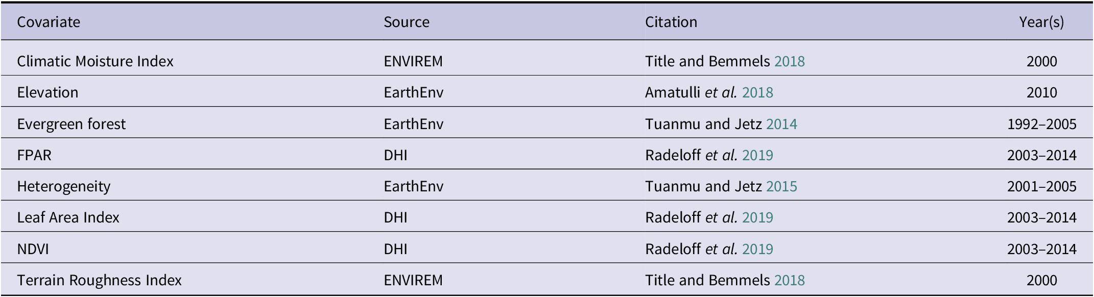
Heterogeneity is a biophysical texture measure closely related to vegetation structure, composition, and diversity (i.e. species richness) derived from textural features of the Enhanced Vegetation Index between adjacent pixels; sourced from the Moderate Resolution Imaging Spectroradiometer (MODIS) (https://modis.gsfc.nasa.gov/). We inverted the raster cell values in the original EarthEnv variable “Homogeneity” (Tuanmu and Jetz Reference Tuanmu and Jetz2015) to represent the spatial variability and arrangement of vegetation species richness on a continuous scale which varies between zero (minimum heterogeneity, low species richness) and one (maximum heterogeneity, high species richness). Elevation was derived from a digital elevation model product from the 250m Global Multi-Resolution Terrain Elevation Data 2010 (Danielson and Gesch Reference Danielson and Gesch2011). The Terrain Roughness Index is a measure of variation in topography around a central pixel, with lower values indicating flat terrain and higher values indicating larger differences in elevation of neighbouring pixels (Wilson et al. Reference Wilson, O’Connell, Brown, Guinan and Grehan2007).
Last, we used three biophysical vegetation layers based on averaged 8- and 16-day MODIS vegetation products, used here as composite Dynamic Habitat Index products (Radeloff et al. Reference Radeloff, Dubinin, Coops, Allen, Brooks, Clayton, Costa, Graham, Helmers, Ives and Kolesov2019). We used the single composite phenology curve product for each Dynamic Habitat Index vegetation layer, summarising three measures of vegetation productivity between 2003 and 2014: annual cumulative, minimum throughout the year, and seasonality as the annual coefficient of variation. The Normalised Difference Vegetation Index (NDVI) provides a measure of photosynthetic activity linked to species richness and productivity (Huete et al. Reference Huete, Didan, Miura, Rodriguez, Gao and Ferreira2002). However, NDVI can saturate in dense vegetation and highly productive areas (such as moist tropical forests) and cannot distinguish differences in productivity in these areas (Huete et al. Reference Huete, Didan, Miura, Rodriguez, Gao and Ferreira2002). Therefore, we used two further measures that directly assess productivity, providing a more accurate proxy for vegetation coverage: Leaf Area Index and Fraction of absorbed Photosynthetically Active Radiation (FPAR).
Both the Leaf Area Index and FPAR incorporate landcover in their calculation and use reflectance values from up to seven MODIS bands, compared with the two or three bands for NDVI and Enhanced Vegetation Index, respectively (Hobi et al. Reference Hobi, Dubinin, Graham, Coops, Clayton, Pidgeon and Radeloff2017). The Leaf Area Index is a measure of the amount of foliage within the plant canopy and a key driver of primary productivity (Asner et al. Reference Asner, Scurlock and Hicke2003). FPAR is a measure of productivity inferred from available photosynthetic activity driven by solar radiation (Myneni et al. Reference Myneni, Hoffman, Knyazikhin, Privette, Glassy, Tian, Wang, Song, Zhang, Smith and Lotsch2002), characterising the energy absorption of the vegetation canopy. The Leaf Area Index and FPAR are closely related measures, with the Leaf Area Index recommended for high productivity areas and FPAR for lower productivity areas (Radeloff et al. Reference Radeloff, Dubinin, Coops, Allen, Brooks, Clayton, Costa, Graham, Helmers, Ives and Kolesov2019). Combined, we used each Dynamic Habitat Index as proxies for food availability, assuming summarising vegetation productivity annually over the 11-year period captures seasonal variations in prey species habitat, and thus the availability of prey species that Madagascar Serpent-eagles would use as food (Hobi et al. Reference Hobi, Dubinin, Graham, Coops, Clayton, Pidgeon and Radeloff2017).
We selected covariates to use in our final model based on an information theoretical approach using Akaike’s Information Criterion (AIC) (Akaike Reference Akaike1974) corrected for small sample sizes (Hurvich and Tsai Reference Hurvich and Tsai1989) in the R package AICcmodavg (Mazerolle Reference Mazerolle2020). We fitted six candidate models using logistic regression with a binomial error term and logit link function using Generalised Linear Models (GLMs) in the R package stats (R Core Team 2018). We fitted all candidate models to derive maximum likelihood estimates on model parameters significantly different from zero, with no interaction terms. We standardised all predictors with a mean of zero and standard deviation (SD) of one. As the occurrence data correspond to a presence-only dataset, we randomly sampled background availability using 10,000 pseudo-absence points suitable for regression-based modelling (Barbet-Massin et al. Reference Barbet‐Massin, Jiguet, Albert and Thuiller2012). We assigned equal weights to both presence and background points allowing consistent sampling across the model calibration area. We did this to avoid saturating the models with excessive absence weighting, which makes presence trends difficult to detect (Elith and Leathwick Reference Elith and Leathwick2007).
First, we fitted model 1 with all eight covariates representing climate, landcover, topography, and vegetation, model 2 with only landcover, topography, and vegetation variables, and model 3 with landcover and vegetation plus elevation, but without Terrain Roughness Index. We fitted model 4 only considering landcover and vegetation variables, and finally, models 5 and 6 were fitted with landcover and vegetation both with and without NDVI and FPAR. We did not include an intercept-only model because its ΔAICc score was not competitive (ΔAICc = 20.75). We fitted linear terms to all model covariates except for the Climatic Moisture Index and Terrain Roughness Index, which were fitted with quadratic terms because we expected values of both covariates to be highest at intermediate values and decrease at lower and higher values. We considered all candidate models with an ΔAICc <2 as having strong support (Burnham and Anderson Reference Burnham and Anderson2004), and we selected the best supported model using the lowest ΔAICc and highest AICc weighting. We tested all covariates for multicollinearity directly at the Madagascar Serpent-eagle occurrences prior to model ranking and then as a final check on our best supported model covariates considering Variance Inflation Factors <2 (Dormann et al. Reference Dormann, Elith, Bacher, Buchmann, Carl, Carré, Marquéz, Gruber, Lafourcade, Leitão and Münkemüller2013).
SDMs
After identifying the most parsimonious model covariates using binomial GLMs, we fitted candidate SDMs, further tuning model parameters using penalised elastic net logistic regression in the R package maxnet (Phillips et al. Reference Phillips, Anderson, Dudík, Schapire and Blair2017). Penalising regression model coefficients reduces model variance, resulting in a regression model that generalises better than standard logistic regression (Valavi et al. Reference Valavi, Guillera‐Arroita, Lahoz‐Monfort and Elith2021). Penalised logistic regression imposes a regularisation penalty to the model coefficients reducing model complexity by shrinking the covariates that contribute the least to model prediction (Gastón and García-Viñas Reference Gastón and García-Viñas2011, Fithian and Hastie Reference Fithian and Hastie2013). An elastic net is used to perform automatic variable selection and continuous shrinkage simultaneously (via the glmnet package) (Friedman et al. Reference Friedman, Hastie and Tibshirani2010), retaining all covariates that contribute less by shrinking coefficients to either exactly zero or close to zero. We fitted SDMs via maximum penalised likelihood estimation using a complementary log-log (cloglog) link function as a continuous index of environmental suitability, with 0 = low suitability and 1 = high suitability. We parametrised the penalised logistic regression model using infinite weighting (presence weights = 1, background = 100) equivalent to an inhomogeneous Poisson process because this is the most effective method to model presence-background data as used here (Warton and Shepherd Reference Warton and Shepherd2010).
We used a random sample of 10,000 background points as pseudo-absences recommended for regression-based modelling (Barbet-Massin et al. Reference Barbet‐Massin, Jiguet, Albert and Thuiller2012), and to sufficiently sample the background calibration environment (Guevara et al. Reference Guevara, Gerstner, Kass and Anderson2018). We based optimal-model selection on AIC (Akaike Reference Akaike1974), corrected for small sample sizes (AICc) (Hurvich and Tsai Reference Hurvich and Tsai1989), to determine the most parsimonious model from two model parameters: regularisation beta multiplier (β; level of coefficient penalty) and feature classes (response functions; Warren and Seifert Reference Warren and Seifert2011). We considered 27 candidate models of varying complexity by conducting a grid search using a range of regularisation multipliers from 1 to 5 in 0.5 increments, and three feature classes (response functions: linear, quadratic, and hinge) in all possible combinations using the “jackknife” method of k-fold cross validation within the R package ENMeval (Muscarella et al. Reference Muscarella, Galante, Soley‐Guardia, Boria, Kass, Uriarte and Anderson2014).
The n –1 jackknife cross-validation approach is specifically used to test predictions using small occurrence datasets where the number of k folds is equal to the number of occurrences (n). All records but one are used in each model iteration, rather than losing valuable records via data splitting, with the single withheld record used once for testing (Gerstner et al. Reference Gerstner, Kass, Kays, Helgen and Anderson2018). From each withheld test record, n models are calibrated and evaluated at each iteration across all n models (Shcheglovitova and Anderson Reference Shcheglovitova and Anderson2013). We considered all models with an ΔAICc <2 as having strong support (Burnham and Anderson Reference Burnham and Anderson2004), with the model that had the lowest ΔAICc that used all three feature classes selected as the best supported model. We assessed variable performance using response functions and parameter estimates within the best supported calibration SDM. We used the Continuous Boyce Index (Hirzel et al. Reference Hirzel, Le Lay, Helfer, Randin and Guisan2006) as a measure of how predictions differ from a random distribution of observed presences (Boyce et al. Reference Boyce, Vernier, Nielsen and Schmiegelow2002). Last, we tested the optimal model against random expectations using partial Receiver Operating Characteristic ratios (pROC), which estimate model performance by giving precedence to omission errors over commission errors (Peterson et al. Reference Peterson, Papeş and Soberón2008) (see Supplementary Materials).
Range metrics and population size estimation
We followed the spatial modelling framework of Sutton et al. (Reference Sutton, Ibañez, Salvador, Taraya, Opiso, Senarillos and McClure2023b) and converted the final range-wide continuous prediction into a binary threshold prediction which we term model area of habitat (AOH), to be distinct from the standard IUCN AOH methodology (Brooks et al. Reference Brooks, Pimm, Akçakaya, Buchanan, Butchart, Foden, Hilton-Taylor, Hoffmann, Jenkins, Joppa and Li2019). To calculate model AOH in suitable pixels we reclassified the continuous prediction to a binary threshold using all pixel values equal to or greater than maximising the sum of sensitivity and specificity (maxTSS) from the continuous model prediction. We used maxTSS because it is the most appropriate threshold for SDM conservation applications using presence-only data (Liu et al. Reference Liu, White and Newell2013). We calculated two further IUCN range metrics from our model AOH binary prediction in the R package redlistr (Lee et al. Reference Lee, Keith, Nicholson and Murray2019). To do this we first converted the model AOH raster to a polygon using an eight-neighbour patch rule and applied a smoothing function using the Chaikin algorithm (Chaikin Reference Chaikin1974) in the R package smoothr (Strimas-Mackey Reference Strimas-Mackey2021).
First, we calculated the Extent of Occurrence, fitting a minimum convex polygon around the furthest boundaries of the smoothed model AOH polygon following IUCN guidelines (IUCN 2018). We calculated both a maximum Extent of Occurrence, including all the area with the minimum convex polygon, and a minimum Extent of Occurrence, masking out the areas that could either not be occupied, or are unlikely to be, within the minimum convex polygon, in our case over the ocean and outside the moist tropical forest ecoregions (Marcer et al. Reference Marcer, Sáez, Molowny-Horas, Pons and Pino2013). Second, we calculated the Area of Occupancy as the number of raster pixels predicted to be occupied, scaled to a 2 × 2 km grid (4-km2 cells) following IUCN guidelines (IUCN 2018). All range metric calculations were performed using a transverse cylindrical equal area projection following IUCN guidelines (IUCN 2018).
Finally, we calculated the number of Madagascar Serpent-eagle pairs our model AOH could support as directly proportional to the available habitat required by a territorial pair. We defined the habitat area for a breeding pair based on nearest neighbour distances of 6 km between nests from the Masoala Peninsula, which currently has the highest known density of breeding Madagascar Serpent-eagles (Thorstrom and Rene de Roland Reference Thorstrom and Rene de Roland2000). We used the area of a circle (113 km2), calculated from the inter-nest distance of 6 km, and then divided our model AOH area by this breeding habitat area to estimate the total number of mature individuals across the species range using the IUCN Red List definitions for population size (IUCN 2019). Finally, we divided that figure by two to give the number of potential breeding pairs.
Protected area coverage
We assessed the level of protected area coverage using the World Database of Protected Area terrestrial shapefile for Madagascar (as of December 2021) (UNEP-WCMC and IUCN 2021). We quantified how much protected area representation is needed for the Madagascar Serpent-eagle dependent on the model AOH to calculate a protected area “representation target” following the formulation of Rodrigues et al. (Reference Rodrigues, Akcakaya, Andelman, Bakarr, Boitani, Brooks, Chanson, Fishpool, Da Fonseca, Gaston and Hoffmann2004):
 $$ \boldsymbol{Target}\hskip0.35em =\hskip0.35em \max \left(0.1,\min \left(1,-0.375\times \log 10\left(\boldsymbol{range}\ \boldsymbol{size}\right)+2.126\right)\right) $$
where “
Target
” is equal to the percentage of protected target representation required for the species “
range size
”. We calculated the difference between the current level of protected area coverage compared with the target level representation using the model AOH intersected with the protected area polygons establishing those protected areas covering areas of habitat suitability $ \ge $
maxTSS threshold. We then overlaid the protected area network polygons with the binary map identifying gaps in habitat suitability ≥maxTSS threshold which were not covered by the terrestrial protected area polygons. We used the R program (v3.5.1, R Core Team 2018) for model development and geospatial analysis using the raster (Hijmans Reference Hijmans2017), rgdal (Bivand et al. Reference Bivand, Keitt and Rowlingson2019), rgeos (Bivand and Rundle Reference Bivand and Rundel2019), and sp (Bivand et al. Reference Bivand, Pebesma and Gomez-Rubio2013) packages.
$ \ge $
maxTSS threshold. We then overlaid the protected area network polygons with the binary map identifying gaps in habitat suitability ≥maxTSS threshold which were not covered by the terrestrial protected area polygons. We used the R program (v3.5.1, R Core Team 2018) for model development and geospatial analysis using the raster (Hijmans Reference Hijmans2017), rgdal (Bivand et al. Reference Bivand, Keitt and Rowlingson2019), rgeos (Bivand and Rundle Reference Bivand and Rundel2019), and sp (Bivand et al. Reference Bivand, Pebesma and Gomez-Rubio2013) packages.
Results
Habitat covariate models
Three candidate GLMs had strong support with an ΔAICc <2 (Table 2), with our best supported candidate GLM, model 6 (Heterogeneity + Evergreen Forest + Leaf Area Index + NDVI), with half as much AICc weighting (AICc w = 0.44) from the next best supported candidate GLM, model 5 (AICc w = 0.29). From the best supported GLM linear beta coefficients (Table S1, Figure 2), NDVI had the strongest positive association with Serpent-eagle occurrence (β = 2.128, ns), followed by Evergreen Forest (β = 1.802, P <0.01) and Heterogeneity (β = 1.004, ns). The Leaf Area Index had the strongest negative association with Serpent-eagle occurrence (Figure 2). The covariates from the best supported GLM model all had low collinearity (VIF <2) (Table S2, Figure S1), and thus all covariates were included in the penalised SDMs.
Table 2. Comparison of candidate logistic regression habitat covariate models for the Madagascar Serpent-eagle using Akaike’s Information Criterion corrected for small sample sizes (AICc). Number of model parameters (K), change in AICc (ΔAICc), Akaike weight (AICc w), and log-likelihood (LL) are reported for each candidate model. CMI = Climatic Moisture Index; EF = Evergreen Forest; ELEV = Elevation; FPAR = Fraction of absorbed Photosynthetically Active Radiation; HG = Heterogeneity; LAI = Leaf Area Index; NDVI = Normalised Difference Vegetation Index; TRI = Terrain Roughness Index.

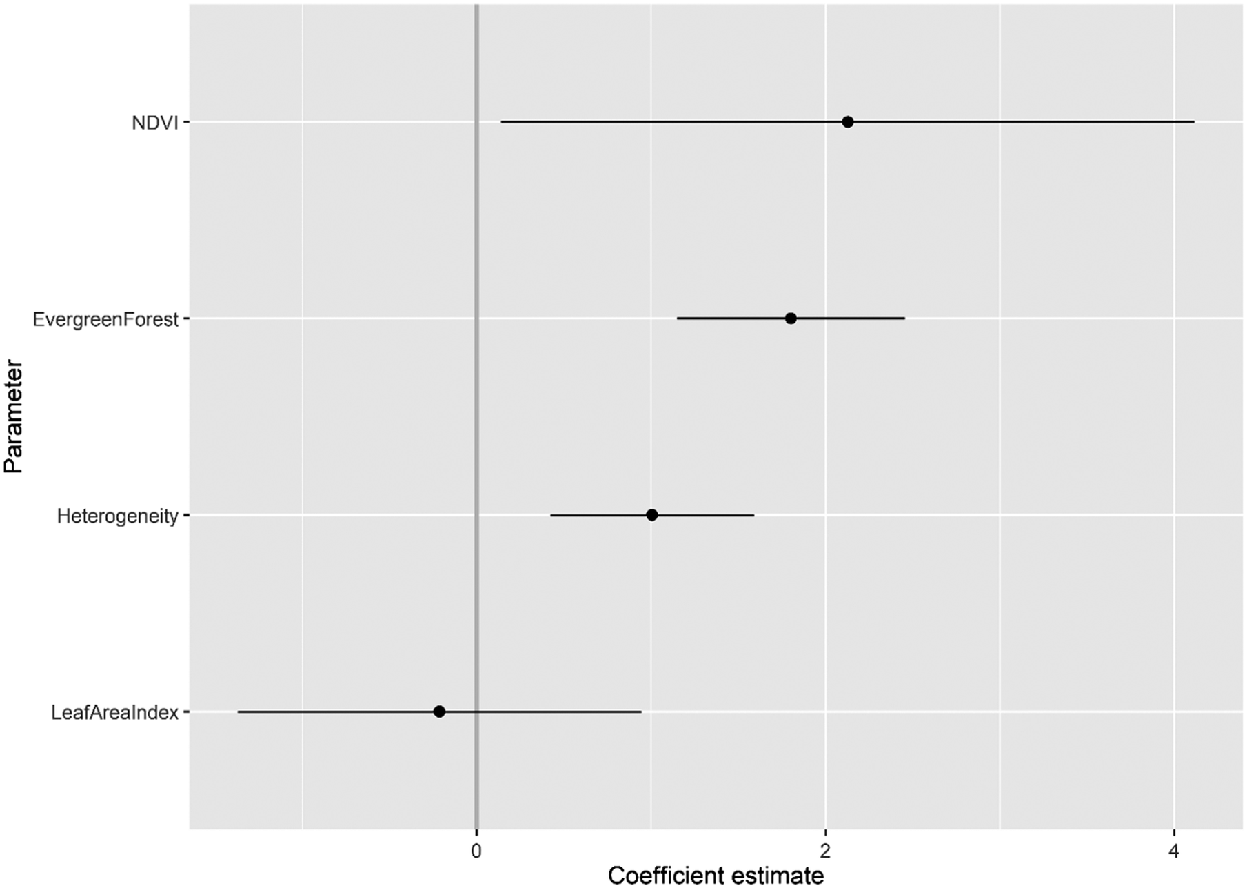
Figure 2. Coefficient estimates (with standard errors) for the best supported candidate logistic regression habitat covariate model (#6) for the Madagascar Serpent-eagle using Akaike’s Information Criterion corrected for small sample sizes.
SDMs
Three candidate SDMs had an ΔAICc ≤2, with the best supported penalised SDM using linear, quadratic, and hinge terms and a coefficient penalty β = 3 as model parameters (model 15, Table S3). The optimal SDM had high calibration accuracy (CBI = 0.835) and was robust against random expectations (pROC = 1.892, SD ± 0.058, range: 1.746–2.000). The largest continuous AOH extended along the remaining areas of tropical moist forest of the Eastern Malagasy Region in the Central and Eastern domains (Figure 3). A second substantial area of habitat was identified across the Masoala Peninsula and further north into forested, lower elevation areas of the Tsaratanana Massif.
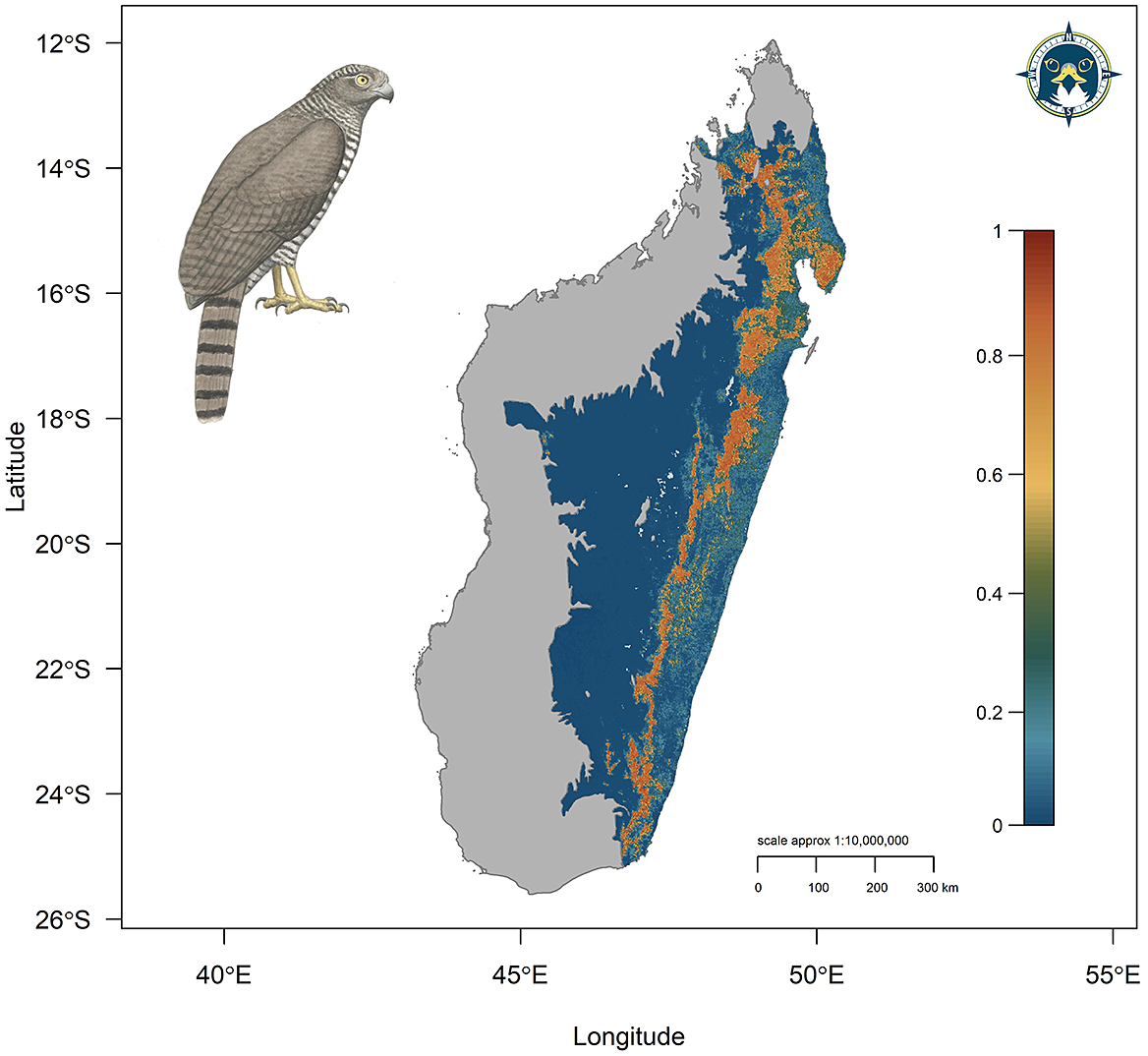
Figure 3. Continuous Species Distribution Model for the Madagascar Serpent-eagle using a penalised logistic regression model algorithm. Map denotes continuous prediction with red areas (values closer to 1) having highest habitat suitability, orange/yellow medium suitability, and blue/green low suitability.
The optimal model shrinkage penalty was able to retain four non-zero beta coefficients, setting to zero most model terms, meaning only a small subset of covariate terms were highly informative to model prediction (Figures S2–S4). From the penalised linear beta coefficients, the Madagascar Serpent-eagle was most positively associated with vegetation heterogeneity (β = 1.220), followed by NDVI (β = 0.148), Evergreen Forest (β = 0.043), and Leaf Area Index (β = 0.002). From the penalised response functions, peak suitability for vegetation heterogeneity was at 90–95%, with highest suitability for composite NDVI values >20 (Figure 4). The Madagascar Serpent-eagle was positively associated with >95% Evergreen Forest cover with a flat response to Leaf Area Index values between 0.0 and 3.0.
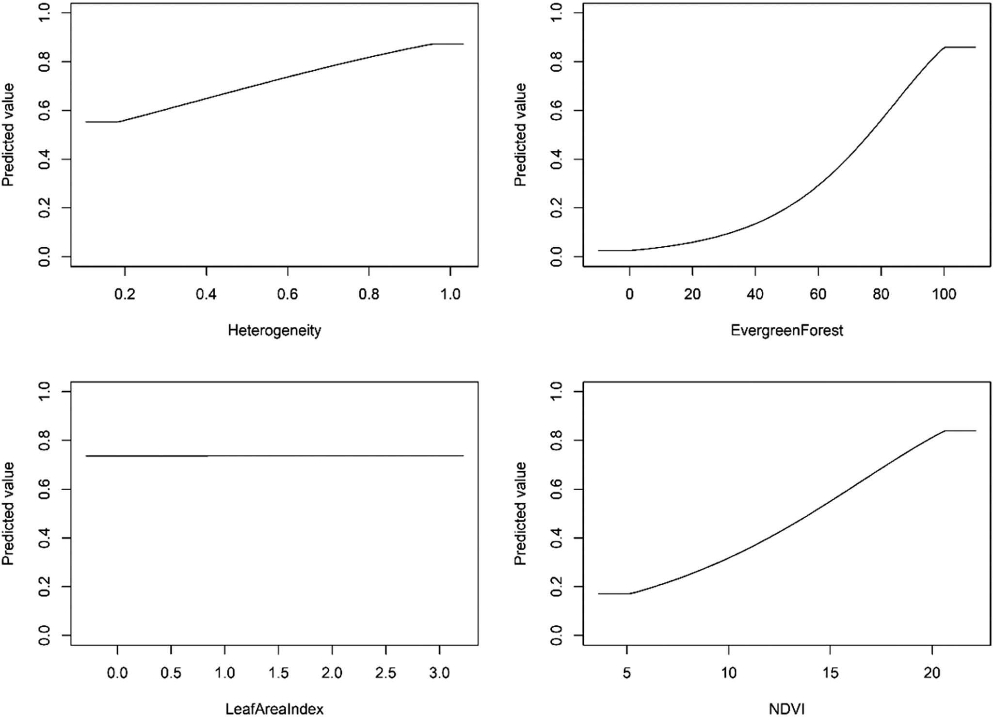
Figure 4. Penalised logistic regression response functions for each habitat covariate from the optimal Species Distribution Model for the Madagascar Serpent-eagle. The curves show the contribution to model prediction (y-axis) as a function of each continuous habitat covariate (x-axis). Maximum values in each response curve define the highest predicted relative suitability. The response curves reflect the partial dependence on predicted suitability for each covariate and the dependencies produced by interactions between the selected covariate and all other covariates.
Range metrics, population size, and protected area coverage
The reclassified binary model (maxTSS threshold = 0.670) calculated a model AOH = 30,121 km2, 13% less than the current IUCN range map area of 34,655 km2 (Figure 5). From the model AOH, maximum Extent of Occurrence = 397,293 km2 and minimum Extent of Occurrence = 281,736 km2 (Figure 5), with an Area of Occupancy = 79,520 km2. Using our formulation based on habitat area from nearest neighbour distances, we calculated that the model AOH could potentially support 533 mature individuals, or 267 breeding pairs, across the entire Madagascar Serpent-eagle range. The current protected area network covered 95% (28,654 km2) of the model AOH, 50% greater than the target protected area representation of 45% (Figure 6). Priority areas of habitat which are without protected area coverage in the protected area network were identified as: (1) a large area of forest at Alan’ i Fampanambo linking up to Ambotavoky Special Reserve; (2) a forest corridor 20 km west of Anosibe an’ala extending north from Marolambo National Park; (3) connecting Midongy Befotaka National Park with d’Andohahela National Park in the far south (Figure 6, blue circles).

Figure 5. Updated IUCN range metrics for the Madagascar Serpent-eagle showing the reclassified binary model Area of Habitat (brown) and Extent of Occurrence (hashed black polygon). Blue polygon defines current IUCN range map. Light grey polygons represent the species accessible area. Dark grey polygon defines the national boundary of Madagascar not within the species accessible area.

Figure 6. Protected area network coverage for the Madagascar Serpent-eagle showing the reclassified binary model Area of Habitat (brown) overlaid with the World Database on Protected Areas (WDPA) network (black-bordered polygons). Light grey polygons represent the species accessible area. The dark grey polygon defines the national boundary of Madagascar not within the species accessible area. Blue circles identify priority WDPA network coverage gaps: (1) Alan’ i Fampanambo forest and surrounding area north; (2) a forest corridor 20 km west of Anosibe an’ala extending north from Marolambo National Park; (3) a forest corridor connecting Midongy Befotaka National Park with Andohahela National Park.
Discussion
Raptors resident in developing countries with small geographical ranges that are forest dependent are particularly extinction prone and under-studied (Buechley et al. Reference Buechley, Santangeli, Girardello, Neate‐Clegg, Oleyar, McClure and Şekercioğlu2019). Additionally, tropical forest raptor species are more threatened compared with tropical non-forest raptors, mainly due to habitat alteration driven by logging and land clearance for agriculture (McClure et al. Reference McClure, Westrip, Johnson, Schulwitz, Virani, Davies, Symes, Wheatley, Thorstrom, Amar, Buij, Jones, Williams, Buechley and Butchart2018). This is further compounded for conservation action by the lack of fundamental biological information on tropical raptors in general (Buechley et al. Reference Buechley, Santangeli, Girardello, Neate‐Clegg, Oleyar, McClure and Şekercioğlu2019), required for underpinning the scientific understanding needed to effect policy and conservation action (McClure et al. Reference McClure, Westrip, Johnson, Schulwitz, Virani, Davies, Symes, Wheatley, Thorstrom, Amar, Buij, Jones, Williams, Buechley and Butchart2018). The Madagascar Serpent-eagle is thus a prime example of a raptor facing all these combined threats and knowledge gaps. Our results updated previous IUCN range metrics, with our AOH map predicting beyond the Madagascar Serpent-eagle known range. We estimated a population size of 533 mature individuals and that 95% of Madagascar Serpent-eagle AOH is currently protected. Additionally, we recommend three new protected areas for full habitat protection across the species range.
Species range metrics are a key component for assessing the conservation status and extinction risk of taxa on the IUCN Red List (IUCN 2019). Using model-based interpolation within our SDM framework we were able to extend the current known range of the Madagascar Serpent-eagle (BirdLife International 2016), predicting into an extensive area further south than the current IUCN range map (see Figure 5). However, despite this predicted range extension our AOH map closely matched that of the IUCN, albeit 13% less than the IUCN range area. We recommend that this updated range map is incorporated into the next Red List assessment for the Madagascar Serpent-eagle. In the meantime, exploratory surveys should be undertaken to assess model accuracy in this newly predicted habitat area, like previous SDMs used for rare taxa in Madagascar (Raxworthy et al. Reference Raxworthy, Martinez-Meyer, Horning, Nussbaum, Schneider, Ortega-Huerta and Peterson2003, Pearson et al. Reference Pearson, Raxworthy, Nakamura and Peterson2007).
Quantifying species–habitat associations is key to understanding species’ habitat requirements and environmental preferences (Matthiopoulos et al. Reference Matthiopoulos, Fieberg and Aarts2020, Sutton et al. Reference Sutton, Rene de Roland, Thorstrom and McClure2022). We identified the most parsimonious habitat variables based on our occurrence data fitted with multiple logistic regressions. Interestingly, including the Climatic Moisture Index resulted in the worst performing habitat covariate model (model 1) (Table 2), despite the assumption that climate is key to defining species range limits at broad scales (Pearson and Dawson Reference Pearson and Dawson2003). We suspect that vegetation indices such as NDVI, which can be strongly correlated with climatic conditions (Ichii et al. Reference Ichii, Kawabata and Yamaguchi2002, Pettorelli Reference Pettorelli2013), were better able to capture the broad scale tropical forest vegetation dynamics and thus habitat associations for the Madagascar Serpent-eagle. Similarly, topography was not as important when compared with biophysical measures such as Leaf Area Index and FPAR, with neither topographical covariate in the best supported models (see Table 2). Perhaps complex topography does not explain habitat associations as well as biophysical measures for those tropical forest taxa that inhabit less complex terrain at low to mid elevations.
From the penalised SDMs, our best model identified the strongest association with Heterogeneity (i.e. vegetation species richness) derived from the Enhanced Vegetation Index, followed by composite NDVI. This concurs with the Enhanced Vegetation Index being a more important biophysical measure than NDVI in dense tropical forests (Huete et al. Reference Huete, Didan, Miura, Rodriguez, Gao and Ferreira2002, Qiu et al. Reference Qiu, Yang, Wang and Su2018). We suspect this strong association with high vegetation species richness is possibly a proxy related to increased prey availability (i.e. chameleons and geckos) in vegetation-rich habitats (Hobi et al. Reference Hobi, Dubinin, Graham, Coops, Clayton, Pidgeon and Radeloff2017), which are thus more likely to be areas conserved for high biodiversity. Madagascar Serpent-eagles had a flat response up to Leaf Area Index values of 3.0 (see Figure 4), concurrent with the negative association in the best-fit habitat covariate model. This suggests a weak association between Madagascar Serpent-eagle distribution with Leaf Area Index values lower than expected from a global analysis (Asner et al. 2003), though this study did not include Madagascar. Perhaps the flat to negative association with Leaf Area Index was related to our low occurrence sample and further compounded by the inclusion of the evergreen forest landcover layer. Importantly, our penalised SDM was able to identify a strong positive association with >95% evergreen forest cover, concurrent with previous ground-based habitat associations for the species (Thorstrom and Rene de Roland Reference Thorstrom and Rene de Roland2000, Benjara et al. Reference Benjara, Rene de Roland, Rakotondratsima and Thorstrom2021).
Estimating population size is key for IUCN Red List assessments, because it is used in the criteria for designating the specific Red List threat category for a given taxon (IUCN 2019). Our estimate of 533 mature individuals based on predicted AOH is within the population size range currently given by the IUCN (250–999 mature individuals) (BirdLife International 2016). Our estimate would technically place the Madagascar Serpent-eagle in the Vulnerable category based on criterion D for a very small or restricted population (IUCN 2019). However, due to low breeding productivity (1 young every 2–3 years) (Thorstrom and Rene de Roland Reference Thorstrom and Rene de Roland2000), and possible high juvenile mortality (Benjara Reference Benjara2015, BirdLife International 2016), we are reluctant to recommend re-listing from Endangered to Vulnerable without first assessing population size from further ground-truthing surveys. Encouragingly, protected area coverage was very high, and we recommend consideration of the three major gaps we have identified here as new protected areas, further supported by exploratory surveys to confirm presence. Protected areas have been effective in preventing species extinctions (Geldmann et al. Reference Geldmann, Barnes, Coad, Craigie, Hockings and Burgess2013). Therefore, protecting as much Madagascar Serpent-eagle habitat as possible is key to its future survival as carried out previously in the Masoala Peninsula (Thorstrom and Rene de Roland Reference Thorstrom and Rene de Roland2000).
We recognise there are limitations to our approach regarding sample size, but we used the current best-practice modelling methodology combined with robust remote-sensing variables to calculate our baseline metrics. Even though unstructured occurrence data can have sampling bias (Beck et al. Reference Beck, Böller, Erhardt and Schwanghart2014), opportunistically collected presence-only data are often the only location data available and generally sample beyond the extent of the smaller spatial scale of systematic surveys (Sutton et al. Reference Sutton, McClure, Kini and Leonardi2020, Sutton & Puschendorf Reference Sutton and Puschendorf2020). Thus, when used in conjunction with a modelling framework designed to account for inherent spatial biases unstructured data can fill distributional knowledge gaps (Rhoden et al. Reference Rhoden, Peterman and Taylor2017, Sutton et al. Reference Sutton, Ibañez, Salvador, Taraya, Opiso, Senarillos and McClure2023b). However, obtaining further occurrences would be useful for improving our predictions and updating the baseline biological parameters set out here.
Madagascar has been identified as a priority region for raptor research and conservation due to its range of endemic, under-studied raptors (Buechley et al. Reference Buechley, Santangeli, Girardello, Neate‐Clegg, Oleyar, McClure and Şekercioğlu2019). Future modelling goals include predicting the core remaining areas of habitat for all Madagascar raptors to identify priority areas for current spatial conservation planning. Future work should thus focus on building upon the SDM framework set out here to estimate range metrics, population size, and protected area coverage for all Madagascar raptors combined with remote-sensing technology. Our model framework is a fast, cost-effective method to establish key spatial conservation baselines. This framework is widely applicable across all taxa but particularly for rare, under-studied species such as the Madagascar Serpent-eagle which faces threats to its future survival.
Supplementary Materials
To view supplementary material for this article, please visit http://doi.org/10.1017/S0959270922000508.
Acknowledgements
We thank all individuals and organisations who contributed occurrence data to the Global Raptor Impact Network information system. We thank the M. J. Murdock Charitable Trust for funding and technicians from The Peregrine Fund’s Madagascar Project for support and fieldwork: Ladoany Eugene, Moïse, and Monesy. We thank the associate editor Antoni Margalida and two anonymous reviewers for comments and suggestions that improved the manuscript.
LJS conceived the idea and designed the methodology; AB, LARR, and RT collected the data; LJS analysed the data and led the writing of the manuscript with supervision from CJWM. All authors contributed critically to the drafts and gave final approval for publication.
The raster and shapefile data that support this study are openly available on the data repository figshare https://doi.org/10.6084/m9.figshare.21318126.v1. Due to confidentiality of nest locations for this endangered species we are unable to publicly share our occurrence dataset.


