

I. INTRODUCTION
The Joint Video Exploration Team (JVET for short) is formed by a group of experts from both ITU-T VCEG and ISO/IEC MPEG organizations. In recent years, research efforts for developing the next generation video code have been accumulated by this group. The targeted applications for this new standard initiative include standard dynamic range video, VR/360 video, and high dynamic range video. In April 2018, a new video coding standard named Versatile Video Coding (VVC) has been kicked off, based on the responses of the Call for Proposals (Cfp) [Reference Segall, Baroncini, Boyce, Chen and Suzuki1]. The committee that is responsible for the VVC standard development is then renamed as Joint Video Experts Team (JVET for short).
The adoption in the first version of the VVC standard working draft and its reference software, VTM-1 [2], contains only block structure partitioning improvements beyond the HEVC standard [3,Reference Sullivan, Ohm, Han and Wiegand4]. Using that as a starting point, coding tools in various aspects are further evaluated, among which many have been well studied in the past few years in the exploration phase of the new standard. For the study of tool interactions, coding tools that have been studied in the past but not yet been adopted into VVC/VTM are integrated into a secondary reference software – benchmark set (BMS) [5]. The BMS software is built on top of the VTM software by adding some promising coding tools to it. In this paper, an overview is presented for the new video coding technologies that have been either included in the reference software VTM-2 or the associated BMS-2 software. The purpose of such a summary is to demonstrate the potential capability of the new standard up to some point. It is at the early stage of the VVC standard development. Further investigation and improvement in coding efficiency are expected before October 2020, which is set to be the finalization date of the first release of the VVC standard.
The rest of this paper is organized as follows: Section II gives an overview of the structure of the VVC standard development; Section III discusses in details the new coding tools that have been adopted in the VVC standard working draft 2 and the VTM-2 software; Section IV discusses in details the new coding tools that have been included in the BMS-2 software; in Section V, simulation results are presented to demonstrate the status of the new standard progress collectively and individual performance of coding tools in the BMS-2 software; Section V concludes the paper.
II. OVERVIEW OF THE VVC STANDARD DEVELOPMENT
The basic function modules in the VVC standard design follow the traditional hybrid block-based coding structure, such as block-based motion compensation, intra prediction, transform and quantization, entropy coding, and loop filtering. These are similar to those ones that were used in the HEVC standard. The improvements of coding efficiency in the VVC standard beyond its predecessor come from the following several aspects:
A) More flexible block partitioning structures
Under the root of a coding tree unit (CTU), which is a square two-dimensional array of up to 128 × 128 luma samples, a coding block can be firstly split into four smaller square child coding blocks of equal size recursively. A coding block can later be split into two children coding blocks of equal size using binary-tree (BT) split or into three children coding blocks of unequal sizes using ternary-tree (TT) split. These flexible splitting structures enable the quick adaptation of coding block size into various video contents.
B) Sub-block-based motion compensation
Traditionally, each prediction unit (PU) of an inter coded coding block contains independent motion information, such as motion vector(s) and information related to the reference picture(s). Sub-block-based motion compensation partitions a coding block into a number of sub-blocks, each of which may still have different motion information. The benefit of having sub-block-based motion compensation lies in (1) the partitioning from current coding block into its sub-blocks is fixed (the sub-block size is fixed) without the need to indicate the partition structure and depth; (2) the motion information for each sub-block is derived instead of being signaled. In this way, the signaling overhead of representing a set of different motion information for a coding block can be avoided. Currently the sub-block size for affine motion compensation is 4 × 4 and 8 × 8 luma samples for sub-block-based temporal motion vector prediction mode.
C) Advanced post filtering
In addition to the existing in-loop filtering tools such as deblocking filter and SAO filter, the previously studied adaptive loop filter (ALF) during the HEVC development has been included into the VVC standard with further improvements.
D) Finer granularity in prediction precision
In intra prediction, the number of intra prediction modes is expanded from 35 to 67. In addition to that, for each position in the prediction block, the prediction signal may be adjusted. In inter coding, in addition to various block shapes resulting from the flexible block partitions, the highest accuracy of a luma motion vector is increased from 1/4-pel to 1/16-pel; the corresponding chroma motion vector accuracy is increased from 1/16-pel to 1/32-pel.
E) More adaptation in transformation and quantization
The residue signal will go through different transforms adaptively. For the transform design, a number of different transform cores are provided. The index of selection will be signaled. A mechanism called dependent quantization is used to adaptively switch between two different quantizers such that the quantization error can be reduced.
F) Screen content coding support
Screen content video is considered as a very important target application in the VVC standard. Coding tools that are efficient for compressing the screen content materials have been evaluated, such as the current picture referencing (CPR; or by another name intra block copy (IBC)) mode.
In the following two sections, details of these new features in the VVC standard will be discussed.
III. NEW CODING TOOLS IN VTM SOFTWARE
In this section, a number of new coding tools that have been adopted into the VVC working draft and VTM software are reviewed. The discussed items in this paper do not form a complete list of adoptions in the new standard. For more details of each tool in the VVC standard, [Reference Chen, Ye and Kim6] can be referred.
A) Block partition structure: quad-tree plus multi-type tree
In the VVC working draft 2 [Reference Bross, Chen and Liu7], a block partitioning strategy called quad-tree + multi-type tree (QT + MTT for short) [Reference Li8] is used. Each picture is divided into an array of non-overlapped CTUs. A CTU is a two-dimensional array of pixels with 128 × 128 luma samples (and corresponding chroma samples), which can be split into one or more coding units (CU) using one or a combination of the following tree-splitting methods:
1) Quaternary-tree split as in HEVC
This splitting method is the same as in HEVC, each parent block is split in half in both horizontal and vertical directions. The resulting four smaller partitions are in the same aspect ratio as its parent block. In VVC, a CTU is firstly split by quaternary-tree (QT) (recursively). Each QT leaf node (in square shape) can be further split (recursively) using the multi-type (BT and TT) tree as below:
2) BT split
This splitting method refers to dividing the parent block in half in the either horizontal or vertical direction [Reference An, Chen, Zhang, Huang, Huang and Lei9,Reference An, Huang, Zhang, Huang and Lei10]. The resulting two smaller partitions are half in size as compared to the parent block.
3) TT split
This splitting method refers to dividing the parent block into three parts in the either horizontal or vertical direction in a symmetrical way [Reference Li8]. The middle part of the three is twice as large as the other two parts. The resulting three smaller partitions are 1/4, 1/2, and 1/4 in size as compared to the parent block.
Illustrations of BT and TT are shown in Fig. 1. In VVC, a CU is a leaf node of block partitioning result without further splitting. Its PU and transform unit (TU) are of the same size as the CU unless the CU size exceeds the maximum TU size (in which case the residues will be split until maximum TU size is reached). This is different from HEVC, where PU and TU can be smaller than its CU in general. The block partitioning operation is constrained by the maximum number of splits allowed (split depth) from the CTU root and the minimum block height and width for a leaf CU. Currently, the smallest CU size is 4 × 4 in luma samples. An example of block partitioning results of a CTU is shown in Fig. 2.

Fig. 1. Binary splits and ternary splits of a parent block.
Fig. 2. Example of a CTU block partition results using quad-tree plus multi-type tree structure.
Besides these flexible block partitioning options, for coding of an intra slice, the coding tree structures for luma samples and chroma samples of the CTU can be different (referred as dual-tree structure). In other words, chroma samples will have an independent coding tree block structure from the collocated luma samples in the same CTU. In general, this allows chroma samples to have larger coding block sizes than luma samples.
B) Intra prediction
1) Sixty-seven intra prediction modes
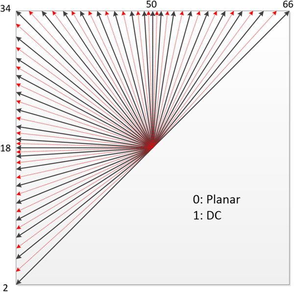
The number of intra directional prediction modes is extended from 33 in HEVC to 65 in VVC [Reference Choi, Piao, Choi and Kim11]. In Fig. 3, an illustration of the increased directions is shown. In addition to that, DC and planar modes are still in use. For DC mode, only samples in the longer side are used to calculate the average DC value in the non-square block, to avoid division operation. Similar as in HEVC, the intra mode coding involves two parts: three MPM modes from spatial neighbors and 64 non-MPM modes using six-bit fixed length coding.

Fig. 3. Sixty-seven intra prediction modes.
2) Wide-angle prediction for non-square blocks
For non-square blocks, some of the traditional intra prediction modes are adaptively replaced by wide-angle directions, keeping the total number of intra prediction modes unchanged (67) [Reference Racape12]. The new prediction directions for non-square blocks are shown in Fig. 4, where the block width is smaller than block height. In general, more modes will be coming from the longer side of the block. In the case in Fig. 4, some modes near the top-right angular mode (mode 66 in Fig. 3) are replaced by additional angular mode below the bottom-left angular mode (mode 2 in Fig. 3). To support these prediction directions, the top reference with length 2W + 1, and the left reference with length 2H + 1, are defined as shown in Fig. 4.

Fig. 4. Reference samples for wide-angular intra prediction (width < height).
3) Position-dependent prediction combination
Position-dependent prediction combination (PDPC) combines intra prediction with position-dependent weighting of some top and reference samples [Reference Said, Zhao, Chen, Karczewicz, Chien and Zhou13,Reference Van der Auwera, Seregin, Said, Ramasubramonian and Karczewicz14]. PDPC is applied to the following intra modes: planar/DC, horizontal/vertical, diagonals (2, 66), and four adjacent modes. The pixel at (x, y) position is predicted as in (1):
 $$\eqalign{P\lpar x\comma \; y\rpar & = \lpar wL\times R_{-1\comma y} + wT \times R_{x\comma -1} - wTL\times R_{-1\comma -1} \cr & \quad + \lpar {64-wL-wT+wTL} \rpar \times P\lpar {x\comma \; y} \rpar +32 \rpar \gg 6} $$
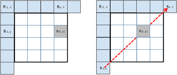
where R −1,−1 is the top-left corner reference sample; R −1, y and R x,−1 are two reference samples from the left and top reference lines. For DC, planar, vertical, and horizontal modes, they are to the left and on top relative to the current pixel position, as shown in Fig. 5; for other angular modes, the two reference samples are selected according to the prediction direction, as shown in Fig. 5. PDPC is applied to the following intra modes without signaling: planar, DC, horizontal, vertical, bottom-left angular mode and its eight adjacent angular modes, and top-right angular mode and its eight adjacent angular modes.

Fig. 5. Top and left reference samples in PDPC for DC/planar/vertical/horizontal modes (left) and other angular modes (right).
4) Cross component linear model
Cross-component linear model (CCLM) utilizes a linear prediction model from luma samples to chroma samples, as follows [Reference Ma, Yang and Chen15]:
 $$pred_C \lpar {i\comma \; j} \rpar =\alpha \cdot re{c}'_L \lpar {i\comma \; j} \rpar +\beta $$
where pred C is the chroma sample predictor at (i, j) in a CU and re c′L is the down-sampled reconstructed luma samples of the same location. Parameters α and β are derived by minimizing the regression error between the neighboring reconstructed luma (down-sampled) and chroma samples (left one column and top one row) around the current block. CCLM can reduce the redundancy among different color components.
C) Inter prediction
1) Affine motion compensation
Traditional affine motion model consists of six parameters [Reference Lin, Chen, Zhang, Maxim, Yang and Zhou16,Reference Chen, Yang and Chen17]. For each pixel at location (x, y) with the given affine mode, its motion vector (v x, v y) can be linearly interpolated by the three corner control point motion vectors, as is shown in the left side of Fig. 6.

Fig. 6. Six-parameter affine model versus four-parameter affine model.
A simplified version of affine mode is also considered, where only four parameters (or equivalent motion vectors at two control point locations) are required to describe the motions in an affine object, as is shown in the right side of Fig. 6. In this case, the motion vector at location (x, y) can be expressed by using the motion vectors at the top left and top right corners, as is in formula (3). According to this formulation, the motion vector of each pixel inside the current block will be calculated as a weighted average of the two (or three, in case of six-parameter) corner control points' motion vectors. In VVC standard, a CU level flag is used to switch between four-parameter affine mode and six-parameter affine mode.
 $$\left\{\matrix{{v_x =\displaystyle{{\lpar v_{1x} -v_{0x} \rpar }\over{w}}x-\displaystyle{{\lpar v_{1y} -v_{0y} \rpar }\over{w}}y+v_{0x}} \cr {v_y =\displaystyle{{\lpar v_{1y} -v_{0y} \rpar }\over{w}}x+\displaystyle{{\lpar v_{1x} -v_{0x} \rpar }\over{w}}y+v_{0y}}}\right. $$
Although each sample in an affine coded block may derive its own motion vector using the above formula, actually the affine motion compensation in VVC standard operates on a sub-block basis to reduce the complexity in implementation. That is, each 4 × 4 luma region in the current CU will be considered as a whole unit (using the center location of this sub-block as the representative location) to derive its sub-block motion vector. To improve the precision of affine motion compensation, 1/16-pel luma MV resolution and 1/32-chroma MV resolution are used.
For an affine coded block, its control point motion vectors (CPMVs) can be predicted by derivation from a neighboring affine coded block. Assuming the neighboring block and the current block are in the same affine object, the current block's CPMVs can be derived using the neighboring block's CPMV plus the distance between them. This prediction is referred as the derived affine prediction. The CPMVs of an affine coded block can also be predicted by the MVs from each corner's spatial neighboring coded blocks. This prediction is referred as the constructed affine prediction.
After the prediction, for each CPMV of the current block, the prediction differences are subject to entropy coding, in the same way of regular inter MVD coding. In affine case, for each prediction list, up to three MV differences per reference list will be coded.
Note: affine mode with signaled MV difference is included in VTM-2. Affine merge mode using the candidates from both the derived prediction and the constructed prediction is later adopted in VTM-3.
2) Adaptive motion vector resolution
For each coding block with a signaled non-zero motion vector difference, the resolution of the difference can be chosen from one of the three options: {1/4-pel, 1-pel, 4-pel} [Reference Zhang, Han, Chen, Hung, Chien and Karczewicz18]. For the latter two, the decoded difference should be left shifted by 2 or 4 separately, before adding them to the MV predictor. At the meantime, the resolution of the associated MV predictor will be rounded to the same resolution as the corresponding MV difference. By using adaptive motion vector resolution, the coding cost for larger MV values can be reduced. This tool is especially efficient when the coded video is in high resolution.
3) Alternative temporal MV prediction
Alternative temporal MV prediction is a merge mode with sub-block granularity [Reference Chien and Karczewicz19,Reference Xiu20]. At CU level, the motion vector from the first available merge candidate is used to find the current block's collocated block in the collocated reference picture. This motion vector is referred as CU level MV offset. The current block is then divided into sub-blocks with 8 × 8 luma samples in size. For each sub-block, its motion vector (if applicable) comes from the collocated sub-block in the collocated block found for current CU. The CU level motion vector offset will be used for a sub-block if its collocated sub-block is not coded in regular inter mode (without a temporal MV).
D) Transformation
In VVC, large block-size transforms, up to 64 × 64 in size, are supported. In addition to this change, the following features are added:
1) Zero-out high-frequency coefficients
If the width of a transform block is 64, then only the left 32 columns of coefficients will be kept (the rest will be assumed to be zero). Similarly, if the height of a transform block is 64, only the top 32 rows of coefficients will be kept.
2) Multiple transforms selection
Besides DCT-II in HEVC, DST-VII and DCT-VIII can be selected for residue coding in intra and inter coded blocks [Reference Choi, Park and Kim21]. In Table 1, the selection and signaling of multiple transforms selection (MTS) are shown.
Table 1. Transform and signaling mapping table.
E) Quantization and coefficient coding
1) Sign data hiding
Currently, sign data hiding design is the same as in HEVC.
2) Dependent quantization
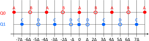
Transform coefficient levels are to be quantized. In VVC, there are two scalar quantizers used, denoted by Q0 and Q1, as illustrated in Fig. 7 [Reference Schwarz, Nguyen, Marpe and Wiegand22]. The location of the available reconstruction levels is specified by a quantization step size Δ. For each coefficient, the selection of scalar quantizer (Q0 or Q1) is not signaled in the bitstream but determined by the parities of the transform coefficient levels that precede the current transform coefficient in encoding/decoding order. Depending on the parities of transform coefficients, one of four states will be located. For states 0 and 1, Q0 will be used; for states 2 and 3, Q1 will be used. For each transform coefficient, the current state and next state(s) are specified in Table 2, where k represents the current transform coefficient level. At the beginning of coefficient coding, the state is set equal to 0.

Fig. 7. Two scalar quantizers used in dependent quantization.
Table 2. The quantizer selection and state transit for dependent quantization.
Note that the above two methods cannot be turned on simultaneously.
F) In-loop filtering
1) Adaptive loop filter
ALF was proposed during the development of the HEVC standard [Reference Karczewicz, Zhang, Chien and Li23,Reference Karczewicz, Shlyakhov, Hu, Seregin and Chien24]. Compared to that version, the adopted ALF in the VVC standard has the following features:
(1) Filter shape: a 7 × 7 diamond shape filter (with 13 different coefficients) is applied to luma blocks and a 5 × 5 (with seven different coefficients) diamond shape filter is applied to chroma blocks
(2) Block classification: each 4 × 4 luma block is categorized into one of 25 different classes, using the vertical, horizontal, and two diagonal gradients. Therefore, up to 25 sets of luma filter coefficients will be signaled.
(3) Geometry transformation of filter coefficients: for each 4 × 4 luma block, depending on the calculated gradients, the filter coefficients may go through one of the three transformations: diagonal, vertical flip, and rotation, before applying them to the samples.
From the decoder side, the ALF filtering process is performed such that each sample R(i, j) within the CU is filtered, resulting in sample value R′(i, j) as shown below in formula (4), where L denotes filter length, f m, n represents filter coefficient, and f(k, l) denotes the decoded filter coefficients:
 $$R^{\prime} \lpar {i\comma \; j}\rpar = \sum_{k = - \lpar L/2\rpar }^{L/2} \sum_{l = - \lpar L/2\rpar }^{L/2} f \lpar k\comma \; l\rpar \times R\lpar i + k\comma \; j + l\rpar + 64 \gg 7 $$
IV. TOOLS DEVELOPMENT IN BMS SOFTWARE
In this section, coding tools that have been included in the BMS-2 software are discussed. For most tools, a variation of them is later adopted into the VTM software and VVC standard working draft.
A) CPR or IBC
One of the requirements for VVC standard development is to provide good support for coding screen content materials [Reference Xu, Li, Li and Liu25]. In HEVC SCC extensions [Reference Liu, Xu, Lei and Jou26], screen coding tools have been studied. By evaluating the coding performance improvement and the implementation complexity, CPR mode in the HEVC SCC extensions [Reference Xu27] has been reported to be efficient in coding screen content materials while its operations are most aligned with existing building blocks of the HEVC design.
In the CPR mode [Reference Xu, Li, Li and Liu25] of the BMS-2 software, the current (partially) decoded picture is treated as a reference picture. By referring to such a reference picture, the current block can be predicted from a reference block of the same picture, in the same manner as motion compensation. The differences for a CPR coded block from the normal MC include the followings:
(1) Block vectors (the displacement vector in CPR) have only integer resolution, no interpolation needed for luma or chroma.
(2) Block vectors are not involved in temporal motion vector prediction.
(3) Block vectors and motion vectors are not used to predict each other.
(4) A valid block vector has some constraints such that it can only point to a subset of the current picture. To reduce the implementation cost, the reference samples for CPR mode should be from the already reconstructed part of the current slice or tile and should meet the WPP parallel processing conditions.
Note: CPR mode is later adopted into the VTM-3 software with its available search range constrained within the current CTU [Reference Xu, Li and Liu28].
B) Non-separable secondary transform
After the above (primary) transform, a secondary transform can be applied to the top-left corner of the transform coefficients matrix [Reference Zhao, Chen and Karczewicz29]. This transform core is non-separable and is applied only to residues of intra coded blocks. Depending on the intra prediction mode used, one non-separable secondary transform (NSST) transform will be selected from a set of different predefine NSST cores. To limit the complexity of this tool, only 4 × 4 NSST (the 4 × 4 top-left corner of the coefficient block after primary transform) is adopted in the BMS-2 software. For each 4 × 4 NSST transform, 16 multiplications/coefficient are required.
Note: A simplified version of NSST is later adopted into the VTM-5 software.
C) Bi-directional optical flow or BIO
Bi-directional optical flow (BDOF) or BIO is a sample-wise motion refinement on the top of block-wise motion compensation for “true” bi-directional prediction, which means, one of the two reference pictures is prior to the current picture in display order and the other is after the current picture in display order [Reference Xiu30]. BDOF is built on the assumption of the continuous optical flow across the time domain in the local vicinity. It is only applied to the luma component.
The motion vector field (v x, v y) is determined by minimizing the difference Δ between the values in points A and B of the two reference pictures, as is shown in (5):
 $$\lpar v_x \comma \; v_y \rpar = \mathop {arg\min }\limits_{v_x \comma v_y } \sum_{[i^{\prime}\comma j\rsqb \in \Omega} {\Delta ^2 \lsqb i^{\prime}\comma \; j^{\prime}]}$$
 $$\eqalign{\Delta & =\lpar I^{\lpar 0\rpar }-I^{\lpar 1\rpar }_0+\nu_x\lpar \tau_1\partial I^{\lpar 1\rpar }/\partial x+\tau_0\partial I^{\lpar 0\rpar }/\partial x\rpar \cr & \quad + \nu_y\lpar \tau_1\partial I^{\lpar 1\rpar }/\partial y+\tau_0\partial I^{\lpar 0\rpar }/\partial y\rpar \rpar } $$
The definition of Δ is shown in (6), where, I 0 and I 1 are the luma sample values from reference picture 0 and 1, respectively, after block motion compensation. τ0 and τ1 denote the distances to the reference picture 0 and 1 from the current picture. ∂I (k)/∂x and ∂I (k)/∂y (k = 0, 1) represent the horizontal and vertical gradients at location (i′, j′), which represents all the points in a 3 × 3 square window Ω centered on the currently predicted point (i, j).
BDOF requires the decoder side to perform more complex operations than the traditional motion compensation. It was reported that 13 multiplications/samples are required for performing BDOF operation. The decoder runtime increase on top of VTM is 23% (RA config.). An illustration of BDOF is shown in Fig. 8.

Fig. 8. Illustration of BDOF.
Note: A simplified version of BDOF is later adopted into the VTM-3 software.
D) Generalized bi-prediction
In bi-directional prediction, the two prediction blocks are derived from two reference pictures and averaged (using equal weights) together to form the final prediction signal for the current coding block [Reference Su, Chuang, Chen, Huang and Lei31]. In generalized bi-prediction (GBi), in addition to this average weight (1/2 for each predictor), another four possible weights {-1/4, 3/8, 5/8, 5/4} may be used. A CU level flag is used to signal the usage of GBi when the bi-directional prediction is used. In addition, the weight index as listed in Table 3 will be sent.
Table 3. Binarization of GBi index.
In merge mode, the GBi weights are inherited from the selected merge candidate. In the residue (non-merge) mode, the weights are explicitly signaled. In Table 3, each listed weight w 1 is for one prediction list, the other weight is defined as w 2 = 1 − w 1. If the POC number of the current picture is in between the two reference pictures' POC numbers, only the middle three weights are considered (no negative weights).
Note: GBi is later adopted into the VTM-3 software.
E) Decoder side MV refinement
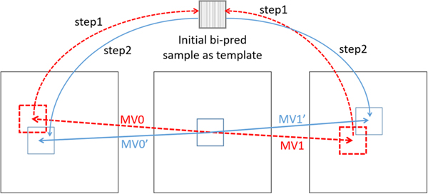
Decoder side MV refinement (DMVR) applies to bi-predictive merge candidates [Reference Chen, An and Zheng32]. In Fig. 9, the initial MV pair (MV0 and MV1) is suggested by the selected merge candidate. A pair of prediction blocks is generated by using the initial MV pair from the merge candidate. A template block is generated by averaging these two prediction blocks. Using this template, for each of the predictions lists, template matching costs between the generated template block and the reference block indicated by each of the eight neighboring positions around the original MV are checked. The position with a minimum cost is indicated as MV0′ (MV1′). This updated MV pair will be used to generate the final prediction signal.

Fig. 9. Illustration of DMVR.
Note: A simplified version of DMVR is later adopted into the VTM-4 software.
V. SIMULATION RESULTS
In this section, simulation results are provided to evaluate the coding performance of the latest VVC working draft as compared to the HEVC standard. To achieve that, results generated by the VVC reference software VTM-1, VTM-2, and BMS-2 are compared with those by the HEVC reference software HM-16.18 [33]. All the simulations are conducted under the VVC common test conditions as described in [Reference Bossen, Boyce, Li, Seregin and Sühring34]. The result differences are measured in BD rates [Reference Bjontegaard35] based on the calculations from four QP points, 22, 27, 32, and 37.
For the testing materials, a set of camera-captured sequences (Class A to E) and screen content sequences (Class F) defined in [Reference Bossen, Boyce, Li, Seregin and Sühring34] are used. Details of these test sequences can be found in Table 4. Class A (A1 and A2) sequences are with 3840 × 2160 resolution; Class B sequences are with 1920 × 1080 resolution; Class C sequences are with 832 × 480 resolution; Class E sequences are with 1280 × 720 resolution. Class F sequences have a set of mixed resolutions. Specifically, ArenaOfValor is with 1920 × 1080 resolution; BasketballDrillText is with 832 × 480 resolution; SlideEditing and SlideShow are with 1280 × 720 resolution. The average results of Class A1, A2, B, C, E are referred as “overall” in the subsequent tables.
Table 4. Test sequences in VVC CTC.
Table 5 shows the relative coding efficiency improvements of the VTM-1, VTM-2, and BMS-2 software as compared to HM-16.18 software. From this table, we can see that the structure-only improvements (QT + MTT) can provide roughly 4%/8%/8% gain for AI/RA/LB configurations, respectively. On top of that, another 14%/15%/10% gain can be achieved by adopting new coding tools into VTM-2 software, for AI/RA/LB configurations, respectively. The collective gains for VTM-2 over HM-16.18 software are 18%/23%/18% for AI/RA/LB configurations, respectively. By adding the tools in BMS-2 software as is on top of VTM-2, another 1%/3%/1% gain can be achieved for AI/RA/LB configurations, respectively.
Table 5. Performance comparison between VTM, BMS, and HM (HM-16.18 used as an anchor).
Table 5 also shows the complexity aspect of the comparisons. With the block structure improvements over the HEVC standard, the VTM encoder runs more than two times as slow as compared to the HM encoder in RA configuration. In addition, with the adopted new tools in VVC standard, the runtime of VTM-2 becomes more than three times as compared to the HM software. If the new tools in the BMS software are also considered, the runtime increase will be even more significant. On the other hand, the increase in decoder runtime is relatively moderate for VTM-1 and VTM-2 as compared to the HM software. With the inclusion of the decoder side operations in the BMS tools, the decoder runtime increase in the BMS software is more evident.
Note that the decoder runtime might not be a good measurement for a decoder's complexity. For example, 81% decoder runtime does not necessarily mean that the VTM-1 decoder is simpler than the HM decoder. The two should be however similar by analyzing their design complexity. One factor to contribute the difference would be the software optimization used in VTM codebase, such as data parallel processing using SIMD instructions. Higher percentage of large block sizes usage may also contribute to the decoder runtime decrease.
Table 5 also shows the screen content coding capability by including Class F results. For an encoder without having specific screen content coding tools support (CPR), the improvement in this class over HM is even lower than the overall average. With the CPR mode enabled in the BMS-2 software, a significant additional improvement (~16%) in coding efficiency for Class F can be achieved.
In addition to the overall improvements that the BMS-2 software added over VTM-2, Table 6 shows the relative coding efficiency improvements of individual tools in the BMS-2 software as compared to VTM-1 software. Among those tools, GBi, BDOF, and DMVR are beneficial for bi-directional prediction only. Therefore, the improvement of coding efficiency from these tools will be mainly in RA configurations. From the (RA) results, we can see that these tools provide decent compression benefits, but the complexity increases at the encoder and/or decoder sides are significant and should also be taken into consideration. Actually, the complexity is one of the major issues for these tools to be included in the VVC standard working draft. In a simplified variation, all the tools in the BMS-2 software are adopted into the VTM software and VVC standard draft text in a later stage.
Table 6. RA performance improvements of individual BMS tools over VTM-1

VI. CONCLUSION
The research and development efforts for the new video coding standard were actually initiated a few years before the establishment of JVET and its reference software JEM. A number of responses to the VVC Cfp showed that about 35–40% improvements in coding efficiency beyond the HEVC standard can be reached. However, many elements inside those responses, such as neural network-based approaches, may not be practical for the immediate standardization. In a short period after the first formal VVC standard meeting, the BMS-2 software has already shown a 26% BD rate savings over the previous standard. It is believable that further substantial improvements will be anticipated as the standardization progress evolves.
Xiaozhong Xu has been with Tencent since 2017 as a Principal Researcher. Prior to joining Tencent, he was with MediaTek (USA) from 2013 to 2017, as a Department Manager/Senior Staff Engineer. He was with Zenverge, Inc. (now part of NXP), as a Staff Software Engineer working on multi-channel video transcoding ASIC design, from 2011 to 2013. He also held technical positions at Thomson Corporate Research (now Technicolor) and Mitsubishi Electric Research Laboratories. Dr. Xu received his B.S. and Ph.D. degrees from Tsinghua University, Beijing, China, and the M.S. degree from Polytechnic School of Engineering, New York University, NY, all in Electrical Engineering. He is an active participant in video coding standardization activities since 2004. He has made extensive and successful contributions to various standards, including H.264/AVC, AVS (China), H.265/HEVC and its extensions, and the ongoing VVC standard.
Shan Liu is a Distinguished Scientist and General Manager at Tencent where she heads the Tencent Media Lab. Prior to joining Tencent she was the Chief Scientist and Head of America Media Lab at Futurewei Technologies. She was formerly Director of Multimedia Technology Division at MediaTek USA. She was also formerly with MERL, Sony, and IBM. Dr. Liu is the inventor of more than 200 US and global patent applications and the author of more than 50 journal and conference articles. She actively contributes to international standards such as VVC, H.265/HEVC, DASH, OMAF, and served as a co-Editor of H.265/HEVC v4 and VVC. She was in technical and organizing committees, or an invited speaker, at various international conferences including ICIP, VCIP, ICNC, ICME, MIPR, and ACM Multimedia. She served in Industrial Relationship Committee of IEEE Signal Processing Society 2014–2015 and was appointed the VP of Industrial Relations and Development of Asia-Pacific Signal and Information Processing Association (APSIPA) 2016–2017. Dr. Liu obtained her B.Eng. degree in Electronics Engineering from Tsinghua University, Beijing, China and the M.S. and Ph.D. degrees in Electrical Engineering from the University of Southern California, Los Angeles, USA.


 Open access