


I. INTRODUCTION
Stereo matching plays an essential role in computer vision tasks, including autonomous driving [Reference Chenyi, Ari, Alain and Jianxiong1, Reference Korbinian, Teodor, Felix, Heiko and Michael2], object detection and recognition [Reference Chen3, Reference Zhang, Li, Cheng, Cai, Chao and Rui4], and 3D reconstruction and understanding [Reference Yao, Luo, Li, Fang and Quan5–Reference Li, Dai and He7]. For a couple of rectified stereo images, disparity refers to the apparent pixel difference or motion between a pair of corresponding pixels on the left and right images [Reference Hamzah, Ibrahim and Abu Hassan8, Reference Hirschmüller9].
The dense disparity map estimation methods have been studied for many years. For the traditional stereo matching methods (e.g. semi-global matching (SGM) [Reference Hirschmüller9], non-local cost aggregation [Reference Yang10], second-order smoothness priors [Reference Woodford, Torr, Reid and Fitzgibbon11]), the classical pipeline involves the finding of corresponding points by matching cost, cost aggregation, optimization, disparity refinement, and post-processing based on the local or global features. In general, the traditional methods often focus on using the prior knowledge of images to construct the warping function through for improving matching accuracy.
For disparity prediction based on deep learning, recent efforts have yielded many high-quality outputs due to deep fully convolutional neural networks (FCN) [Reference Laina, Rupprecht, Belagiannis, Tombari and Navab12, Reference Kendall, Martirosyan, Dasgupta and Henry13] and a large amount of training data [Reference Mayer14–Reference Menze and Geiger16]. Classically, mainstream methods contain a four-step pipeline, while each step is important to the overall matching performance: 2D feature extraction, cost volume construction, 3D feature matching, and disparity regression [Reference Kendall, Martirosyan, Dasgupta and Henry13, Reference Zbontar and LeCun17, Reference Guo, Yang, Yang, Wang and Li18]. Zbontar and LeCun first calculated the matching costs by convolutional neural networks (CNNs) to improve the performance, and the result showed that CNNs could learn more robust features from images and produced reliable matching cost in this task [Reference Zbontar and LeCun17]. Following this work, many researchers [Reference Kendall, Martirosyan, Dasgupta and Henry13, Reference Zagoruyko and Komodakis19–Reference Yin, Darrell and Yu22] proposed several methods to improve matching accuracy [Reference Kendall, Martirosyan, Dasgupta and Henry13, Reference Yin, Darrell and Yu22], reduce some parameters [Reference Guo, Yang, Yang, Wang and Li18], or achieve self-supervision ability [Reference Zhong, Dai and Li21].
Albeit the above success, the stereo matching methods based on deep learning still exist some limitations. First, the prediction pixels have terrible performance in the occluded, repeated object, and reflective regions [Reference Seki and Pollefeys23, Reference Žbontar and Le Cun24] due to a lack of sufficient understanding of the scene. Second, it is difficult to improve further accurate correspondence estimation if solely applying the concatenation operation between different viewpoints in cost volume construction [Reference Kendall, Martirosyan, Dasgupta and Henry13, Reference Chang and Chen20]; it is caused by the concatenation operation that is lack of the physical meaning about similarity. Due to the above problems, the performance of used networks has encountered bottlenecks.
In this paper, we propose a novel non-local context attention network (NLCA-Net) to exploit the global context information for stereo matching. First, we utilize spatial pyramid pooling (SPP) and dilated convolutions to extract the semantic information. Next, we apply a variance-based method to build cost volume. Then, we use the hierarchical 3D convolution and non-local block [Reference Wang, Girshick, Gupta and He25] to set up the non-local attention matching (NLAM) module for regularizing the cost volume. Finally, we adopt a soft argmin operation to get the initial disparity map and then refine it via combining the semantic information. At last, we further improve the accuracy of the non-occlusion region by the warping loss function.
Our main contributions are listed below:
• We design a non-local context attention module to exploit the global context information for regularizing the cost volume, thus improving the performance of the matching task, particularly on the occlusion.
• We use a variance-based method instead of traditional concatenation operation to build cost volume, which provides the similarity information and reduces some memory.
II. RELATED WORK
To improve the accuracy of disparity map estimation in stereo matching, many researchers have tried to optimize cost volume or matching cost computation and got fantastic achievements. Interested readers are suggested to read the surveys to get an overview of the typical matching algorithms and different optimization methods [Reference Scharstein and Szeliski26–Reference Hamzah and Ibrahim28]. In this section, we will focus on a brief discussion about the related methods, involving traditional methods, deep leaning matching methods, and semantic segmentation methods, respectively.
In general, traditional stereo matching methods care more about how to compute the matching cost accurately and how to apply local or global features to refine the disparity map [Reference Bleyer, Rhemann and Rother29, Reference Yamaguchi, McAllester and Urtasun30]. Guney and Geiger used inverse graphics techniques to integrate objects as a non-local regularizer, then applied the conditional random field (CRF) framework to refine the disparity map; its result showed the value of this method on the KITTI dataset [Reference Guney and Geiger31]. Seki and Pollefeys developed deep neural networks based on SGM for predicting accurate dense disparity map and introduced a novel loss function that fully uses sparsely annotated disparity maps features; their method replaced manually-tuned penalties for regularization [Reference Seki and Pollefeys23]. Moreover, Gidaris and Komodakis proposed a generic architecture that improved the labels by detecting incorrect labels, replacing incorrect labels with new ones, and refining the renewed labels (DRR); their method achieved a significant improvement surpassing prior approaches [Reference Gidaris and Komodakis32]. These methods used the ideas of traditional disparity map post-processing to reduce the mismatch in ambiguous regions and improve disparity estimation.
Recently, in stereo matching areas, the end-to-end networks have been developed to predict whole disparity maps without post-processing. Mayer et al. introduced two end-to-end networks for estimating disparity (DispNet) and optical flow (FlowNet), and created a large synthetic dataset called SceneFlow, which improved the performance [Reference Mayer14]. Chang and Chen introduced PSMNet, an end-to-end network for feature fusion using SPP and dilated convolution architectures [Reference Chang and Chen20]. Zhong et al. used image warping error as the loss function to drive the learning process, achieving a self-improving ability [Reference Zhong, Dai and Li21]. Kendall et al. exploited the way of cost volume regularization and shown 3D convolutions' effect in the context learning of stereo matching [Reference Kendall, Martirosyan, Dasgupta and Henry13]. Guo et al. divided left–right features into different groups to obtain multiple matching cost proposals for measuring feature similarities and reducing some parameters [Reference Guo, Yang, Yang, Wang and Li18]. Yin et al. composed local matching distributions to form the global match density for lessening the disparity candidates [Reference Yin, Darrell and Yu22]. The main idea of these methods was to construct the cost volume or use external information (e.g. optical flow or edge) to improve the accuracy of disparity estimation, ignoring the effect of global scene understanding.
In the field of semantic segmentation, how to fuse the context information is an important topic. Many researchers proposed different methods to exploit global context information and make substantial progress in recent years. Long et al. demonstrated the value of the FCN in the semantic segmentation, and the performance had been dramatically improved [Reference Long, Shelhamer and Darrell33]. Chen et al. designed a DeepLab_v3 that could capture multi-scale context with further boost performance by adopting multiple atrous rates, and the system of DeepLab_v3 without DenseCRF post-processing [Reference Chen, Papandreou, Schroff and Adam34]. Ranjan and Black proposed the SPyNet, which introduced image pyramids to predict optical flow by a coarse-to-fine approach [Reference Ranjan and Black35]. The above approaches showed that the idea of multi-scale architecture was essential for exploiting global context information in the field of semantic segmentation.
In this work, we exploit the potential of the non-local attention mechanism to enhance the scene understanding at the global-scope level. Moreover, we construct the cost volume by the variance-based method to add the similarity information compared with traditional concatenation operation. As described above, we propose the NLCA-Net for improving the matching accuracy, especially in the occlusions and reflective regions.
III. OUR METHOD
In this section, we propose the NLCA-Net. The network architecture is illustrated in Fig. 1, and the detailed parameters are presented in Appendix A. Our model consists of five parts: feature extraction and fusion, cost volume construction, feature matching, disparity map regression, and refinement. The implementation detail is described in the following sub-sections, respectively.

Fig. 1. Our end-to-end deep stereo regression architecture, NLCA-Net (Non-Local Context Attention network). Our model consists of three modules: 2D geometry feature learning (GFL), non-local attention matching (NLAM), and geometry refinement (GR) module.
A) Feature extraction and fusion by 2D geometry feature learning module
Previous methods failed to predict an accurate disparity in ill-posed regions because the network did not understand the context well. On the other hand, semantic segmentation methods have a fantastic performance in understanding the context. Thus, we are inspired by many semantic segmentation methods and get a robust descriptor that determines the context relationship from the pixel (particularly for ill-posed regions) via the SPP struct. We design the 2D geometry feature learning (GFL) module, as shown in Fig. 2. For description convenience, we set the input resolution of the stereo pairs to be $H \times W$ , and the basic number F of the convolution filter to be $32$
 .
.

Fig. 2. The 2D geometry feature learning module (GFL). $x \times x,s,f$ denote the size of the convolution kernel, stride, and the number of convolution filters respectively. ${\times} n$
 denotes the block repeats n times.
In this module, we apply a series of 2D convolutional operations to extract the semantic information, and each convolutional operation is followed by a batch normalization (BN) layer and a rectified linear unit (ReLU) layer. The GFL module consists of the unary feature extraction part and the multi-scale feature fusion part.
(1) The unary feature extraction part
The unary feature extraction part contains the block 1–4 and SPP, which are the basic or residual unit for learning the unary feature. In block 3 and block 4, dilated convolution is applied to enlarge the receptive field further. In SPP, we use the multi-scale average pooling to compress features and a $1 \times 1$ convolution to reduce feature dimension; then, the feature maps are upsampled to the original size. Next, we concatenate the unary feature of block 2, block 4, and SPP. After the unary feature extraction part, we could obtain the aggregated unary feature volume with the size $H/4 \times W/4 \times 10F$
 .
.
(2) The multi-scale feature fusion part
The multi-scale feature fusion part is block 5, which is used for fusing the aggregated unary feature volume. To avoid losing the critical information, we first adopt $128$ convolutional filters with the size $3 \times 3$
 to fuse them, then use the $32$
 convolutional filters with the size $3 \times 3$
 to reduce feature dimension. After the multi-scale feature fusion part, we could obtain the semantic information with the size $H/4 \times W/4 \times F$
 .
.
B) Cost volume construction by variance-based cost metric
In previous works [Reference Kendall, Martirosyan, Dasgupta and Henry13, Reference Zagoruyko and Komodakis19–Reference Zhong, Dai and Li21], the cost volume is the critical step which links 2D and 3D convolution. To achieve better performance, we aggregate the semantics feature of left and right image ${V_l},{V_r}$ to one cost volume C via variance-based cost metric (VBCM) ${\mathcal M}$
 . Let $W,H,D,F$
 be the input image height and width, the disparity sample number, and the feature number. Thus, the size of the semantics feature is ${V_l} = {V_r} = (H/4) \times (W/4) \times F$
 , and the size of cost volume $C = (D/4) \times (H/4) \times (W/4) \times F$
 . We define the cost metric as the mapping ${{\mathcal M}}:\underbrace{{\{ {V_\textrm{l}},{V_{r,1}}\}, \ldots, \{ {V_\textrm{l}},{V_{r,(D/4)}}\} }}_{{D/4}} \to C$
 that:
that:

where ${V_{r,i}}$ means traversed right semantics feature with a preset disparity range i, $\overline {{V_i}}$
 means the average of ${V_l}$
 and ${V_{r,i}}$
 , and all operations above are element-wise.
Most traditional stereo matching methods aggregate the cost volume between the left and right images in a heuristic way. However, recent works apply the concatenation operation instead of the mean or subtraction operation [Reference Kendall, Martirosyan, Dasgupta and Henry13, Reference Zhang, Fang, Min, Sun, Yan and Tian36]. This is the way that depends on network learning entirely. Here we choose the variance-based operation instead of the concatenation operation, due to which provides no direction about what the networks should do in the feature matching module. In contrast, our variance-based operation explicitly measures the left–right feature difference, which reflects the similarities between them and saves about half of memory. The true matched pair should have the lowest cost value, whereas it should have a higher cost. The output size of variance-based cost volume is $D/4 \times H/4 \times W/4 \times F$ .
.
C) Feature matching by non-local attention matching module
To regularize the matching cost volume along the disparity dimension as well as spatial dimensions, we propose a 3D CNN architecture for learning the matching feature: the NLAM module. In [Reference Wang, Girshick, Gupta and He25], the non-local block was designed to compute the response at a position as a weighted sum of the features at all positions, and it showed a significant improvement for video classification and poses estimation. However, the cost volume is too big for the non-local block, leading it cannot be directly applied to the matching task. From another point, the essence of the non-local block is the attention mechanism. Therefore, we could combine the non-local block and the hierarchical 3D convolution for setting up the NLAM module, as shown in Fig. 3.
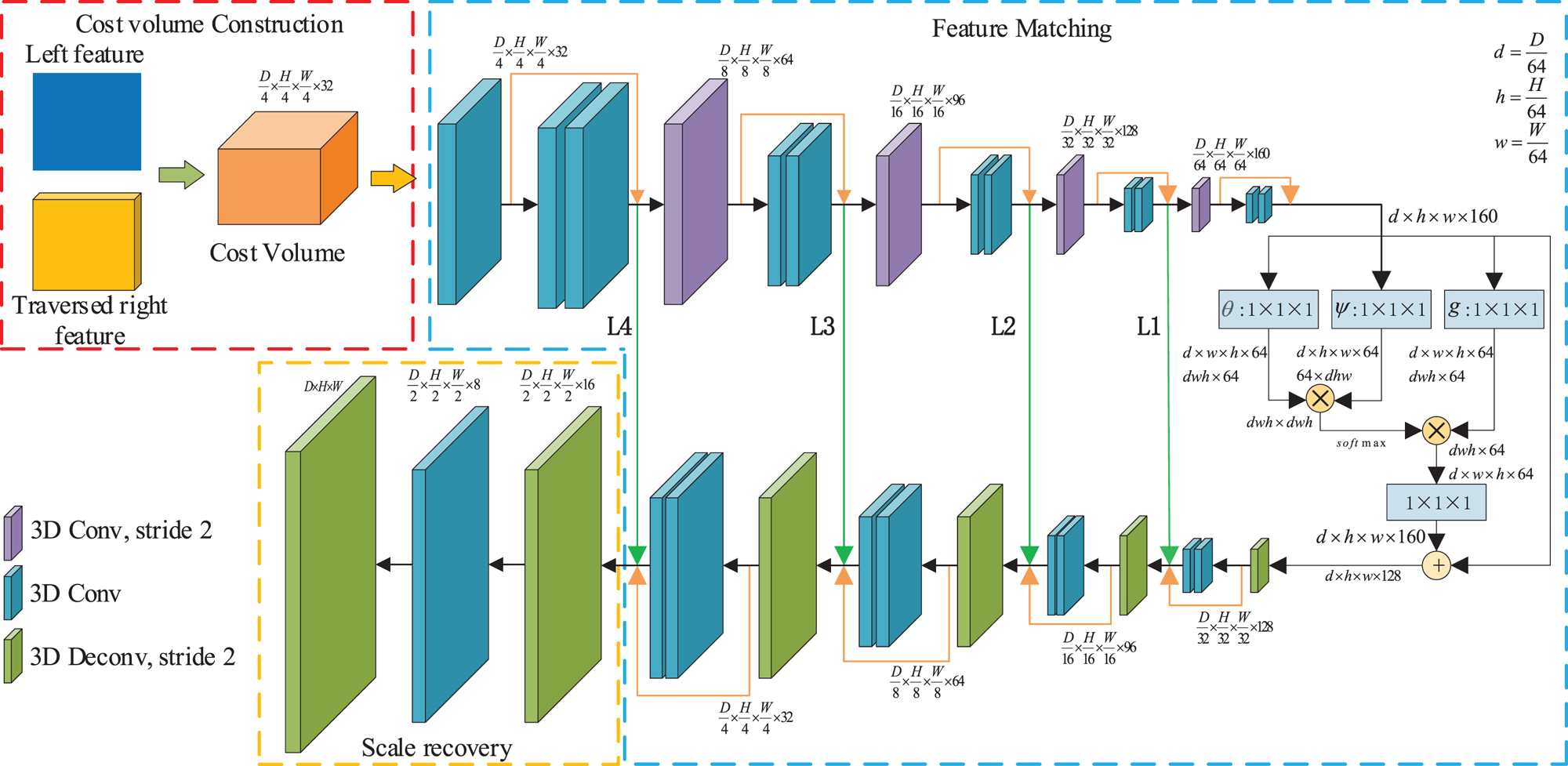
Fig. 3. The non-local attention matching module (NLAM). The NLAM module consists of feature matching part and scale recovery part. Note that the feature maps are shown as feature dimensions, e.g. $D \times H \times W \times F$ means a feature map with disparity number$D$
 , height$H$
 , width W, and feature number$F$
 . Here, $L\ast$
 denotes different scale levels of the feature maps.
In this module, we apply a series of 3D convolutional operations to obtain the matching volume, and each convolutional operation is followed by a BN layer and a ReLU layer. The NLAM module consists of feature matching part and scale recovery part.
(1) The feature matching part
The feature matching part contains $26$ convolutions with stride one or two for regularizing the variance-based cost volume. This part has four levels, and we pass the feature maps between the same level to form the residual architecture, avoiding losing the critical information. Each level consists of an up-sampling or a sub-sampling convolution, and a residual block. After the $L4$
 level, we adopt a non-local block as an attention block for further improving global matching learning.
To further understand the non-local attention mechanism, our feature matching part could be viewed as the group of the hierarchical 3D convolution block and the non-local block. The hierarchical 3D convolution block is an encoder–decoder architecture; it encodes the feature map by sub-sampling and decodes the encoded feature by up-sampling, as shown in Fig. 4.

Fig. 4. The encoder–decoder architecture. The pink block means the encoding process. The green block means the decoding process.
As shown in Fig. 4, we define the encoder and decoder process, respectively as:

where n denotes the number of the encoder and decoder, i denotes the level of the encoder or decoder, and ${{\mathcal F}_E}$ or ${{\mathcal F}_D}$
 denotes the process of each encoder or decoder.
In the encoder–decoder architecture, the worst drawback is that the convolution is a local operation. It causes the network to not further improve the receptive fields to evaluate the impact of global information on the current pixel. Thus, we use the non-local block as attention mode for promoting the understanding ability of global context, as shown in Fig. 3.
The non-local operation ${{\mathcal N}}({\cdot} )$ could be represented as:

where $x,y$ denotes the input and output, respectively, i denotes the index of an output position, j denotes the index of all possible positions, $f({\cdot} )$
 denotes the response function of global influence on current position ${x_i}$
 , $g({\cdot} )$
 denotes a representation of the input signal at the position ${x_j}$
 , and ${{\mathcal C}}({\cdot} )$
 denotes the total influence for normalizing the response.
In our non-local block, we apply the Gaussian function to compute similarity in an embedding space. We set the response function $f({\cdot} )$ as:
as:

where $\theta ({{x_i}} )= {W_\theta } \cdot {x_i}$ , $\phi ({{x_j}} )= {W_\phi } \cdot {x_j}$
 . Similarly, $g({\cdot} )$
 could be set as $g({{x_j}} )= {W_g} \cdot {x_j}$
 . Thus, the ${{\mathcal C}}({\cdot} )$
 could be set as ${{\mathcal C}}(x )= {\sum _{\forall j}}f({{x_i},{x_j}} )$
 . In this response function, the process of $(1/{{\mathcal C}}(x)){\sum _{\forall j}}f({{x_i},{x_j}} )$
 could be viewed as a softmax operation. In addition, we add y and x for a residual learning. In our architecture, the non-local block could be defined as:

After the non-local attention step, we feed the fused global feature into the decoding process as presented in equation (2) or Fig. 4. The non-local block could improve the performance of matching effectively. After this part, we could obtain the matching volume but in a low resolution $1/4H \times 1/4W \times 1/4D$ . Thus, we should recover the scale to get the final matching volume.
(2) The scale recovery part
The scale recovery part contains one convolution and two de-convolutions for recovering the size of the input image. The output of our NLAM module is a final matching volume with size $D \times H \times W$ from the variance-based cost volume.
D) Disparity map regression by soft argmin
In this step, we will estimate the initial disparity map from the matching volume. Thus, we naturally embed our matching volume into a 3D to 2D process. The simplest way to recover the initial disparity map $\hat{d}$ from the matching volume M is the pixel-wise winner-take-all such as an argmax operation. However, this way is unable to predict sub-pixel estimation and less robust [Reference Yao, Luo, Li, Fang and Quan5, Reference Kendall, Martirosyan, Dasgupta and Henry13]. Thus, we predict the disparity map by passing an argmin operation. First, we convert the matching volume M to the probability volume ${{\mathcal P}}$
 via the softmax operation $\sigma ({\cdot} )$
 . Then, we take the sum of each disparity d weighted with its probability. The soft argmin process is defined as:

where ${{\mathcal P}}(d )$ denotes the probability estimation for all pixels of the image at disparity d. ${M_d}$
 denotes all value of the $d$
 -th layer in the matching volume M.
The above method could accurately approximate the disparity d in the range from $0$ to ${D_{\max }}$
 . The output initial disparity map is the same size as the input image.
E) Disparity map refinement by geometry refinement module
The initial disparity map from the probability volume is a qualified output, but the boundaries may suffer from over-smoothing in the recovery size part of the NLAM module, or the completeness of the object suffers from the missing piece in the occlusion area. Notice that the input image contains complete boundary information, and the output of 2D GFL module contains the semantics feature, we thus use the input image and the semantics feature as guidance to refine the initial disparity map. Inspired by the recent multi-view stereo algorithm [Reference Yao, Luo, Li, Fang and Quan5], we redesign a geometry refinement (GR) module at the end of NLCA-Net, as shown in Fig. 5.

Fig. 5. Geometry refinement module (GR). The initial disparity map, the left image, and the semantics feature are fed to the GR module. After this module, we get refined disparity map. Here, blue block means the 32 convolutions with the size$3 \times 3$ , and green block means the $1$
 convolution with the size$3 \times 3$
 .
.
In the GR module, the initial disparity map, the left image, and the semantics feature are concatenated as the input. Notice that the size of the semantics feature is only quarter in width and height dimension compared to input images. Therefore, we first upsample the semantics feature, then use the $1 \times 1$ convolutional filter to adjust it. Next, we concatenate them as a $38$
 -feature input and send them to eight-layer residual network, which consists of the $32$
 convolutional filters with the size $3 \times 3$
 . After that, we apply one convolutional filter to obtain the difference, and the initial disparity map is added back to generate the refined disparity map. The last layer does not contain the BN layer and the ReLU layer. After the GR module, we could get the refined disparity map.
F) Loss function
The loss functions consider both the initial disparity map and the refined disparity map. We use the ${L_1}$ loss to evaluate the difference between the ground truth and the predicted disparity map. Due to the ground truth sparse disparity map, we only consider those pixels which are valid. The $Los{s_{{L_1}}}$
 is defined as:

where ${P_{valid}}$ denotes the set of valid ground truth pixels, ${N_1}$
 denotes the total number of valid ground truth pixels, $d(p )$
 denotes the ground truth of pixel p, ${\hat{d}_i}(p )$
 denotes the initial disparity map value of pixel p, and ${\hat{d}_r}(p )$
 denotes the refined disparity map value of pixel p.
To further improve the robustness and performance of the non-occluded area, we apply the warping loss to our loss function. The warping function is widely used in the traditional methods, and the previous learning method utilizes the warping function to structure the warping loss which gives the network self-supervised ability [Reference Zhong, Dai and Li21]. To solve the different illumination between left–right images, we introduce a structural similarity (SSIM) term $S({\cdot} )$ [Reference Wang, Bovik, Sheikh and Simoncelli37] to improve the robustness. The $Los{s_w}$
 is defined as:

where ${\textbf{n}_{valid}}$ denotes the set of pixels in the non-occluded area, ${N_2}$
 denotes the total number of valid pixels in the non-occluded area, ${I_L}$
 denotes the left image, ${I^{\prime}_L}$
 denotes the warping image which is reconstructed from the right image and the refined disparity map, and ${\lambda _1},{\lambda _2}$
 denote the balance between structural similarity and image appearance difference.
Our loss function for stereo matching is defined as:

where $\alpha$ denotes the weight of $Los{s_{{L_1}}}$
 , and $\beta$
 denotes the weight of $Los{s_w}$
 .
.
IV. EXPERIMENTS
In this section, we will evaluate the performance of our method on two widely used stereo datasets: SceneFlow and KITTI. First, we show our implementation details about the network setting and training method, as shown in Section A. Then, we compare the contribution of the different components in NLCA-Net, as shown in Section B. Finally, we quantize the performance of our method and compare it with the state-of-the-art methods on the KITTI 2012 and 2015, as shown in Section C.
A) Implementation details
In this section, we implement NLCA-Net by Tensorflow with $5.46$ M trainable parameters, and the code will be released at the Github website.Footnote 1 To obtain the final model, we should choose the hyper-parameters, train, and evaluate the model.
(1) Hyper-parameters and datasets
For the hyper-parameters in this network, we set the max disparity $D = 192$ to ensure all possible disparity values in the image could be detected. In the loss function, we initially apply ${\lambda _1} = 0$
 , ${\lambda _2} = 0$
 , $\alpha = 1$
 , and $\beta = 0$
 and then empirically test the best parameters based on our experiments.
For the datasets, we will train and evaluate our approach on these stereo datasets as follows:
• SceneFlow: a large synthetic dataset consists of $35454$
 training and $4370$ testing images with the size $H \times W = 540 \times 960$, which provides dense and clear disparity maps as ground truth. It could help us to adequately assess the performance of different model variants without worrying about over-fitting, and to make the pre-trained model have better generalization performance.
• KITTI 2012: a challenging and varied road scene dataset contains $194$
training and $195$ testing images with the size $H \times W = 376 \times 1236$, which only provides sparse disparity maps as ground truth for training images.• KITTI 2015: a real-world street views dataset contains $200$
training and $200$ testing images with the size $H \times W = 374 \times 1236$, which only provides sparse disparity maps as ground truth for training images.


(2) Training method
For the training process, our network can be trained from random initialization in an end-to-end way with the supervision of stereo pairs and optimized using Adam Optimizer with ${\beta _1} = 0.9$ , ${\beta _2} = 0.999$
 , and a batch size of $1$
 for each GPUs. Before training, we normalize stereo pairs with pixel intensities level ranging from $0$
 to$1$
to$1$ , and randomly crop them into $256 \times 512$
 . During the training process, we adopt the multi-step training method with four Nvidia 1080Ti GPUs. Thus, the training process consists of two parts: the pre-training process and the fine-tuning process.
• In the pre-training process on the SceneFlow dataset, the learning rate is initially set to $1 \times {10^{ - 3}}$
for $30$ epochs and obtains the pre-train model.• In the fine-tuning process on the KITTI dataset, the learning rate is set to $1 \times {10^{ - 3}}$
for $800$ epochs and then reduced to $1 \times {10^{ - 4}}$ for the other $100$ epochs. After the training process, we get the final model.


(3) Evaluating metric
For evaluating our model and comparing with the state-of-the-art methods published recently, we show our results' errors with the following metrics, which have been widely used in the website of KITTI dataset:

where d denotes the ground truth of disparity, $\hat{d}$ denotes the estimated depth, m denotes the threshold of error pixel, $[{\cdot} ]$
 denotes the Iverson bracket, $bg$
 represents the set of all points in background regions of the images, $fg$
 represents the set of all points in foreground regions of the images, and T represents the set of all points in the images.
B) Ablation study for NLCA-Net
To verify our design's effectiveness, we conduct experiments with different settings to evaluate NLCA-Net on the SceneFlow dataset. We train different model variants like the pre-training process, as presented in Section A. We first compare the performance of different settings, including the 2D GFL module, VBCM, the NLAM module, and the GR module, as shown in Table 1. Then, we present the representative results of our model and ablation study of loss weight, as shown in Fig. 6 and Table 2. Moreover, we test the impact of the different numbers of the non-local on the model, as shown in Table 3.
Table 1. Evaluation of NLCA-Net with different settings.

Computed the percentage of three-pixel-error on the SceneFlow and KITTI 2015 test set.

Fig. 6. SceneFlow test data qualitative results. From left: left stereo input image, ground-truth, disparity prediction.
Table 2. Influence of weight values for ${\lambda _1}$ , ${\lambda _2}$
 , $\alpha$
 , and $\beta$
 on three-pixel-error.

We empirically found that 0.85/0.15/0.8/0.2 yielded the best performance on the SceneFlow test set.
Table 3. Influence of the different numbers of the non-local blocks on the model.

Here R denotes the number of the non-local blocks.
As shown in Fig. 6 and Table 1, it qualitatively demonstrates the benefits of using the modules which we proposed. First, the 2D GFL and NLAM modules show a significant performance improvement for the matching accuracy. For the GFL module, it enhances the scene understanding ability of the model effectively; for the NLAM module, it has a strong regularization ability to learning the matching rules and can facilitate the learning process. Second, the GR module and $Los{s_w}$ function improve the matching accuracy a little. On a good baseline, the GR module could further improve the performance and $Los{s_w}$
 function could achieve $1\%$
 improvement on whole pixels and $4\%$
 on non-occluded pixels. Finally, the VBCM provides better testing accuracy compared with traditional concatenation way, and it saves half-memory of the cost volume, which reduces about 300 M running memory of the whole framework.
As shown in Table 2, we conduct experiments with various combinations of loss weights which have the relationship about ${\lambda _1} + {\lambda _2} = 1$ and $\alpha + \beta = 1$
 . For the baseline, we only use the ${L_1}$
 loss function and then continuously adjust the loss weights to find the weights which yield the best performance. The result shows that the weight settings of $0.85$
 for ${\lambda _1}$
 , $0.15$
 for ${\lambda _2}$
 , 0.8 for $\alpha$
 , and 0.2 for $\beta$
 obtain the best performance, which is a $2.87\%$
 three-pixel-error rate on the SceneFlow test set and a $1.96\%$
 three-pixel-error rate on the KITTI test set.
Finally, we also test our model with different non-local block (NL-block) numbers. In this part, we set a model without NL-block as the baseline. The impact of NL-block is tested by increasing the NL-block number in the model. As shown in Table 3, we list the results with different NL-blocks on the SceneFlow and KITTI 2015, indicating that performance can be improved by introducing NL-block into the model. It is also noticed that the improvement decays gradually as the number of NLB increases, showing the boundary effect.
C) KITTI 2012 and 2015 benchmark results
To evaluate the performance of our model, we compare the performance of NLCA-Net with other state-of-the-art methods on the KITTI dataset. We use the multi-step training method to train the model, as shown in Section A. We present the representative images of our model and other state-of-the-art methods, as shown in Figs 7 and 8. Then, we evaluate the performance of our model on the KITTI website,Footnote 2 as shown in Tables 4 and 5. Besides, we compare our model with other competing algorithms in the reflective regions, as presented in Table 6.

Fig. 7. KITTI 2012 test data qualitative results. We compare our approach with state-of-the-art methods (HD3-S and GwcNet), and we highlight our advantage in the error maps. Note that, in the error maps, the deeper red pixels mean higher error rate in the occluded regions and white pixels denote ≥5 pixels error in the non-occluded regions.

Fig. 8. KITTI 2015 test data qualitative results. From left: left stereo input image, disparity prediction, error map. Note that, in the error maps, depicting correct estimates (<3 px or <5% error) in blue and wrong estimates in red color tones.
Table 4. Results on KITTI 2012 stereo benchmark.

Average end-point-error (EPE) and the percentage of different pixel-error are used for evaluations on the KITTI 2012 test set. Compared with other algorithms, our approach achieves the best performance in most cases.
* The number of the non-local blocks is 3.
Table 5. Results on KITTI 2015 stereo benchmark.

Our approach achieves comparable performance to state-of-the-art methods.
* The number of the non-local blocks is 3.
Table 6. Comparisons of different state-of-the-art methods in the reflective regions.

Average end-point-error (EPE) and the percentage of different pixel-error are used for evaluations on the KITTI 2012 test set. Compared with other algorithms, our approach achieves the best performance in most cases.
* The number of the non-local blocks is 3.
As shown in Figs 7 and 8, the proposed method could produce dense and clear disparity maps. For the non-occluded region, the proposed method shows the powerful performance; the disparity maps predicted by NLCA-Net are sharper and more complete than other learning methods. Even if in the occluded region, the proposed method still provides high-level performance and significantly outperforms other state-of-the-art methods, as shown in Fig. 9. The results show that our method can notably reduce the error rate on the occluded area and handle well with the large textureless regions. It also means the semantic information plays an important role, which offers the boundary information to perfect the edge pixels of objects. Overall, the proposed method shows the incredible expressiveness in the matching task.

Fig. 9. Part zoom-up of the error maps on the occluded region. From left: original image, HD3-Stereo, GwcNet, and ours. The result shows that our method can notably reduce the error rate on the occluded area and handle well with the large textureless regions.
As shown in Tables 4 and 5, it qualitatively demonstrates the performance of the proposed method. Compared with other methods, the proposed method yields more precise and robust disparity maps, particularly in the non-occluded regions. For the KITTI 2012 dataset, our approach is very close to HD3-Stereo [Reference Yin, Darrell and Yu22] on non-occluded (Out-Noc) in the error rate of 2 pixels; but for other quality indexes, our method all achieves the best performance as shown in the table. For the KITTI 2015 dataset, our approach shows comparable performance and markedly outperforms other competing algorithms, including the previous best result (HD3-Stereo [Reference Yin, Darrell and Yu22] and GwcNet [Reference Guo, Yang, Yang, Wang and Li18]). In short, the proposed approach is superior to state-of-the-art methods in most cases.
As shown in Table 6, it qualitatively shows the advantage of our model in the reflective regions. In our designs, we use attention mechanisms and semantic information to enhance the ability of scene understanding. Thus, in the reflective region, the proposed method achieves the best performance of all quality indexes and significantly outperforms other state-of-the-art methods. It indicates the effectiveness of our matching network based on the contextual attention mechanism, which exhibits robustness to the reflective regions.
V. CONCLUSIONS
In this work, we present a highly efficient network architecture for stereo matching. The proposed model can exploit the global context information to achieve superior performance in the matching task. The NLAM significantly enhances the ability of scene understanding to improve the accuracy in the challenging regions, such as occlusions and large textureless/reflective areas. The variance-based cost volume can provide the similarity information and reduces some memory, thus further improving the performance. The experiment shows that the proposed method can improve the performance in challenging regions and outperform state-of-the-art methods in most cases. For future work, we are interested in exploring the generative adversarial network's potential to achieve higher accurate semi-supervised or unsupervised stereo matching.
Acknowledgement
This work was supported in part by the Natural Science Foundation of China (61671387, 61420106007 and 61871325). The authors would like to thank the Editor-in-Chief, associate editor and the anonymous reviewers for their valuable comments and suggestions that helped improve the quality of this paper.
APPENDIX A
Detailed network structure. The core architecture of our NLCA-Net contains three modules: (1) geometry feature learning module (GFL); (2) non-local attention matching module (NLAM); (3) geometry refinement module (GR). We illustrate the detailed structure of our method is presented in Table 7. Each 2D or 3D convolutional layer contains three steps: convolution, batch normalization (BN), and ReLU non-linearity (unless otherwise specified).
Table 7. The summary of our non-local context attention network, NLCA-Net.

Zhibo Rao received his M.S. degree in electronic information engineering from Nanchang Hangkong University in 2017. He is currently a Ph.D. student in the School of Electronics and Information, Northwestern Polytechnical University, Xi'an, China. His research interests are pattern recognition, image processing, and deep learning. He has published some papers on the ICIP, APSIPA, 3DV, ICIEA, etc.
Mingyi He received his B.Eng. and M.S. degrees in electronic engineering and signal processing from Northwestern Polytechnical University (NPU), Xian, China, in 1982 and 1985, respectively, and the Ph.D. degree in signal and information processing from Xidian University, Xian, China, in 1994. Since 1985, he has been with the School of Electronics and Information, NPU, where he has been a full professor since 1996. He is the Founder and Director of Shaanxi Key Laboratory (2003–2019) and International Research Center (2016–) for Information Acquisition and Processing, and the Director and Chief Scientist of the Center for Earth Observation Research (2011–), NPU. He had been a visiting scholar at Adelaide University, Adelaide, SA, Australia, and visiting professor at Sydney University, Sydney, NSW, Australia, and Adelaide University. His research interests are advanced machine vision and intelligent processing, including signal and image processing, computer vision, hyperspectral remote sensing, 3D information acquisition and processing, neural network, and deep learning. Dr. Mingyi He is a recipient of 11 national and provincial scientific prizes and two teaching achievement prizes in China. He won the Best Paper Award in IEEE CVPR 2012, the Best Deep/Machine Learning Paper Prize at APSIPA ASC 2017, the 2017 DICTA Best Student Paper Award (as supervisor and coauthor), etc. He was also a recipient of the government lifelong subsidy from the State Council of China in 1993 and the Baosteel Outstanding Teacher Award in 2017. He received awards or certificates of honor from IEEE Signal Processing Society in 2014, APSIPA in 2019, Chinese Institute of Electronics in 2019 and 2020. He has acted as a General Chair or TPC (Co)Chair, and Area Chair for dozens of national and international conferences. He has been a member of the Advisory Committee of National Council for Higher Education on Electronics and Information in China, a member of Chinese Lunar Exploration Expert Group, the Vice-President of Shaanxi Institute of Electronics (SIP committee chair), and the Vice-Director of the Spectral Imaging Earth Observation Committee of China Committee of International Society of Digital Earth. He is an Associate Editor for the IEEE Transactions on Geoscience and Remote Sensing and APSIPA Transactions on Signal and Information Processing, a Guest Editor for the IEEE Journal of Selected Topics in Applied Earth Observation and Remote Sensing. Dr. He is a senior member of IEEE and a member of IEEE GRSS Image and Data Fusion Technical Committee, Chair of SIPTM (Signal and Information Processing Theory and Methods) Committee and BoG member of the Asia-Pacific Signal and Information Processing Association (APSIPA).
Yuchao Dai is currently a Professor with the School of Electronics and Information at the Northwestern Polytechnical University (NPU). He received the B.E. degree, M.E degree, and Ph.D. degree all in signal and information processing from Northwestern Polytechnical University, Xian, China, in 2005, 2008, and 2012, respectively. He was an ARC DECRA Fellow with the Research School of Engineering at the Australian National University, Canberra, Australia from 2014 to 2017 and a Research Fellow with the Research School of Computer Science at the Australian National University, Canberra, Australia from 2012 to 2014. His research interests include structure from motion, multi-view geometry, low-level computer vision, deep learning, compressive sensing, and optimization. He won the Best Paper Award in IEEE CVPR 2012, the DSTO Best Fundamental Contribution to Image Processing Paper Prize at DICTA 2014, the Best Algorithm Prize in NRSFM Challenge at CVPR 2017, the Best Student Paper Prize at DICTA 2017, and the Best Deep/Machine Learning Paper Prize at APSIPA ASC 2017.
Zhidong Zhu is currently a master student in the School of Electronics and Information, Northwestern Polytechnical University, Xi'an, China.
Bo Li is currently a research associate in the School of Electronics and Information, Northwestern Polytechnical University (NPU), China. He received his B.E. degree and Ph.D. degree from NPU in 2011 and 2018, respectively. During 2013–2015, he was a visiting student at the University of Adelaide, Australia. His research interests mainly focus on the deep learning and computer vision. He has published more than 10 papers in the CVPR, PR, TMM, TGRS, etc.
Renjie He received the B.E. degree in automation from Xi'an Jiaotong University in 2008, and M.E. degree and Ph.D. degree in signal and information processing from Northwestern Polytechnical University in 2011 and 2017, respectively. During 2011–2013, He was a visiting student at the University of Sydney, Australia. During 2017–2020, He has been a Research Fellow at Nanyang Technological University, Singapore. His research interests include image enhancement, restoration, visual perception, and remote sensing image analysis. He won the Best Paper Award in IEEE ICIEA 2019.


 Open access