Introduction
Filchner,Ronne Ice Shelf is one of the largest ice shelves in the world (Figure 1), It covers an area of around 500000 km2about the same as the Ross Ice Shelf, but has a higher average thickness and thus a greater volume. The ice shelf influences global climate in two ways. First, melting of ice from the base of the ice shelf is a significant component of the Antarctic mass budget and the resulting modification of the sea water plays an important role in driving deep convection in the Southern Ocean, where about 80% of Antarctic Bottom Water is produced in the Weddell Sea region (Reference JenkinsJenkins, in press). Secondly, fast-flowing ice streams draining the Antarctic ice sheet disgorge into the ice shelf. Where the inland ice sheet is grounded below sea level, as in most of West Antarctica, one of the major problems is to understand the stabilizing role of the ice streams and the way this is influenced by the ice shelf. Accurate surface elevations reveal ice-shelf structures related to melting and freezing beneath it and are needed for numerical modelling studies of the ice dynamics.
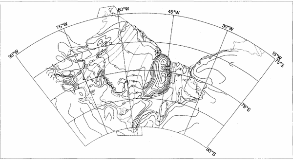
Fig. 1. Map sheet lines indicating the area covered by the Topographic Map (Satellite Image Map) 1:2000000 Filchner,Ronne Ice Shelf.
The Filchner,Ronne Ice Shelf Programme (FRISP), formed in 1984 as a sub-group of the SCAR Working Group on Glaciology, co-ordinates glaciological activities of countries working in the region. Since the International Geophysical Year (IGY), 1957–58, significant work has been carried out by Argentina, Germany, Scandinavian countries, the U.K., the U.S.A. and the former U.S.S.R. As a result of a collaborative project between institutes in Germany, the U.K. and Russia, the Institut für Ange-wandte Geodäsie (IFAG), Frankfurt am Main, has published a topographic map (1993) (a copy is enclosed in the end pocket of this volume) of the whole region including the catchment area using the most recent surface-elevation values from ground and airborne campaigns. A mosaic of Landsat images has been used as background, complementing a glaciological feature map produced by an earlier collaborative exercise (Reference Swichinbank, Brunk and SieversSwithinbank and others, 1988). Surface elevations derived from radar-altimeter data from the ERS-1 satellite fast-delivery product set over the ice shelf itself have been contoured to compare with the topographic map (1993).
A basic problem in producing a surface-elevation map for the ice shelf is that there are thick layers of marine ice (Reference OerterOerter and others, 1992) beneath large parts of it which are sufficiently absorbent to prevent the total ice thickness being sounded by radar methods (Reference Crabtree and DoakeCrabtree and Doake, 1986; Reference ThyssenThyssen, 1988). There could also be a mushy layer at the interface between the ocean and the ice-shelf base (Reference Nicholls, Makinson and RobinsonNicholls and others, 1991)which prevents seismic techniques from obtaining a distinct reflecting horizon. Thus, elevations cannot always be obtained by inverting ice thicknesses assuming hydrostatic equilibrium. Instead, elevations have to be derived using other techniques such as trigonometric or barometric levelling.
Topographic map (satellite-image map) 1:2 000 000 Filchner,Ronne ice shelf
Satellite imagery
To map the whole region of the Filchner,Ronne Ice Shelf as well as the contiguous catchment area, a digital mosaic of satellite imagery has been constructed to cartographic quality. The mosaic has been assembled from 65 Landsat -4 and -5 Multispectral Scanner (MSS) scenes acquired between January 1985 and March 1988, four Landsat -1 and -2 MSS scenes acquired between October 1973 and February 1974, and NOAA AVHRR data acquired between 1980 and 1987 of areas not covered or not scanned cloud-free by the Landsat satellite.
Digital geometric construction of this mosaic is based on measurements of satellite-image coordinates of topographic features appearing in more than one Landsat scene. About 500 of these identical points ("tie points"), for which ground coordinates arc not known, have been used (Reference Sievers, Grindel and MeierSievers and others, 1989). For referencing the image mosaic to the geographic map coordinate system, 28 ground-control points were available, positioned either by GPS or Doppler-satellite techniques. The standard deviation of coordinates of ground control and tie points is estimated to be ±125m in x and y positions. At the margins of the mosaic, especially at. the southern boundary of the Filchner,Ronne Ice Shelf, the deviations are probably larger due to lack of ground control in this area.
Solar radiation reflected from the terrain surface is recorded by the MSS sensor in four spectral bands of the visible and near-infrared spectrum. Figure 2 shows that various types of snow and ice are equally discernible in all four MSS bands. This means that all relevant topo-graphic-glaciologic information is contained in only one band. Band 3 was chosen for reproduction of the mosaic because of its greater evenness in the data recording of all images used (peak of frequency and dynamic range of recorded reflected radiation). To handle the huge amount of digital data in the mosaic, the original pixel size (60 m by 60 m) had to be increased to a size of 240 m by 240 m
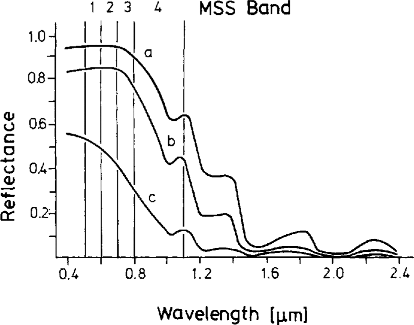
Fig.2. Spectral reflectance of (a) dry new snow, (b) old snow and (c) blue ice after (Reference Rott and Arnberger Rott, 1989)
Topographic-glaciologic data
To aid map users in the inerpretation of the satellite-image mosaic, a selected number of topographic-glaciologic features were cartographically represented on the image map and arc shown in Figure 3 These are: the ice front as the seaward cliff of the ice shelf; the ice wall as the seaward cliff of the inland ice sheet or of the ice cap of an ice rise; the grounding line as the boundary between floating and grounded ice of the inland ice sheet or an ice rise, which on the topographic map (1993) is distinguished from the grounding line of ice rumples; the margins of glaciers or ice streams. Classification of the features was conducted by eye according to criteria developed byReference Heidrich, Sievers, Schenke and ThielHeidrich and others (1992) on geo-referenced satellite imagery enlarged to a 1:400 000 scale. Digitization was carried out using a Geographic Information System. The number of features shown has been limited in order not to obscure details of the mosaic.

Fig.3. TopograPhic features and suiface-elevation contour lines as shown on the topographic map (1993).
Airborne and terrestrial elevation data
Most of the elevation data used in the topographic map (1993), and shown in Figure 3, were previously unpublished. The most recent data available for a given area were selected for compilation, resulting in seven zones. The final data set was matched at the zone boundaries, contoured automatically and then smoothed by hand to reflect the morphology of the ice surface as revealed in the satellite imagery.
Surface-elevation data from airborne and ground measurements have been integrated from a number of sources. Airborne radar and barometric data collected by the scientific consortium Sevmorgeologija (of the former Ministry of Geology of the U.S.S.R.), Sankt Peterburg, Russia, since 1976 were used as the base. Similar, but more recent, data from the Westfälische Wilhelms-Universität, Mänster, Germany (Reference Thyssen, Bombosch and SaudhägerThyssen and others, 1992), and the British Antarctic Survey, Cambridge, England, were used in specific areas, particularly over the Ronne Ice Shelf. Where an unambiguous ice thickness was obtained, the elevations have been calculated by assuming hydrostatic equilibrium. The most difficult area in which to determine accurate elevations was the central part where there is the largest amount of basal ice accumulation. Only barometric measurements could be used, tied to trigonometric levelling where possible, and inconsistencies removed by a cross-over analysis. The determination of accuracies is described on the map. They vary from ± 2 to ± 7 m on the ice shelf. Oversnow trigonometric levelling by the Technische Universität Braunschweig, Germany, in the northeastern part of the ice shelf, tied to sea level at the ice front, has given accuracies of ± 1 m. Accuracies reduce to about ± 20 m in, the grounded-ice areas where elevations have been derived from barometric measurements made mainly during airborne surveys by the British Antarctic Survey, Cambridge, England; U.S. National Science Foundation, Washington, DC, U.S.A.; and Sevmorgeologija, Sankt Peterburg, Russia.
Radar-altimeter data
Ellipsoidal heights (elevations above ellipsoid)
The ERS-l radar-altimeter data were taken from the fast-delivery products (ERSl.ALT.FDC) distributed by the European Space Agency (ESA), These products are processed directly by the ESA ground stations on reception of altimeter-telemetered data. They provide 1 Hz estimates of the fundamental parameters, ing satellite to ground range, at an along-track ground spacing of 6.7 km. The FDC products were post-processed at the Mullard Space Science Laboratory (MSSL), England, to retrieve the best possible reference data set of ellipsoidal heights (i.e. height of data points above ellipsoid; Reference Frei, Graf, Meier and SchreierFrei and others, 1993). First, the bad data points were filtered out using a “pulse peakiness” criterion developed by Reference Strawbridge and LaxonStrawbridge and Laxon (in press). The FDC parameter list includes a pulse-peakiness parameter, which describes the shape of the average of 20 altimeter wave forms, from which the elevation data given in the products are derived, The range data are taken from the on-board estimate, which is optimized for return-echo wave forms characteristic of ocean surfaces. It is assumed that, if the pulse-peakiness parameter exceeds a value of I, the on-board estimate is unreliable and hence the data point is discarded. The FDC data are distributed with the ERS-l “restituted” orbit; we have replaced this with the more accurate “preliminary” orbit. Although atmospheric corrections are given in the products, they are rough estimates and of little value in the geographic area under consideration. No attempt was made to include a tidal correction. No slope correction was applied, as we are only interested here in the effectively flat ice shelf. In order to reduce the effects of weather, a single 35 d repeat data set was used, (cycle-93) from early 1993. Data points used from this cycle are shown in Figure 4 A bulk-quality assessment of the data set was carried out by applying a cross-over analysis technique similar to that described by Reference TaiTai (1989). The residuals arc of the order ± 1m in the central area of the ice shelf, although they are higher around the grounding lines. A further increase in accuracy can only be achieved through analysis of the wave-form data set. The data set was interpolated using a bilinear method on to a 5 km x 5 km grid, with a search radius of 7.5 km and a small along-track overlap, prior to conversion to orthometric height (elevation above sea level; Reference Frei, Graf, Meier and SchreierFrei and others, 1993).

Fig.4. Generalized geometry for photoclinometrx Definitions of the angles are given in the text.
Reductions to geoid
Heights derived from radar altimetry must be converted to orthometric heights to be comparable with surface elevations on the topographic map(1993). The Conver-sion was carried out using the Geodetic Reference System 1980, GRS80 (Reference MoritzMoritz, 1984), which has geometric para-meters that are virtually identical to those of the WGS84 ellipsoid.
Ellipsoidal heightsH are related to orthometric heightsh for a given geoid N by
The geoid of the geopotential model (GPM) OSU9lA (Reference Rapp, Wang and PavlisRapp and others, 1991) was used for the reduction of the ellipsoidal heights. The OSU9lA model is a spherical harmonic expansion of order 360 and thus resolves structures with wavelengths greater than 100 km. Presently, it is the best available solution of a global GPM for the Antarctic region. The error of absolute geoidal heights in relation to the mean Earth ellipsoid is about ±0.5m. The accuracy depends on the data introduced into the solution and thus is expected to be lower in the Antarctic regions.
The orthometric heights h calculated according to (Equation 1)have still to be shifted to sea level. The shift is to allow for two a priori unknown corrections: the difference between the geoid and the stationary sea-surface topography and for the difference between the mean Earth ellipsoid and GRS80 Reference Frei, Graf, Meier and Schreier(Frei and others, 1993). For determination of the shift parameter, comparisons with trignometrically levelled elevations on the Ronne Ice Shelf were used. From the comparisons, we obtained a difference of ±2.0m between the geoid and mean sea level of the Weddell Sea, so that the final relation for orthometric height h' is:
The final results are shown in Figure 5 Our best estimate of the possible error of the elevations derived from the radar-altimeter data is ±5 m.
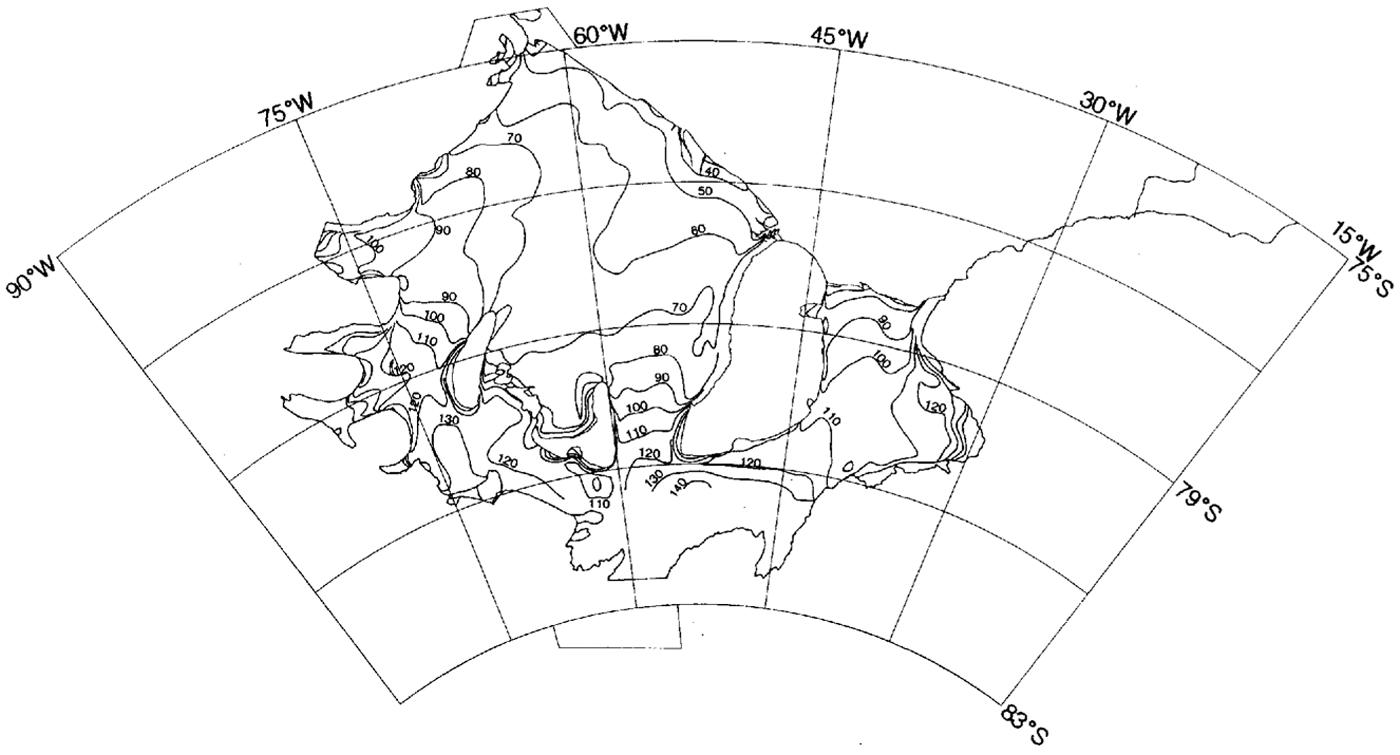
Fig.5. Contoured orthometric elevation(m) of Filchner,Ronne Ice Shelf derived from ERS-1 radar-altimeter data and geopotential model OSU91A (Reference Rapp, Wang and PavlisRapp and others, 1991).
Comparison of results
The overall comparison between the topographic map(1993) and the radar-altimeter data is within the indicated standard deviations, especially in areas where little marine ice has accumulated at the ice-shelf base. For example, the 50 m contour near the ice front on the Ronne Ice Shelf is similar in both cases. However, there are significant detailed differences in some areas, sometimes attributable to the different scales on which the data have been collected but sometimes reflecting the difficulty in obtaining accurate elevations from barometric heighting.
When compiling the topographic map (1993), in areas where we had competing data sets we chose the most recent set. In the case of the centre of the Ronne Ice Shelf, it meant that data processed by the Münster group were used in preference to data processed by Sevmorgeologija. There is perhaps a better correlation between the Sevmorgeologija data and the radar-altimeter data but the flatness of the area amplifies errors in elevation and could move contour positions substantially.
The 70 m contour illustrates the differences between the topographic map (1993) and radar-altimeter data well. There is agreement to within the quoted standard deviations from Berkner Island to 57° W and from 60° W to the Antarctic Peninsula. Between 57° and 60° W, the radar-altimeter data show a disturbed zone in a trough running back from the ice front towards Korff Ice Rise, although a case could be made for drawing the 70m contour in the position shown on the topographic map(l993). The overall trend from the radar data of a depressed central area is reminiscent of the meteoric ice-thickness distribution (Reference Crabtree and DoakeCrabtree and Doake, 1986).
Downstream of Evans Ice Stream, the topographic map(1993) shows a number of closed elevation loops which do not appear in the radar-altimeter data. These loops are located in an area with a narrow trough of basal marine ice and may be due to errors arising from the more complicated processing of barometric data from flights from several different seasons.
In most other areas, such as behind Korff and Henry Ice Rises on Ronne Ice Shelf and over Filchner lce Shelf, there is an excellent agreement at the level of accuracy quoted for the topographic map(1993) and the radar-altimeter data.
5 Conclusions
At the 5 m level of accuracy, the contour lines on the published topographic map (1993) are equivalent to the ERS-I fast-delivery radar-altimeter-derived elevations. To improve the topographic map (1993) of derived elevations significantly, we require an order of magnitude better source of consistent data. This is most likely to be provided by ERS-l radar altimetry once corrections for orbits, tides, ionosphere, atmosphere, surface, etc. are made. One source of error that will remain difficult to quantify is the geoid reduction. The geoid gets worse away from the coast and for improvement requires a campaign of gravity measurements.
Acknowledgements
We should like to thank Dr P. Challenor (James Rennell Centre, Southampton) and Dr F. Strawbridge (MSSL) for implementation of the Tai cross-over analysis algorithm.