


The Isotope Paleothermometer
Isotopic ratios of precipitation in the polar regions reflect the temperature difference between the moisture source and the vapor from which snow forms. If the temperature at the moisture source is constant, or if variable source temperature effects can be accounted for (e.g. Reference Cuffey and VimeuxCuffey and Vimeux, 2001, and references therein; Kavanaugh and Cuffey, 2002), then variations in stable-isotope ratios in polar snow reflect variations in the temperature at which the precipitation formed. Over the Antarctic ice sheet, the atmosphere generally has a temperature inversion, caused by longwave radiative cooling at the snow surface. Since precipitation in the Antarctic forms just above the inversion layer (Reference RobinRobin,1977), stable-isotope ratios in new snow reflect the relatively warm temperature above the inversion layer, rather than the relatively cool surface temperature. Reference Jouzel and MerlivatJouzel and Merlivat (1984) showed that a linear relationship (r2 = 0.98) exists between surface temperatures and inversion temperatures, based on measurements over the whole Antarctic continent. Over very cold areas, such as Vostok, the temperature difference is approximately 20˚C. Because of these known controlling processes, the stable-isotope ratios in snow can be related to the air temperature at the site of deposition (e.g. Reference JouzelJouzel and others, 1997). However, if some processes operate effectively only under certain climate conditions, then they may not be reflected in the isotope calibration.
Stable isotopes in ice cores work well as a proxy for the temperature at the inversion layer at the time of snow formation where net accumulation rate is relatively high, such that snow is buried quickly. However, in low-accumulation areas, snow can remain near the surface for several years. During this time, the snow is exposed to ventilation and vapor exchange with the atmosphere. We explore the possibility that this snow may lose its original isotopic signature by equilibrating with water vapor in the boundary layer over the ice-cap surface.
Stable-isotope concentrations of vapor in the near-surface boundarylayer are clearly related to climate, and are observed to vary in a fashion similar to cloud temperatures. Therefore, equilibrationbetween atmospheric vapor and snow would not invalidate stable isotopes as a climate proxy. However, it would indicate a need to further assess the calibration coefficient between isotopes and temperature. Ways in which equilibration could bias the isotopic record include: (a) snow precipitated in one season (e.g. winter) may equilibrate with the atmosphere in a different season (summer), and (b) the extent to which equilibration occurs may differ under different climate regimes. the latter point may have important implications for the comparison of climate changes recorded in cores from low-accumulation-rate sites such as Vostok with those observed in central Greenland.
Snow–Atmosphere Isotopic Exchange
An established body of literature on post-depositional movement of stable isotopes in polar firn (Reference JohnsenJohnsen, 1977; Reference Whillans and GrootesWhillans and Grootes, 1985; Reference Cuffey and SteigCuffey and Steig, 1998; Reference Johnsen, Clausen, Cuffey, Hoffmann, Schwander, Creyts and HondohJohnsen and others, 2000) addresses primarily the decay of seasonal cycles by diffusion, as isotopes are locally redistributed within the firn during the long time between deposition and pore close-off. During this redistribution, the firn remains a closed system. Although we use similar concepts to describe isotope movement in snow, we address a different question: are stable isotopes part of an open system for a limited time after deposition, such that the mean isotopic ratio of snow can change?
Changes in isotopic content of snow have been observed in temperate environments. Reference Moser and StichlerMoser and Stichler (1975) measured the isotopic composition of surface snow as a function of time, in Switzerland. They found that the deuterium δD changed by several per mil daily; they attributed this to vigorous mass transfer between the snow and the atmosphere as a result of daily heating and cooling at the snow surface. the changes in bulk δD of the snow resulted primarily from the addition or subsequent loss of atmospheric water, with a different isotopic ratio.
In contrast, we do not expect that the isotopic composition of surface snow changes measurably on a daily cycle in the polar regions. Compared with the temperate area studied by Reference Moser and StichlerMoser and Stichler (1975), there is a much smaller reservoir of vapor in the atmosphere in the polar regions, owing to the exponential relationship between temperature and saturation vapor pressure. the isotopic composition of surface snow in polar regions may evolve toward equilibrium with the overlying air mass, but it will do so on a much longer time-scale, and possibly by different processes. Consequently, in the polar regions, we must consider not only time-scales for direct mass transfer between the snow grains and the atmospheric vapor phase, but also the time-scales for isotopic diffusion within the ice grains and through the permeable snow. for polar snow to equilibrate with vapor in the atmosphere, water molecules in the snow must exchange with water molecules in the atmosphere. to exchange, they must diffuse out of their solid ice grains, then move out of the snow as vapor through the interconnected pore spaces in the firn, by diffusion or by forced ventilation. Cold temperatures impede diffusion; low wind speed and smooth microtopography impede forced ventilation; and high accumulation rate limits the time available for isotopic exchange before snow is buried too deeply to interact effectively with the atmosphere.
The direction and the amount that firn will change, isotopically, as it evolves toward equilibrium with atmospheric water vapor, depends on the isotopic value of that vapor. In perfectly still air, at some short distance above the firn, we may expect vapor saturation to be reached, in which case the vapor will be in isotopic equilibrium with average surface snow. Measurements of δ18O and δD in air samples collected at Summit, Greenland, during the summer months (Reference Grootes and StuiverGrootes and Stuiver, 1997; E.J. Steig, unpublished data) indicate that, for 12 hour averages, this situation is approximated in the first few decimeters above the surface. the isotopic composition of the vapor variesby a few per mil (δ18O) with the daily cycle, but does not appear to vary on a day-to-day basis. More than a few meters above the surface, vapor isotopic values follow that same daily cycle, but also change by as much as 10 per mil from day to day. At this site, a diurnal cycle of surface firn sublimation and fog redeposition is commonly observed (e.g. Reference Bergin, Jaffrezo, Davidson, Caldow and DibbBergin and others, 1994). the most straightforward explanation of the observed diurnal isotopic variationof atmospheric vapor is that it reflects this sublimation cycle, with the heavier isotopes preferentially removed during fog formation. the additional day-to-day variability in the air further from the surface would then reflect the mixing of local vapor from the firn with ``new’’ vapor brought by incoming air masses. for our measurements from July 2000 at Summit, this new vapor was isotopically heavier than the ambient, near-surface air (which is in equilibrium with older snow that may have fallen in spring, rather than summer). to the extent that isotopic re-equilibration with this airmass could occur, it would lead to enrichment of the firn.
Characteristic Times for Isotopic Change
To fully interpret the stable-isotope records in ice cores, a verifiable process-based transient model of the complete system of snow, pore vapor and atmospheric vapor will be needed. Without modeling those physical processes, we cannot predict the exact amount of modification of δ18O of surface snow that fully or partially equilibrates with vapor in the near-surface atmosphere. Current uncertainty in the value of the atmospheric isotopic ``target’’, toward which equilibration would proceed, suggests that it may be premature to use such a sophisticated model. However, as an initial step, we can assess whether snow in a particular environment should be assumed to have been modified or not. We do this, not by modeling changes in stable isotopes in snow, but rather by calculating the characteristic time required for the snow to change. We do not specify or determine at this preliminary stage just how large those changes might be. By restricting this initial exploration to the response times, rather than the changes themselves, we can learn about the response characteristics that a full physical process-based model of firn processes should display, and thereby make initial progress on this complicated problem by identifying environments that are likely to be affected.
Reference Waddington, Cunningham, Harder, Wolff and BalesWaddington and others (1996) assessed the likelihood that hydrogen peroxide could equilibrate with the atmosphere following deposition at non-equilibrium concentrations. Their approach can be applied to any constituent of polar snow that can be reversibly deposited, i.e. that may continue to move between the atmosphere and the snow to some degree following deposition; this can include stable isotopes in water. Reference Waddington, Cunningham, Harder, Wolff and BalesWaddington and others (1996) identified five processes that can influence the time τtotal for equilibration. to reach the atmosphere, water molecules must sequentially diffuse out of the solid ice grains (with characteristic time τice), then cross the liquid-like surface layer present on ice grains even at low temperatures (with characteristic time τsurf). Then they must reach the snow surface through interconnected pore spaces in the firn. Here, there are three parallel pathways: molecular diffusion down their concentration gradients (with characteristic time τdiff); mixing driven by turbulent pressure changes over the snow surface (with characteristic time τturb), as described by Reference Clarke and WaddingtonClarke and Waddington (1991); and advection with steady ventilation through the snow (with characteristic time τvent), driven by steady pressure gradients associated with wind over sastrugi (Fig. 3, shown later). Some isotope species may follow this path in the reverse order; however, the same characteristic times apply. Since each process can be represented by a characteristic time, and since long times for slow processes can resist equilibration, Reference Waddington, Cunningham, Harder, Wolff and BalesWaddington and others (1996) represented the effective time for snow at any depth to equilibrate with the atmospheric vapor by combining the characteristic times for these five processes as an electrical resistor network as shown in Figure 1.This approach is similar to the use of depositional slownesses as resistances for deposition of aerosols to a surface (e.g. Reference Davidson, Oeschger and LangwayDavidson, 1989; Reference Davidson, Wu and LinbergDavidson and Wu, 1990; Reference Davidson, Bergin, Kuhns, Wolff and BalesDavidson and others, 1996). Reference JohnsenJohnsen (1977) introduced residence times for water molecules in the pore spaces and in solid ice grains in order to quantify isotope diffusion and smoothing of annual layers in polar firn; his residence times are similar to our characteristic times. Our approach also borrows other concepts from published studies of smoothing of annual cycles in stable isotopes in polar firn.
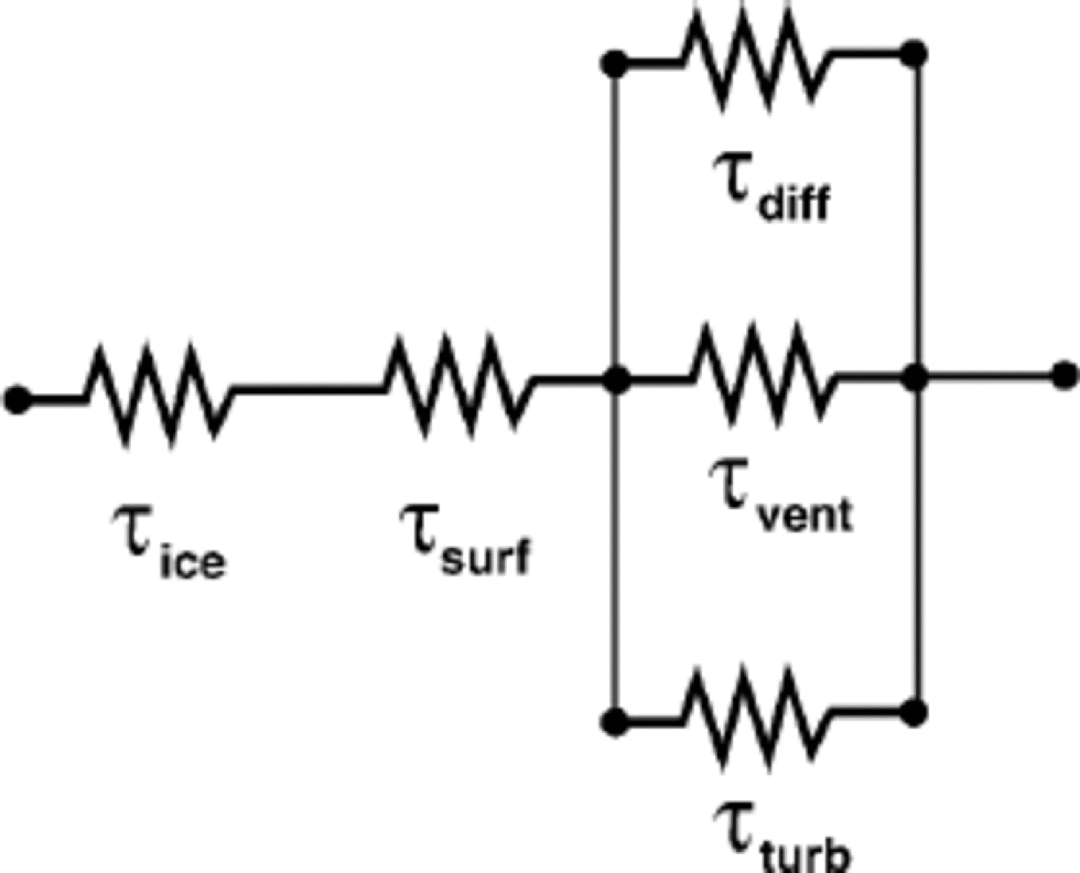
Fig. 1 Each process that delays isotopic equilibration with atmospheric vapor can be represented by a characteristic time τ that may depend on depth z . the total time required to equilibrate can be obtained by connecting the characteristic times for the contributing processes in a resistor network.
Here, we closely follow the method ofReference Waddington, Cunningham, Harder, Wolff and BalesWaddington and others (1996) to estimate the characteristic times for the relevant processes that can impede equilibration of stable isotopes. They showed that, as a series resistor, τsurf is typically too short to limit equilibration, and turbulent wind pumping τturb is too long in comparison to molecular diffusion and topographic ventilation times, with which it works in parallel, to affect equilibration rate. Therefore we restrict our analysis to the remaining three processes represented by τice , τdiff and τvent.
Diffusion within ice grains
Mixing of water molecules with different isotopic signatures within ice grains is controlled by the coefficient κice for self-diffusion which has a value of ≈ 5 × 10⁻⁸ m2 a–1 at –20˚C (Reference Whillans and GrootesWhillans and Grootes, 1985), and an Arrhenius temperature dependence with an activation energy for volume self-diffusion of 60.7 kJ mol–1 (Reference PatersonPaterson, 1994). Scaling arguments applied to the governing differential equation suggest that the characteristic time for diffusion in a grain with radius r is
G is a geometrical factor whose value is ≈ 0.057 (Reference Whillans and GrootesWhillans and Grootes, 1985). for a representative grain-size variation r(z) with depth z in polar snow, we use the solid curve in Figure 2, which is based on data from South Pole (Reference GowGow, 1969) and the East Antarctic plateau (Reference Stephenson and ŌuraStephenson, 1967). Grains are larger in warmer and less windy areas such as Greenland; Reference GowGow (1968) also reported larger grains in West Antarctica. to explore these conditions, we also use the dashed curve in Figure 2.
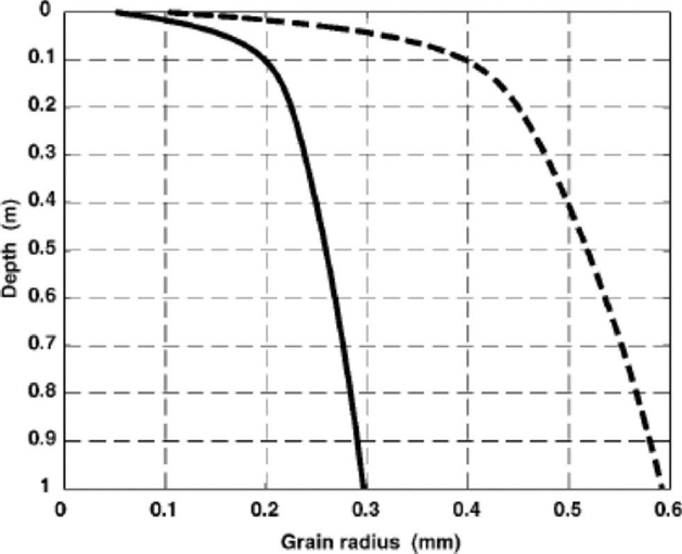
Fig. 2 Solid curve shows radius of snow grains in Antarctica, based on data by Reference Stephenson and ŌuraStephenson (1967) and Reference GowGow (1969). Larger grains (dashed curve) could be found at warmer or less windy sites, such as in parts of Greenland.
Molecular diffusion in pore spaces
Polar firn canbe described by its permeability K, porosity ϕ and temperature T. Water vapor in air has a diffusion coefficient κair that depends on T1.75 (e.g. Reference Whillans and GrootesWhillans and Grootes, 1985). In firn, where pathways are blocked by ice grains, the diffusivity diminishes with depth. Reference Schwander, Oeschger and LangwaySchwander (1989) found that the diffusivity κair diminished from ≈ 10–5 m2 s–1 near the surface, to vanishingly small values near the pore close-off depth. Theoretical treatments by Reference Whillans and GrootesWhillans and Grootes (1985) and Reference Cuffey and SteigCuffey and Steig(1998) derived similar values by accounting for blockage of vapor diffusion pathways by ice grains. In the current state-of-the-art treatment, Reference Johnsen, Clausen, Cuffey, Hoffmann, Schwander, Creyts and HondohJohnsen and others (2000) derived κair from first principles, with no adjustable parameters, by including measured tortuosity
factors for firn. the characteristic time for water vapor that is already in the pore spaces to equilibrate with the atmosphere (i.e. for a single air exchange) is then
However, many air exchanges are required, because of the large reservoir of water molecules within the ice grains in a unit mass of snow, relative to the number of molecules in the vapor phase.The required number n of air exchanges scales with the ratio of the amount of ice to the amount of pore vapor, i.e.
where ρice, ρair and ρvapor are densities of ice, air and water vapor, ϕ is porosity, Pair is air pressure at the site, and es(T ) is saturation vapor pressure over ice at temperature T, given by the Clausius–Clapeyron equation. the required number of air exchanges rises rapidly as temperature decreases, because colder air is less able to carry water vapor. the characteristic time for firn at depth z to equilibrate with the atmosphere by molecular diffusion through the pore spaces is then
which suggests that the effective diffusivity κfirn for isotopes in bulk firn should be approximately κair/n. Values of κfirn in the literature on smoothing of annual isotopic signals in firn (e.g. Reference JohnsenJohnsen, 1977; Reference Whillans and GrootesWhillans and Grootes, 1985; Reference Cuffey and SteigCuffey and Steig, 1998; Reference Johnsen, Clausen, Cuffey, Hoffmann, Schwander, Creyts and HondohJohnsen and others, 2000) are very similar to our κair/n.
Forced ventilation
Wind blowing over microtopography (Fig. 3) sets up steady high and low pressures on the snow surface (Reference ColbeckColbeck,1989), and air flows steadily within the snow from the high-pressure to the low-pressure areas. By transporting water vapor, this steady airflow helps isotopes in the snow to equilibrate with atmospheric vapor.
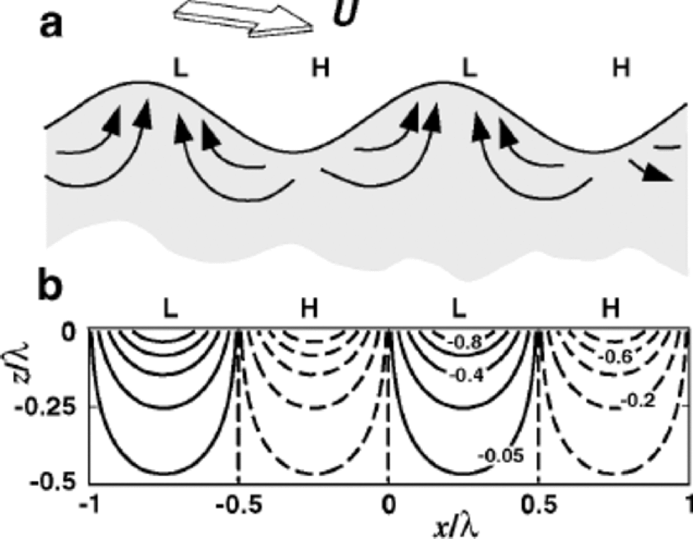
Fig. 3 (a) When steady wind flows at speed U over sastrugi, high pressures (H) are set up on the upwind slopes and in the hollows, and low pressures near the crests or leeward slopes. Air flows in the firn from H to L. (b) Isobars of the Reference ColbeckColbeck (1989) pressure perturbation solution in the firn normalized by p0 , half the pressure difference between H and L. Th . sinusoidal pressure perturbation is applied on a flat surface rather than on the actual topography. In the firn, air flows normal to the isobars.
To estimate the time required to flush the air out of the snow n times, we follow Reference ColbeckColbeck (1989), Reference Cunningham and WaddingtonCunningham and Waddington (1993) and Reference Waddington, Cunningham, Harder, Wolff and BalesWaddington and others (1996) by approximating the ice-sheet surface by a wavy interface with wavelength λ and amplitude h. With steady wind speed U at 10m above the snow surface, the pressure on the surface varies approximately sinusoidally, with an amplitude of
where C ≈3 (Reference ColbeckColbeck, 1989). to estimate the airflow through the snow, we apply a sinusoidal pressure variation with amplitude p0 on the surface of a permeable half-space. Figure 3b shows the non-dimensional analytical solution for pressure in the snow. the time for a single air exchange at depth z can be approximated by the time needed for air at that depth to move a distance λ, i.e. the span of a surface bump at the speed typical of depth z. the speed of airflow depends on air viscosity μ, snow permeability K and porosity ϕ. the characteristic time for a single air exchange at depth z (Reference Waddington, Cunningham, Harder, Wolff and BalesWaddington and others, 1996) is
Porosity of ϕ ≈ 0:6 is typical of near-surface snow. Reference Albert, Shultz and PerronAlbert and others (2000) found permeability of K ≈ 10–9 m2 for the upper few cm at Siple Dome, with higher values below a wind-packed surface crust. Now, we express the characteristic time τvent to equilibrate the isotopes in snow at depth z with the isotopic content of the atmospheric vapor by ventilation alone through
Forced ventilation has negligible impact on smoothing of seasonal isotopic variations in deep firn, due to the exponential increase of air-exchange time with depth in Equation (6). We take a conservative approach in adding this process; by applying the surface permeability to all depths, and using a relatively long airflow path along with the velocity at the deepest (and therefore slowest) point, we will tend to overestimate times required for equilibration, and to underestimate its importance.
Total equilibration time
To find the time τtotal that characterizes isotopic equilibration of snow at any depth z, we connect the process characteristic times as illustrated in Figure 1 to get
where we have used the approximations τsurf ≈0 and τturb ≈ ∞.
Results
In order to estimate isotope equilibration times on the polar ice sheets, we must first characterize the surface morphology and the climatology. Since τice and τdiff depend strongly on temperature, through the activation energy for volume self-diffusion, and through saturation vapor pressure, respectively, we anticipate that equilibration times will be much shorter in summer than in winter; therefore we focus on summer conditions while exploring the impact of temperature. We choose a standard snow surface and wind speed, and vary the temperature. We use a surface that has undulations with amplitude 2.5 cm and wavelength 25 cm. This roughness is compatible with a windy area; we use a wind speed of 10ms–1 at 10m height. This best represents sites on the slope of an ice sheet where katabatic drainage is strong. Ice-core sites on ridges or dome crests tend to have smoother surface and lighter winds. Later we examine the impacts of those differences.
Figure 4 shows the characteristic equilibration times in the upper 1m of snow for sites with this standard wind and microtopography, and with three different summer temperatures, –20˚, –30˚ and –40˚C. High-elevation sites in Greenland today could have an average summer temperature of –20˚C during the warmest month, while at Vostok the warmest month is close to –30˚C (World Meteorological Organization/Antarctic CRC data, courtesy of T. H. Jacka). A warmest month of –40˚C might better represent ice-age conditions. In each panel, the characteristic equilibration time τtotal at each depth is shown by the bold solid black curve, and the times for each of its contributing processes are shown by bold dashed grey curves. As expected, the time needed to equilibrate with the atmospheric vapor increases with depth for all processes: τice encounters increasing grain radius r(z) (Fig. 2), τdiff increases with z2 (Equation (4)), giving a straight line on a log–log plot, and τvent increases exponentially (Equation (7)), becoming negligible at depths on the order of λ, the wavelength of the microtopography. At all three temperatures, the equilibration time in the upper few mm tends to be limited by the time for isotopes to diffuse out of ice grains. Below about 1cm, the time to transport vapor through the pores becomes rate-limiting. In the depth range 1–30cm, forced ventilation dramatically shortens the equilibration time, compared to molecular vapor diffusion alone.
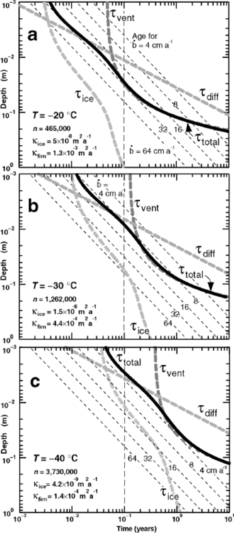
Fig. 4 Bold dashed grey curves show characteristic times as a function of depth in the snow for individual processes that contribute (see Fig. 1) to τtotal , characteristic time to reach equilibration (solid black curve). (a) T = –20˚C; (b) T = –30˚C; (c) T = –40˚C. the number n of air exchanges, the diffusivity κice in solid ice, and the effective firn diffusivity κfirn = κair/n vary with temperature. In all panels, wind speed is 10m s–1, grain-size is given by solid curve in Figure 2, and surface microtopography has 2.5 cm amplitude and 25 cm wavelength. Slanted thin dashed lines show the average depth–age relation for accumulation rates from 64 to 4 cm a–1 of snow.
The vertical dashed line in each panel shows a time of 0.1 year, or approximately 1month. In the absence of precipitation during the warmest month, snow that sits at depths where the characteristic equilibration time τtotal is <0.1year is likely to isotopically equilibrate with the overlying atmospheric vapor. Where T = –20˚C, this comprises the upper few cm, and ventilation significantly deepens the equilibrated layer. Where T = –40˚C, only the uppermost few mm could equilibrate in 1month. Vigorous ventilation cannot drive the snow to equilibrium, due to the large number n of air exchanges required at low temperatures. Dome-F Ice Core Research Group (1998) reported that more than 95% of the surface mass balance at Dome Fuji station was accounted for outside the summer season. This suggests that summer periods in which equilibration can proceed may be commonly longer than 1month.
Another way to interpret the equilibration times in Figure 4 is to look for depth intervals in which the equilibration time is shorter than the age of the snow. for those depth intervals, the snow probably has time to reach equilibration with atmospheric vapor. Conversely, when the time necessary for equilibration exceeds the age of the snow, it is unlikely to have equilibrated, nor is it likely to be able to equilibrate in the future as it gets buried yet deeper. the slanted thin dashed lines show the depth–age relation in the upper meter, for accumulation rates ![]() successively doubling from 4 cm through 64 cm of snow annually, if snow is deposited continually at a uniform rate. from this perspective, snow at T = –20˚C in the upper 4 cm could equilibrate in just over 1 month, which is less than its age for all accumulation rates less than 48 cm annually. Moreover, if the accumulation rate is 4 cm of snow annually, this equilibrated layer would represent the entire year’s snowfall. However, a relatively warm site is unlikely to have such a low snowfall rate, and only a fraction of the annual snow might equilibrate. the need to know the statistical distribution of seasonal snowfall would complicate interpretation, even with a full physical process-basedmodel. In central Greenland, with an accumulation rate of near 60 cm of snow annually, essentially all the snow gets buried too quickly to have an opportunity to equilibrate with summer atmospheric water vapor. When T = –40˚C, diffusion processes are slow, and equilibration again looks improbable, even in the uppermost few mm, if the accumulation rate exceeds 4 cm of snow annually.
successively doubling from 4 cm through 64 cm of snow annually, if snow is deposited continually at a uniform rate. from this perspective, snow at T = –20˚C in the upper 4 cm could equilibrate in just over 1 month, which is less than its age for all accumulation rates less than 48 cm annually. Moreover, if the accumulation rate is 4 cm of snow annually, this equilibrated layer would represent the entire year’s snowfall. However, a relatively warm site is unlikely to have such a low snowfall rate, and only a fraction of the annual snow might equilibrate. the need to know the statistical distribution of seasonal snowfall would complicate interpretation, even with a full physical process-basedmodel. In central Greenland, with an accumulation rate of near 60 cm of snow annually, essentially all the snow gets buried too quickly to have an opportunity to equilibrate with summer atmospheric water vapor. When T = –40˚C, diffusion processes are slow, and equilibration again looks improbable, even in the uppermost few mm, if the accumulation rate exceeds 4 cm of snow annually.
At some low-accumulation sites on the Antarctic plateau, interannual variabilitymay result in several seasons of low or zero net accumulation. In such cases, snow layers at the surface could remain exposed to summer conditions in several successive years, enhancing their likelihood of equilibrating with summer atmospheric vapor. Where average accumulation rate is low, the coefficient of variation of accumulation rate (standard deviation divided by the mean) can be relatively large, and some snow may be buried very quickly in infrequent storms without an opportunity to equilibrate, while other snow may stay exposed at the surface for long times. Ultimately, to quantify the average degree of isotopic equilibration will again require incorporation of the statistics of accumulation rate. Progress in determining these patterns for other purposes has been made by Reference McConnell, Bales and DavisMcConnell and others (1997) and Reference Van der Veen, Whillans and GowVan der Veen and others (1999).
In order to assess the impact of equilibrationon the stable-isotope record, we would also want to compare the mass in a given layer to the seasonal or annual mass budget. In East Antarctica, where annual accumulation is low, it is possible that a significant fraction of the annual accumulation may on occasion be exposed to at least partial equilibration with summer air.
Figure 5 explores the sensitivity of the equilibration times to conditions other than temperature. All three panels are variants of Figure 4b, using T = –30˚C. Figure 5 shows a site with much calmer winds, U = 2 ms–1. Due to the quadratic dependence of ventilation on wind speed (Equation (5)), ventilation plays virtually no role in the upper 10 cm, where molecular diffusion alone must handle the air exchanges. As a result, the depth to which equilibration might be expected is reduced by a factor of about 2. In Figure 5b, doubled grain-size impedes equilibration in the upper few mm where diffusion through ice is the controlling factor, but has negligible impact at greater depths. In Figure 5c, doubled roughness of the surface microtopography increases the depth of the equilibrated layer during a summer by 50%. Although the absolute depth is still in the 1–2 cm range, this difference points to the need for better observations and theory relating surface microtopography to local climate.
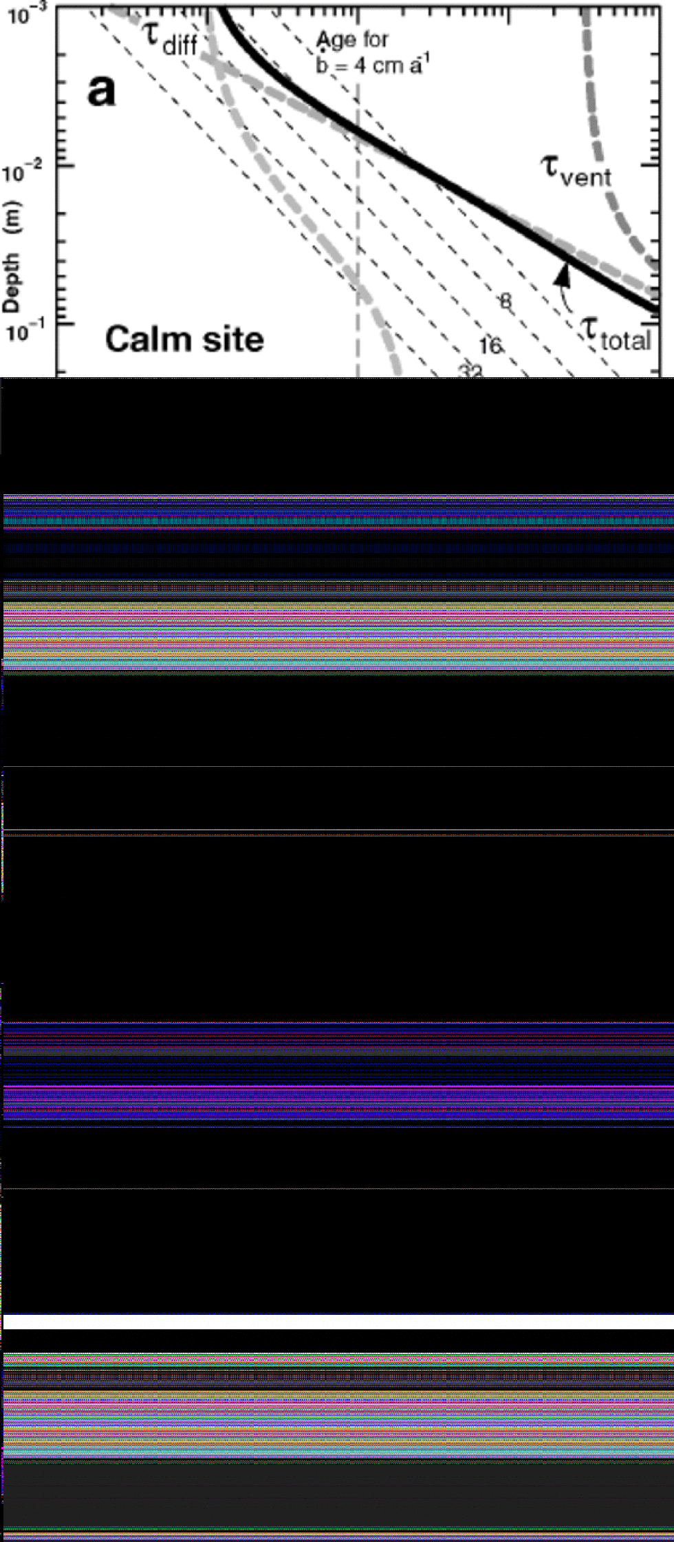
Fig. 5 Characteristic times τtotal to reach equilibrium as a function of depth, showing variants on Figure 4b. T = –30˚C in all panels. (a) Wind speed at 10 m height is reduced from 10 to 2ms–1; (b) the grain-size is doubled (dashed curve in Fig. 2); (c) the height of the microtopography is doubled.
This analysis can be applied to isotopic equilibrium in seasonal snowpacks, such as those studied by Reference Moser and StichlerMoser and Stichler (1975). Higher temperatures reduce the required number of air exchanges n, and decrease τice. Reference Moser and StichlerMoser and Stichler (1975) found that a significant fraction of a snow grain may sublimate and redeposit as hoar frost on diurnal time-scales. Consequently, it may be only the outer hoar layers on ice grains that reach isotopic equilibrium with the atmosphere. Our approach cannot easily represent this transient behavior; nevertheless, we note that total isotopic equilibrium of an entire snow grain with the atmosphere may still be limited by solid diffusion in the remaining core that does not cycle rapidly between the atmosphere and the snowpack. for T = –5˚C, U = 10ms–1, uniform radius of 1 mm at all depths z for the grain centers that do not sublimate or redeposit daily, and the same microtopography as used in Figure 4, our analysis predicts a characteristic time for equilibrium of ~2 months or less down to 7 cm in the absence of further snowfall. If the size of the inactive grain cores is 500 μm, the characteristic time is about 2 weeks. Although their isotopic composition will certainly change through time, as shown by Reference Moser and StichlerMoser and Stichler (1975), seasonal snowpacks will likely not be able to reach an equilibrium value, because the ``target’’ isotopic composition of the atmospheric vapor changes too rapidly for the snow-grain cores to respond, as weather systems bring new air masses past a site.
Discussion and Conclusions
There are several other important issues that our simple characteristic time approach has not allowed us to address. In particular, we assume that the environmental conditions are in steady state. Predicting changes in stable-isotope content in the presence of transients in temperature, grain-size or accumulation rate requires a process-based model of the isotopic system. Equilibration times may be shortened while grains are airborne or saltating in strong winds. Sublimation and redeposition within the snowpack as a result of grain metamorphism can enhance the release of isotopes from inside ice grains, and hasten their exposure to the summer atmosphere. This probably has a minimal effect on equilibration times, because τice is the rate-limiting factor only in the upper few mm. In polar snow, grain-size increases with depth (e.g. see Fig. 2), as larger grains grow by deposition of vapor sublimated off smaller grains. However, the growing grains may also incorporate new atmospheric vapor. Analysis by Reference NeumannNeumann (2001) suggests that the effect is likely to be small; however, quantifying this would require an isotope process model.
Can stable isotopes be reversibly deposited in polar snow? Our simple approach allows us to estimate the characteristic time associated with isotopic equilibration between snow and atmospheric vapor. We assume that equilibration processes can operate effectively only during a short summer period, and then compare characteristic times for isotopic equilibration to the amount of time that snow can be exposed to exchange processes, as a function of summer duration, summer air temperature, and accumulation rate and timing. We find that, in general, complete equilibration with summer vapor in the overlying atmosphere is unlikely, except under extremely windy, dry and relatively warm conditions, although some changes from the deposited values are possible. In dry, windy regions on the slopes of the East Antarctic ice sheet, near-surface snow may suffer significant modification. the impact is less at ice-core sites at summits such as Dome C, because the absence of katabatic winds results in a smooth surface and weak ventilation. Under the colder, drier conditions of an ice age, snow could remain longer near the surface, where it is exposed to ventilation; however, the decreased diffusivities and larger number of required air exchanges appear to offset this. In central Greenland, stable isotopes should faithfully retain their original composition, because high accumulation rate and rapid burial more than outweigh the enhancement of isotope exchange processes at warmer temperatures.
While our results can give a reasonable idea of where or when stable isotopes might be altered, each ice-core site has its own character, which cannot be fully represented in our temporal scaling analysis. the next question will be, how much can the isotopic ratios of bulk snow change? In order to determine the degree of equilibration at any particular site, a physically based model of isotope changes, driven by transient precipitation, wind, temperature and atmospheric vapor, should be used. Our analysis of characteristic time-scales primarily illustrates the rate at which we would expect to see changes occur in such a model.
As noted by Reference Cunningham and WaddingtonCunningham and Waddington (1993) and Reference Waddington, Cunningham, Harder, Wolff and BalesWaddington and others (1996), the microtopography of the snow surface is a key property that still lacks a systematic characterization applicable over large areas and a wide range of climates. Formation of microtopography also is imperfectly understood theoretically; this is an obstacle to predicting its character from climatology. Roughness elements with wavelengths of a few cm are the most efficient wind pumpers (Reference Cunningham and WaddingtonCunningham and Waddington,1993); however, large sastrugi are more easily noticed in remote-sensing imagery (and by snowmobile drivers!). Obtaining more measurements of the isotopic content and character of summer air masses over the polar ice sheets, and developing theoretical models of the physical air–snow interactions and the accompanying post-depositional isotopic changes(e.g. Reference NeumannNeumann, 2001) are two steps that must be addressed before the extent of post-depositional isotopic change at warm, windy or low-accumulation sites can be quantified.
Acknowledgements
Discussions with J. McConnell and R. Bale . stimulated our interest in reversibly deposited species in polar firn, and K. Cuffe . provided valuable insights into isotopic processes. We thank two anonymous reviewers and our scientific editor, S. Johnsen , for helpful comments. This work was supported by U.S. National Science Foundation grant OPP-0196085 and University of Washington Royalty Research Fund grant RRF-2503.


