1. Introduction

The sea-ice zone of the Southern Ocean plays an integral role in both local and global climate; however, it remains relatively data-sparse in terms of long-term climatological data. Only in the past two decades have comprehensive field programmes been undertaken to investigate Antarctic sea-ice properties and the interaction between the ocean, ice and atmosphere (e.g. Reference GordonGordon and others, 1993; Reference McPheeMcPhee and others, 1996; Reference Worby, Bindoff, Lytle, Allison and MassomWorby and others, 1996b) One of the most important, yet most difficult, parameters to measure is sea-ice thickness and its distribution. Reference Allison and MoritzAllison and Montz (1995) state that knowledge of the thickness distribution is of the highest priority for understanding the role of sea ice in the coupled atmosphere-ice-ocean system, and for detecting any variation in the ice due to climate change.

Numerous techniques have been used in recent years to determine Antarctic sea-ice thickness. These include drilled measurements (e.g. Reference AckleyAckley, 1979; Reference Wadhams, Lange and AckleyWadhams and others, 1987; Reference Lange and EickenLange and Eicken, 1991; Reference Worby and MassomWorby and Massom, 1995), electromagnetic induction sounding (Reference HaasHaas, 1998; Reference Worby, Griffen, Lytle and MassomWorby and others, 1999), upward-looking sonar (ULS) (Reference Strass, Fahrbach and JeffriesStrass and Fahrbach, 1998) and ship-based observations (e.g. Reference Worby, Massom, Allison, Lytle, Heil and JeffriesWorby and others, 1998). Additionally, submarine sonar profiling has been used in the Arctic (e.g. Reference Rothrock, Yu and MaykutRothrock and others, 1999). Each of these techniques is limited either spatially or temporally, and none come close to providing the extensive coverage of satellite sensors from which other parameters such as ice concentration can be determined. The use of satellite data for determining sea-ice thickness has been investigated by numerous authors, particularly with passive microwave data (e.g. Reference Eppler and CarseyEppler and others, 1992); however, no unambiguous relationship between irradiance fields and ice thickness is known, and ice thickness can only be inferred indirectly from surface properties. Reference Massom, Comiso, Worby, Lytle and StockMassom and others (1999) showed that an unsupervised ice-classification scheme using data from four Special Sensor Microwave/Imager (SSM/I) (passive microwave) channels provides valuable information on ice types; however, ambiguities are still observed. Using higher-resolution synthetic aperture radar (SAR) data, Reference Wadhams, Comiso and CarseyWadhams and Comiso (1992) showed that there is some correlation between backscatter values and ice draft, but the relationship is indirect and certainly not accurate enough to detect interannual changes. Ship-based observations such as those presented by Reference Worby, Massom, Allison, Lytle, Heil and JeffriesWorby and others (1998) provide useful spatially averaged data on the ice-thickness distribution, but these are not accurate enough for climate-change research and are temporally limited.

Moored ULSs are emerging as a practical means of measuring sea-ice draft, and subsequently ice thickness, despi a number of generic problems, particularly when deployed in the Antarctic. The large icebergs which drift through the Antarctic sea-ice zone present a significant hazard to ULS moorings (losses to date are approximately 50%), and require the ULS to operate from a depth approaching 200 m. The ULS instrument, located at the top of a mooring line, transmits an acoustic pulse toward the surface, and from its return travel time the distance between the instrument and the ice surface above can be determined. Sea-ice draft can then be calculated as the pressure-measured depth of the instrument minus the acoustic range to the ice surface. The difference between the simultaneous pressure measured depth of the instrument and the acoustic range to the ice/water interface is referred to as the residual distance. In the absence of surface gravity waves and errors this residual is the sea-ice draft. However, a large error, termed the residual offset, occurs in the residual calculation because of uncertainties in the density and sound speed of the water column above the ULS. The residual offset fluctuates with the temperature and salinity of the water, and can therefore be expected to vary seasonally, and at much shorter time-scales in response to vigorous surface forcing. It must be corrected by frequently identifying the occurrence of open water from echo properties, with each occurrence equivalent to a zero draft-calibration point.

ULS instruments have been deployed widely, and with success, in the Arctic (e.g. Reference Melling and RiedelMelling and Riedel, 1996; Reference Vinje, Nordlund and KvambekkVinje and others, 1998). In the Antarctic, Reference Strass, Fahrbach and JeffriesStrass and Fahrbach (1998) reported on six instruments that were moored across the Weddell Sea between the tip of the Antarctic Peninsula and Kapp Norvegia, and provided a seasonally varying time series of ice draft for the inflow and outflow of the Weddell gyre. The modal draft values from the ULS data were shown to be within the range reported by drilled measurements; however, the mean values were significantly higher, resulting from the more gradual tailing of the probability density distributions. Strass and Fahrbach dismiss spurious data or iceberg fragments as the cause of this, and propose that previously published drill data under-represent heavily deformed ice fields. This issue with drilled data has also been raised by other authors (e.g. Reference Worby, Jeffries, Weeks, Morris and JañaWorby and others, 1996a; Reference WadhamsWadhams, 1998) who claim that drill-hole data are not representative of the extremes of ice thickness and hence do not adequately represent the shape of the ice-thickness distribution, g(h). Even with unbiased drillhole sampling it is necessary to have a large sample to obtain an accurate estimate of the true mean ice thickness. As noted by Reference Rothrock and UntersteinerRothrock (1986) for the Beaufort Sea, a sample of more than 60 fully independent drillholes would be required to reduce the standard deviation of the mean ice thickness to 0.3 m.

2. Data Collection and Processing

The ULS instrument used in this study was a prototype designed and built at the Centre for Marine Science and Technology, Curtin University, Western Australia. It used a Reson SystemsTC2078 acoustic transducer with a centre frequency of 300 kHz and a beamwidth (−3 dB) of 2.5°. The acoustic range was measured to a resolution of 1.2 cm, and pressure depth to a resolution of 1.0 cm. To improve signal-to-noise ratio and enable the instrument to operate at up to 200 m depth (below most iceberg keels), the transmitted signal was modulated with a 31−bit pseudo-random binary sequence of phase shift and the received signal was correlated against a replica of the transmit signal. Pressure was measured with a Paroscientific Digiquartz 31X-101−1138−001−0 transducer. During the winter the instrument was programmed to transmit every 5 min in a two-stage process. Firstly a 1ms long tone burst (the narrow-band burst) was transmitted and received with a 1kHz one-sided bandwidth and sampled at 3 kHz. This signal was used to range to the target (24 cm resolution). Then the modulated signal (wide-band burst) was transmitted and received with a 20 kHz bandwidth and sampling frequency of 62.5 kHz (1.2 cm resolution). The data were stored on a 1 Mb EEPROM. To provide data to develop an open-water detection algorithm, the instrument was scheduled to record the integrated energy of the sonar echo every sixth draft measurement, the signal standard deviation every 6 h, and to make a multi-ping measurement (three rangings in quick succession) every 12 h. Further details of the instrument are given by Reference BushBush (1997).

This instrument (named SOFAR) was deployed in January 1994 at 63° 18’ S, 107°49’ E, off the continental shelf of Antarctica in 3260 m deep water. The instrument transducer was at 150 m depth. The instrument was recovered in January 1995. Some difficulties were experienced with the data recovery of this prototype instrument. In particular, the sea ice had a lower than expected acoustic scattering coefficient, and the sonar operated on the limit of its ranging capability. Reference Bush, Duncan, Penrose and AllisonBush and others (1996) later made in situ measurements and showed that the acoustic scattering coefficient of Antarctic sea ice was up to 10 dB less than published data from the Arctic had suggested. Consequently, data were lost at a rate that fluctuated over the year, but with a strong correlation to the satellite-derived daily open-water concentration as shown in Figure 1. The correlation exists because to first approximation the acoustic backscatter from open water was sufficient for the ULS receiver to operate, while that from the sea ice was not. During the period August-November the sonar-data return rate was consistently higher than the open-water concentration, confirming that a significant quantity of the received signals originated from sea ice. The seasonal variation in return rate from the ice is consistent with growing sea ice being a weak scattering surface because of the dendritic crystal structure at the ice/ water interface (Reference Jezek, Stanton, Gow and LangeJezek and others, 1990; Reference Bush, Duncan, Penrose and AllisonBush and others, 1996). This has the potential to bias the resulting histograms towards strongly scattering (i.e. melting) ice.

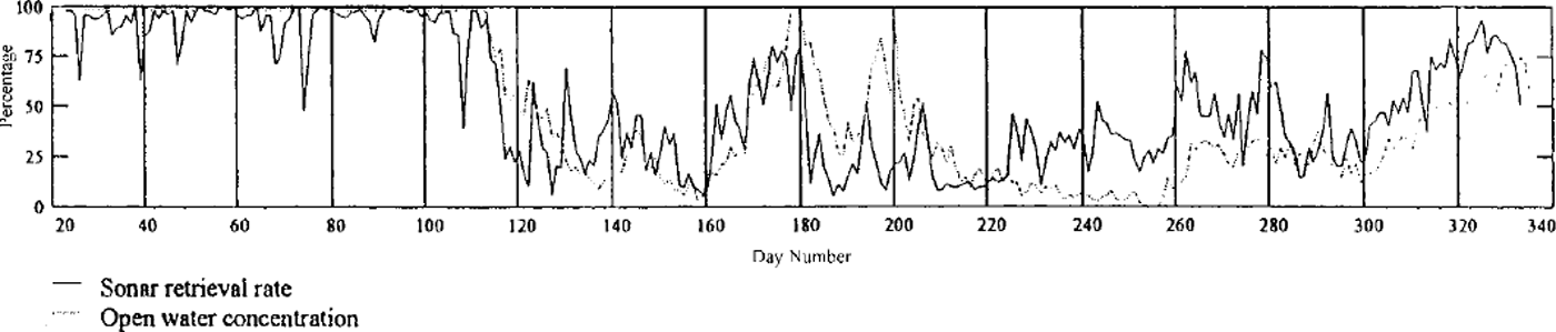
Fig. 1. Time series of uls retrieval rate and open-water fraction at the uls site, as determined from ssm/idata.

From the data recorded on this first deployment it was not possible to classify individual residuals from open water or sea ice. However, because of the low acoustic scattering coefficient of the ice, most of the recorded residuals were from open water. Hence we were able to estimate the residual offset and then separate the corrected residuals into open-water and sea-ice histograms by analyzing the data statistically. As a first estimate, the residual offset was calculated as the running mean of 20 small residuals (<1m), and the residuals were then corrected by this approximate offset. A second running mean was then calculated with a tighter condition (<∼0.4 m) on the size of the corrected residual. A third iteration was made before the estimated residual offset stabilized. The 20 small residuals typically corresponded to a time-scale of about 4 hours, so there will be some smoothing to the estimated residual offset time series. However, the residual offsets calculated from open-water summer months, when higher data return resulted in an averaging period of typically 2 h, indicate that the smoothing was not unreasonable.

The inclusion of some sea-ice residuals within these running means was unavoidable. To correct for this, the residual offset time series for each month was further reduced by up to 5 cm. This correction was chosen so that the peak of the corrected residual histogram (combined ice and open water) was at or just above zero. This assumes that the small sea-ice residuals included in the calculation of the residual offset were evenly distributed among the open-water residuals. The time series of corrected residuals was closely inspected for extended periods of "mistaken" open water that might be identified by an asymmetric appearance. No such events were identified.

Open-water and sea-ice histograms were then separated by assuming the open-water histogram was symmetric about the origin, being the result of surface gravity waves, and that sea-ice residuals had no occurrence less than zero. Natural fluctuations from the perfect symmetry assumed for the open-water residual directly affect the calculated sea-ice draft, and consequently ice-draft occurrences below about 0.3 m are considered inaccurate. The occurrence of residuals above 4 m was so infrequent that occasional false signals from the echo sounder would have affected the statistics, and these have been omitted from the histograms.

3. Results and Discussion

The ice-draft distributions derived from ULS data, and normalized between 0.3 and 4.0 m, are presented in Figure 2 and summarized in Table 1. These clearly show the seasonal development of pack-ice conditions from May through October. The ULS site during summer is completely ice-free, so it is not surprising that in May, early in the growth season, the distribution shows predominantly thin ice with only a very small fraction >1m thick. The mean draft is 0.59 m. The distribution injune is similar, although with a significantly higher fraction of ice in the 1−2 m thickness category as a result of deformation. The mean draft injune is 0.78 m. No data are available forJuly, due to low returns primarily caused by wave action (Reference BushBush, 1997); however, by August the distribution shows a substantial increase in the thicker categories, with 50% of the drafts > 1.0 m. This is consistent with the development of the pack ice due to deformation. Unlike the Arctic, where sea ice may grow thermodynamically to several metres, Antarctic pack ice usually deforms well before it reaches its thermodynamic maximum. Results from many core analyses in the East Antarctic region (Reference Worby and MassomWorby and Massom, 1995) clearly show that pack ice > 1 m thick is almost exclusively the product of deformation. The mean ice draft reaches a maximum of 1.21 m in August, which is consistent with the peak thickness observed from ship-based observations (Reference Worby, Massom, Allison, Lytle, Heil and JeffriesWorby and others, 1998).

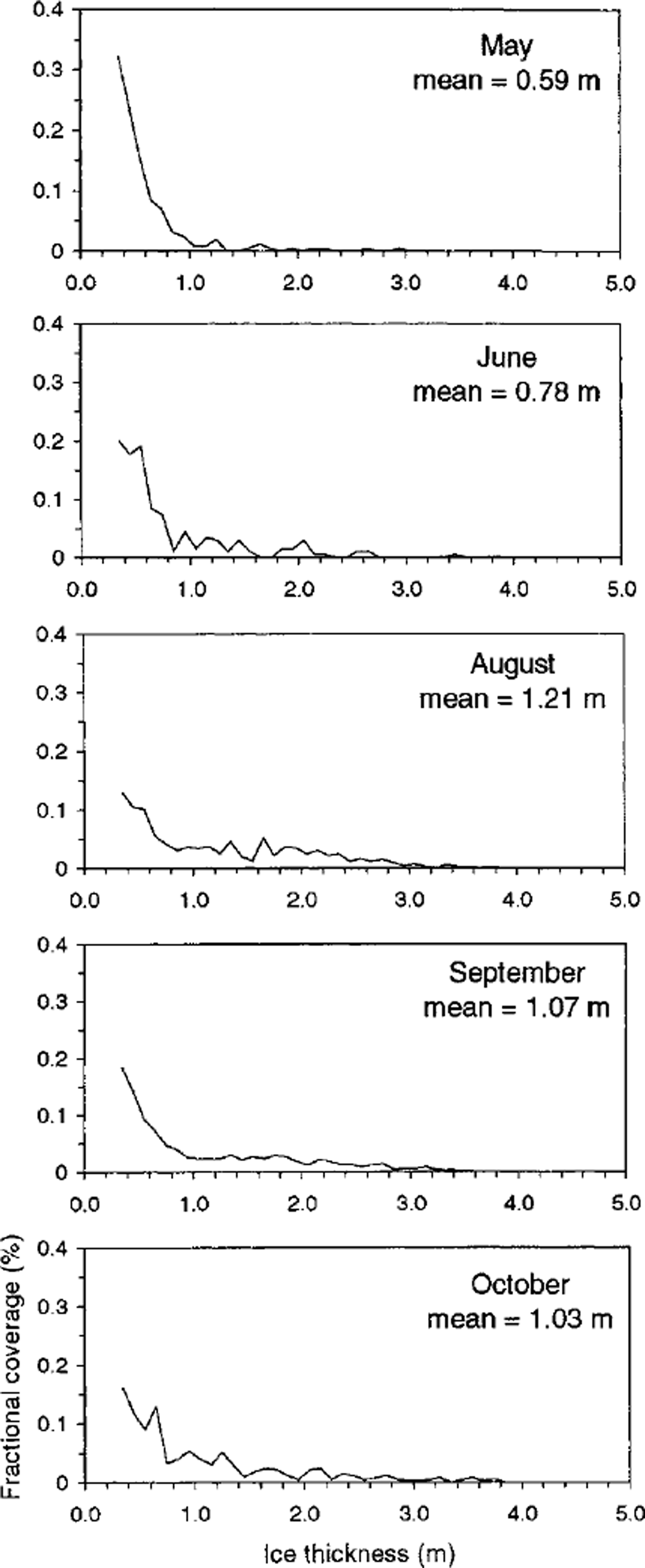
Fig. 2. Ice-draft distributions, normalized between 0.3 and 4.0 m from uls data.

Table 1. Percentage of ice drafts in each thickness category by month

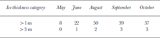
From August to October the mean ice draft decreases to 1.03 m and the percentage of drafts > 1.0 m decreases to 37%, a trend which is also consistent with the ship-based data. What is particularly interesting is the lack of development of substantially thicker ice during the spring. From August through October the percentage of drafts >3.0m remains constant at 2−3%, thus truncating the tail of the distribution curve. This is in contrast to observations in the Arctic where the distribution more closely approximates a negative exponential (Reference Wadhams and DavyWadhams and Davy, 1986). The formation of very thick ice requires sustained pressure in highly compact ice, and since the East Antarctic pack ice undergoes cyclical periods of divergence and convergence (Reference Worby, Bindoff, Lytle, Allison and MassomWorby and others, 1996b), conditions conducive to extreme deformation rarely occur. New ice is formed during periods of divergence and then compressed into moderately thick ridges during compression. Major divergence/convergence events in the East Antarctic pack occur with the passage of cyclonic systems with a period of 18−20 days (Reference Jones and SimmondsJones and Simmonds, 1993; Reference Heil and AllisonHeil and Allison, 1999), but there is also significant sea-ice deformation in sub-daily processes associated with inertial and/or tidal motion (Reference Heil and AllisonHeil and Allison, 1999). Hence, the sustained pressure required to produce much thicker ice rarely occurs, and the distribution curve maintains some uniformity during the spring period. This was also shown in the thickness-distribution curves derived from ship-based observations (Reference Worby, Massom, Allison, Lytle, Heil and JeffriesWorby and others, 1998). Reference ThorndikeThorndike (2000) noted that the tail of the thickness distribution arises by piling ice upon itself in a sequence of events each of which has a low probability; hence, to obtain very thick ice requires a sequence of improbable events to occur. Since the ice in this region of the Antarctic pack is wholly first-year ice, and thus has a particularly short lifetime, such sequences of "unlikely events" rarely occur and the tail of the distribution curve is truncated as a result. In the ULS record, peaks > 4 m were so few that they could not be distinguished from occasional bad echoes and were consequently removed.

4. Conclusions

ULSs are the most useful tool currently available for measuring the seasonal evolution of the sea-ice thickness distribution in Antarctica. The data presented here are from a prototype instrument deployed in 1994 and, despite some problems with the echo retrievals, provide useful information on the development of the ice-thickness distribution for the period May-October, with a data gap in July. Data loss caused by the low acoustic reflectivity of vigorously forming ice resulted in distribution curves that represent only ice drafts >0.3m. This problem has been addressed by the improved performance of subsequent instruments. The monthly draft distributions clearly show the seasonal development of the pack ice, from predominantly new thin ice in May to a broader range of thickness categories, including deformed ice up to 4 m thick, in spring. The peak in ice thickness is observed in August, consistent with the results of ship-based observations from the same region; however, the typically long tail of the distribution curve often observed in the Arctic never develops. This lack of extreme ridging is a common feature of the East Antarctic pack ice caused by the cyclical nature of deformation events, and lack of sustained pressure needed to create substantially thicker ridges.