


1. Introduction
The greenland sea (gs) and barents sea (bs) wintertime sea-ice cover is very variable and can change by about 300 000 and 200 000 km2 respectively within 2–3 years (Reference WadhamsWadhams, 1981; Reference ToudalToudal, 1999). it is determined by the surface airflow, the ice conditions upstream, i.e. north of the fram strait, and the oceanic heat transport. the geographical position of the ice edge, the ice-concentration distribution within the ice-covered area and the amount of ice formed/melted influence the local hydrography, and are important for water mass transformation in the gs (Reference Karstensen, Schlosser, Wallace, Bullister and BlindheimKarstensen and others, 2005), in the bs (Reference Schauer, Loeng, Rudels, Ozhigin and DieckSchauer and others, 2002) and further downstream (Reference Zhang, M., Rothrock and LindsayZhang and others, 2004). the ice cover influences the tracks and intensities of cyclones in this region and on the eurasian and siberian shelves, which affects, for example, the surface salinity (Reference Steele and ErmoldSteele and ermold, 2004). analyses of the regional and temporal change of the gs and bs ice covers have been made (Reference ToudalToudal, 1999; Reference Parkinson and CavalieriParkinson and cavalieri, 2002). however, these studies lack details about changes in the sea-ice compactness within the ice-covered area (e.g. whether an observed decrease in the ice area is simply caused by a loss of very compact sea ice (>95%)). this paper utilizes daily sea-ice concentrations of the period 1979–2003 obtained from space-borne microwave radiometry in the gs and bs to calculate the total sea-ice area and extent, and the percentage sea-ice area and extent fractions of certain ice-concentration ranges relative to the total sea-ice area and extent. trend analyses are carried out for these quantities over the given period. the results are qualitatively compared to the surface wind vector fields obtained from 40 year european centre for medium-range weather forecasts (ecmwf) re-analysis data (era-40) in order to investigate the link between the observed changes in the ice cover and in the surface airflow.
2. Data
The sea-ice concentrations are taken from d.j. cavalieri and others (http://nsidc.org/data/nsidc-0002.html) for the period 1978–2003. this dataset comprises daily sea-ice concentrations calculated with the nasa-team algorithm (nt) and projected into a polar stereographic grid with 25km×25km gridcell size using brightness temperature measurements by the space-borne microwave sensors scanning multichannel microwave radiometer (smmr) and special sensor microwave/imager (SSM/I). this dataset includes inter-sensor calibrations, the removal of land spillover effects, and a weather filter to remove false ice over the open ocean (d.j. cavalieri and others, http://nsidc.org/data/nsidc-0002.html).
The accuracy of nt ice concentrations is 2–5% for consolidated ice for the arctic during winter (Reference CavalieriCavalieri and others, 1991; d.j. cavalieri and others, http://nsidc.org/data/nsidc-0002.html). this accuracy declines to 10–25% during summer melt and towards smaller ice concentrations which are typical in the marginal ice zone (miz). comparisons with other ice-concentration retrieval algorithms (e.g. the comiso bootstrap algorithm (cb)) show generally good agreement in the arctic during winter over pack ice. mean differences and standard deviations are similar when comparing nt and cb ice concentrations to those derived from independent satellite observations such as the us national oceanic and atmospheric administration (noaa) advanced very high resolution radiometer (avhrr). larger discrepancies, however, arise in the miz (and in the antarctic) (Reference Comiso, Cavalieri, Parkinson and GloersenComiso and others, 1997; Reference MeierMeier, 2005). Reference MeierMeier (2005) showed that relative to ice concentrations derived from avhrr imagery, nt ice concentrations are 6% lower than cb ice concentrations in the gs, and that they are similar to cb ice concentrations in the bs for winter 2001/02. Reference Comiso, Cavalieri, Parkinson and GloersenComiso and others (1997) reported that nt ice concentrations were 5–10% lower than cb ice concentrations in the bs and gs for winter 1991/92. maximum differences tend to appear close to or in the miz. however, according to Reference Comiso, Cavalieri, Parkinson and GloersenComiso and others (1997), nt ice concentrations are less sensitive to temperature fluctuations. this is an advantage when investigating the ice cover of the gs and bs, where cyclonic activity can cause rapidly fluctuating air and surface temperatures. therefore, despite the fact that the examples given above indicate an underestimation of nt ice concentrations relative to cb ice concentrations, we took the nt for our analysis. we focus on ice concentrations >65%, i.e. not on the miz where errors tend to be largest.
We calculated the daily ice extent (sum of the area of all ice-covered gridcells with >0% ice concentration; one gridcell ≈ 625 km2) and area (sum of the area of all ice-covered gridcells with >0% ice concentration weighed by the actual ice concentration). we note here that using 0% as the lower threshold might introduce an overestimation of area and extent compared to previous studies (e.g. Reference Parkinson and CavalieriParkinson and cavalieri, 2002). however, we focus on a long-term study of the pack ice and its compactness and not on the miz or ice edge. data gaps are filled via linear interpolation (smmr data are available every other day). this calculation is done for each day for the gs and bs as defined by the section masks given in d.j. cavalieri and others (http://nsidc.org/data/nsidc-0002.html) except that the kara and barents seas are considered separately and that the irminger sea is excluded (see fig. 1). for each of the two regions, not only the total area and extent are computed but also the fractions of the total area and extent that are covered by ice in the following ice-concentration ranges: <35%, 35–65%, 65–85%, 85–95% and >95%. this permits us to deduce how much of the area or extent of the gs or bs is covered by, for example, very compact sea ice (>95% ice concentration). as the fractions refer to the total area or extent of the gs or bs throughout the paper, henceforth we refer to area or extent fractions.
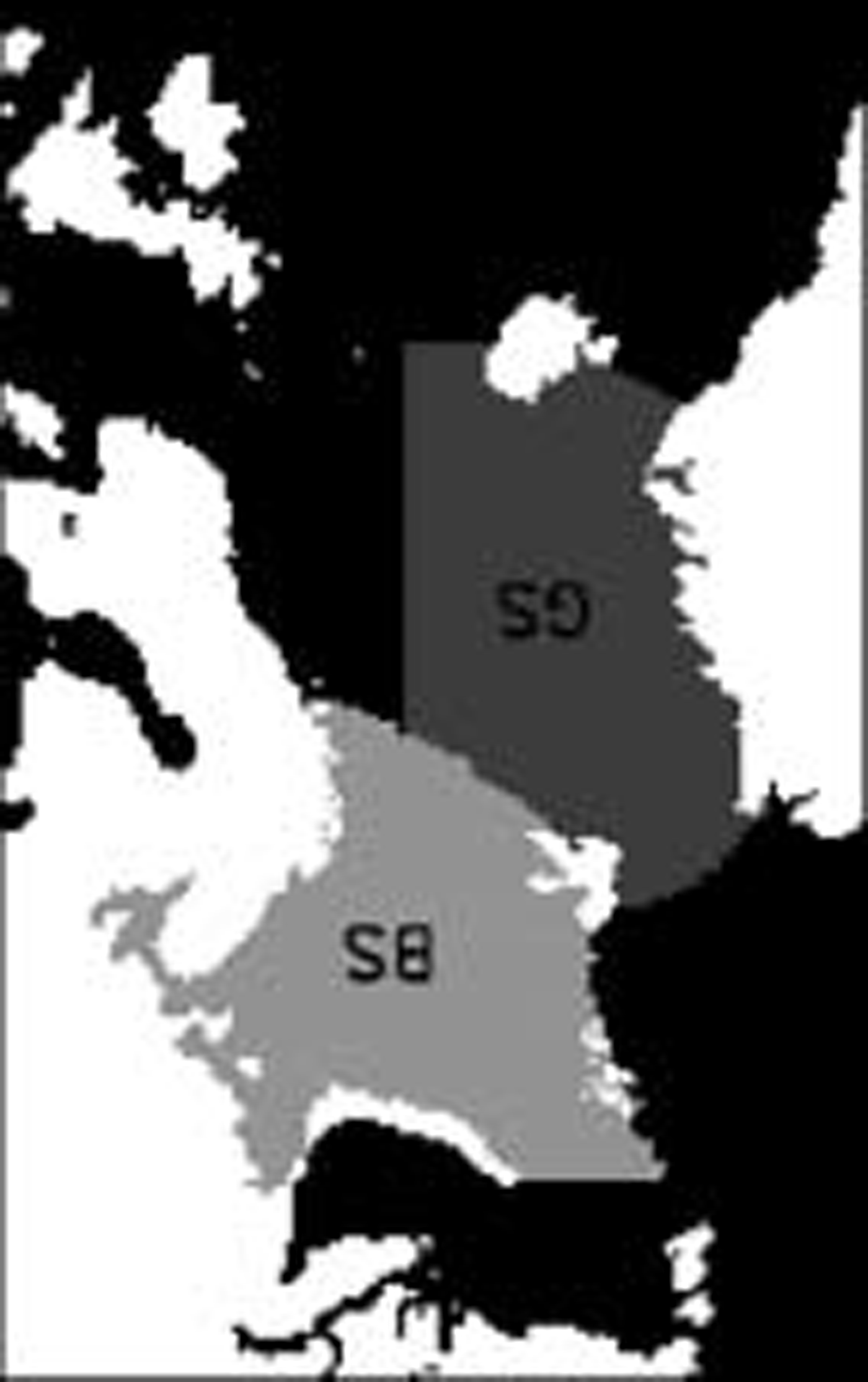
Fig. 1. Location of the study regions Greenland Sea (GS) and Barents Sea (BS).
What is the error of these fractions associated with the accuracy of the ice concentration? typical values for the total gs ice extent and the fraction of ice with >95% ice concentration are 700 000km2 and 20%, i.e. 140000km2. the accuracy of the ice concentration is about 2% in this range. let us assume that about one-half of the ice concentrations are <97%. this portion has a considerable probability to fall into the range 85–95%, which we estimate after some weighing to be approximately 20%, i.e. 28 000 km2. however, ice concentrations in the range 85–95% also have a considerable probability to fall into the range >95%. with realistic values for the ice-concentration accuracy, 2–5% (85–95%), 5–10% (65–85%) and 15% (35–65%), and typical numbers for the average relative fraction of the respective ice-concentration range (20%, 30%, 20%, 15%, 15% for the gs for ranges >95%, . . ., <35%), we estimate that the relative accuracy of each ice-extent fraction is similar to the average relative fraction itself. for the fraction of ice with >95% ice concentration, this value is 140 000 km2±20%, i.e. 140 000±28 000 km2.
The surface wind speed and direction are taken from era-40 data (u- and v-component). era-40 uses a state-of-the-art analysis/forecast system to perform data assimilation (http://www.ecmwf.int). the t319 truncation of the era-40 model is applied here, so that the spatial resolution is 0.5˚ latitude/longitude; the time resolution is 6 hourly data. no further processing is performed, except that mean monthly wind vectors are calculated.
3. SEA-ICE Area and Extent
Annual and winter (december–april) mean sea-ice area and extent are calculated for 1979–2003. a trend analysis is made based on these mean values, assuming that the main contribution to a trend over this 25 year period is linear. figure 2a and b show the weekly (daily values would be too variable to be shown in this graph), mean winter and mean annual ice extent for the gs and bs respectively, including trend lines calculated for the mean extents. both datasets show a periodicity of 5–10 years in the mean values and in the maximum winter extent. we consider the time series is still too short to allow use of a non-linear model to calculate the trends. moreover, it has been suggested by w. maslowski (personal communication, 2005) that models and periods used to calculate trends should be chosen according to the physical processes involved (e.g. different atmospheric circulation regimes as given by the north atlantic oscillation index). following this suggestion, one would calculate trends for the periods before 1991/92; 1991/92–1997/98; and after 1997/98. however, the time series given in figure 2 seem not to justify such a separation.
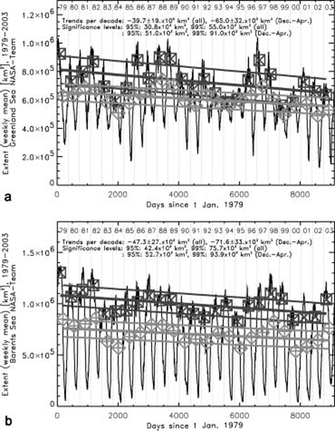
Fig. 2. Weekly average sea-ice extent of the GS (a) and BS (b), 1979–2003 (thin black lines). Light grey diamonds (dark grey squares) denote annual (winter: December–April) averages; thick grey lines give the trends of these averages calculated via linear regression for this period; and parallel thin grey lines denote one standard deviation of the linear model. Years and details of trends (in 103 km2) and significance levels are given at the top. Note the different scale of the vertical axis between (a) and (b).
table 1 gives an overview of the total annual and winter sea-ice area and extent of the gs and bs averaged over 1979–2003 together with the trends of the total annual and winter ice area and extent as given by the diamonds and squares in figure 2. the total annual ice extent decreases in agreement with observations by Reference Parkinson and CavalieriParkinson and cavalieri (2002), as does the total winter ice extent (fig. 2; table 1). the decreasing trend of the total annual and winter ice extent in the gs and bs is significant at the 95% level. the total amount of the decrease corresponds to 16.5% and 16.7% of the annual gs and bs ice extent averaged over 1979–2003, respectively; corresponding values for the winter ice extent are 22.2% and 17.5%. corresponding trends in the ice area are also decreasing and are of the same order of magnitude at 95% significance level.
Table 1. Total mean (1979–2003) annual and winter area and extent for the GS and BS, and trends (per decade) of the total sea-ice area and extent calculated from annual and winter means, 1979–2003. All the trends are significant at 95%
4. SEA-ICE Area and Extent Fraction
figure 3 shows selected panels of the ice-extent fraction occupied by ice-concentration ranges >95%, 85–95% and 65–85% for the gs (left) and bs (right). this fraction is given as mean weekly (black lines), winter (december–april; dark grey squares) and annual (light grey diamonds) values. the trends of the winter and annual values calculated for 1979–2003 using a linear model are also plotted in each panel together with one standard deviation. table 2 shows the winter trends for all ice-concentration ranges mentioned in section 2. figure 3 and table 2 reveal changes in the winter ice-extent fraction in both regions, which are mostly significant at the 95% level. in the gs the area of very compact sea ice (>95%) has increased by 58% relative to the mean winter value for 1979–2003. at the same time, the area covered by ice concentrations in the ranges 35–65% and 85–95% has decreased by >50% relative to the mean winter values for 1979–2003. therefore, the gs exhibits a smaller area (by about 78000km2) covered with open to compact sea ice (35–95%), but a considerably larger area (by about 72 000 km2) covered with very compact ice, during winter now than 25 years ago. in contrast, the bs has less area covered with compact sea ice (>85%) by about 67% relative to the corresponding mean winter value for 1979–2003. this seems to be compensated by a larger area covered with ice of all other ice-concentration ranges (<85%). therefore, the bs exhibits a smaller area (by about 165 000 km2) covered with compact (>85%) sea ice but a larger area (by about 102 000 km2) covered with open to compact (35–85%) sea ice during winter today than 25 years ago. in summary, the winter ice cover in the gs has become more compact, that of the bs more open.
Table 2. Overview of the winter ice-extent fractions and their trends for the GS (left part) and BS (right part), 1979–2003. For every ice-concentration range the table shows: average total extent covered by ice of the respective fraction for 1979–2003, the trend of this fraction (including its standard deviation) per decade, the change due this trend relative to the 25 year average total extent, and the significance level (blank cells have significance level <95%)
5. Discussion
Errors in the retrieved ice concentration, caused, for example, by severe weather conditions (particularly high cloud liquid-water content), or ice surface properties that are different from those represented by the algorithm’s tie points (layering in the snow; surface crusts), take values of 2–5% over consolidated ice and up to 10–25% in the miz (section 2) during winter in the arctic. errors caused by weather are positive, i.e. ice concentrations are overestimated, and are not corrected by the weather filters used since these are applied over the open ocean only. errors caused by surface properties tend to be negative, i.e. the ice concentration is underestimated. the two errors may cancel each other. one can expect weather effects to dominate in the miz while surface effects dominate over consolidated ice. since we focus on ice concentrations >65% and winter conditions, the errors in the ice concentration are <10%, and the relative accuracies for the extent fractions discussed in section 2 seem reasonable. errors caused by deviation of the used gridcell size from the value of 625 km2 are small compared to the other error contributions.
Ice areas and extents (and fractions) are recalculated using cb ice concentrations (j.c. comiso, http://nsidc.org/data/nsidc-0002.html). the results agree with those derived using the nt, i.e. annual and winter area and extent decrease, although with less significance. ice-extent fractions, however, differ. the fraction of ice with >95% ice concentration is around 20% for the nt but 35–40% for the cb. fractions of the other ranges differ by 5% (85–95%; nt > cb) and 10% (65–85%; nt > cb). trends derived for winter ice-extent fractions using the cb tend to be reversed compared to using the nt but are less significant in the gs. in the bs, only the trend for the ice-concentration range 85–95% tends to be reversed relative to using the nt. however, when taking the standard deviations of the trends and the relative accuracy of the extent fractions (section 2) into account, the general conclusion of our study is that the gs ice cover has become more compact, and that of the bs less compact during the last 25 years. the results must be considered carefully, because of a potential ice-concentration underestimation by the nt, especially in the gs (section 2), which deserves further investigation in the future.
The gs and bs have different ice regimes. the gs is dominated by perennial ice, which is continuously imported through the fram strait. new ice forms in leads and in or along the miz (e.g. in the is odden (see below)). the bs is dominated by seasonal ice, except in the north where perennial ice may occur. consequently, the ice is thicker and mechanically more stable in the gs compared to the bs and may therefore withstand swell longer than in the bs. as a result, the ice cover can be destroyed and redistributed by wind and swell more easily in the bs than in the gs. the minimum summer ice extent, which determines the amount of perennial ice the following winter, has decreased over the past two decades (e.g. Reference ComisoComiso, 2002). the maximum southward ice extent has high interannual and regional variability: years with a large amount of ice in the northern bs or north of it at the end of summer (1987–89) interchange with years with no ice in this region at this time (1979) (Reference ComisoComiso, 2002). a qualitative comparison of the minimum summer ice extent and figure 2 reveals no correlation with the winter ice extent or ice-extent fractions (for ice concentrations >65%) in the gs or bs.
A particularly interesting feature of the gs is the is odden, a tongue of predominantly young sea ice extending east- to northeastward north of jan mayen and covering an area of up to 380000km2 (Reference Comiso, Wadhams, Pedersen and GerstenComiso and others, 2001). average (monthly or longer period) ice concentrations remain below about 80% in the odden. therefore, pronounced is odden events (1978/79, 1981/82, 1985/86–1988/89, and 1996/97 (Reference Comiso, Wadhams, Pedersen and GerstenComiso and others, 2001)) are expected to increase the winter ice-extent fraction for the ranges 35–65% and 65–85%. however, there is no evidence in the time series of these fractions for such an increase (see fig. 3e), because in six out of seven winters during 1978/79–1997/98 a large is odden ice extent (>300 000 km2) coincided with an above-average gs ice extent. therefore, although the ice-covered area in the ranges 35–65% and 65–85% might have increased during these winters, the relative contribution to the total gs ice extent remained unchanged.

Fig. 3. Percentage ice-extent fraction for ice-concentration ranges >95% (a, b), 85–95% (c,d) and 65–85% (e, f) for the GS (left) and BS (right). See Figure 2 for further details.
The most important and direct driver for the observed compactness changes is the surface airflow, considered in section 5.1. other important drivers, such as changing oceanic conditions (currents, heat transport, stratification), have been discussed elsewhere (e.g. Reference Zhang, M., Rothrock and LindsayZhang and others, 2004). also not investigated in this study is the change in ice compactness due to the random movement of ice floes and/or systems of floes. a less compact ice cover allows more random movement, and therefore a larger probability for ice floes to be redistributed and piled up by local currents, than a highly compact ice cover. the area fractions of compact and open ice would increase at the expense of the area fraction of open to compact ice as ice floes glue together or pile up. consequently, an increase of the fraction of very compact ice (as observed in the gs) could be caused by less compact ice upstream (e.g. in the fram strait); this might become the topic of a model study in the future.
5.1. Changes in the surface airflow
An increase in ice compactness can be caused by an increased convergent airflow towards the ice edge. a decrease in compactness can be caused by the reversal of this situation. in order to investigate whether the general pattern of the airflow has changed during the considered 25 year period, we chose two 5 year intervals at the beginning and end of this period to derive a 5 year mean winter surface wind-speed pattern. these 5 year intervals each cover a sample set of different ice extents and extent fractions (figs 2 and 3). figure 4 shows three panels each for the gs and bs with the 5 year mean winter surface wind speed of 1979/80–1983/84 (fig. 4a and d) and of 1997/98–2001/02 (fig. 4b and e), and the difference of the mean vectors of these two periods (fig. 4c and f). the most pronounced change in the generally southward airflow in the gs (fig. 4a and b) is a wind-speed increase by up to 3 ms–1 in the central/southeastern gs (as marked in fig. 4c). considering that the effective surface drag is at least 20–30˚ off the wind direction to the right in the northern hemisphere, this airflow change favours enhanced on-ice flow and therefore an ice compaction in the gs. in the bs, a northwestward shift of the belt of low wind speeds (which coincides with a belt of low surface pressure) northwest of novaya zemlya can be observed (ellipses in fig. 4d and e). as a consequence, surface wind speed has increased by about 2 ms–1 in the western/northwestern bs (black rectangle in fig. 4f) and in the eastern bs (grey rectangle in fig. 4f). most importantly, however, the surface wind direction has changed from northeast to east or even southeast in the eastern/northeastern bs. so the surface airflow over most of the bs has become divergent, favouring divergent ice motion and a less compact ice cover. in conclusion, the change in the general surface airflow pattern provides evidence for the observed long-term changes in ice compactness in the gs and bs.

Fig. 4. Mean 5 year winter surface wind-speed vector and its change in the GS (top) and BS (bottom) calculated from monthly averages of the u- and v-component taken from ERA-40 data. (a, d) are for winters 1979/80–1983/84; (b,e) are for winters 1997/98–2001/02; and (c,f) show the difference (b) – (a) and (e) – (d), respectively. The arrow in the lower right corner of each panel scales the wind vector. Plus symbols mark the mean 5 year 15% ice-concentration isoline. See text for rectangles and ellipses.
How does the sea ice react on the mean airflow during a single winter? we derived the mean winter surface wind-speed vector for 12 single winters (six for the gs and six for the bs) with exceptionally low or high compactness as indicated by figure 3. examples of the resulting pattern, being typical for either low or high compactness, are shown together with the average winter 15% and 85% ice-concentration isolines in figure 5 for the gs (fig. 5a and b) and bs (fig. 5c and d) for the winters indicated in each panel. in the gs, moderate northerly to northwesterly winds (about 0–10˚w; fig. 5a) are observed for winters with low ice compactness. strong northerly to northeasterly winds (about 0–10˚w; fig. 5b) are observed for winters with high compactness. so, in fact, a compact ice cover in the gs during winter seems to be associated with strong (7–11ms–1 maximum mean wind speed) northerly to northeasterly surface winds favouring enhanced on-ice airflow. the amount of perennial ice in the gs or in the fram strait at the beginning of the winter seems to have no influence, as was checked with the ice-extent maps by Reference ComisoComiso (2002). for the bs, northerly airflow spreading over almost the entire bs (fig. 5c) is observed for winters with large ice extent, and high compactness. in contrast, during airflow dominated by a cyclonic circulation in the bs (fig. 5d), the ice compactness tends to be low. this can be explained by an increasingly divergent ice drift and the fact that cyclones moving through the bs cause continuous change between ice advance/retreat and convergent/divergent ice drift and higher surface air temperatures. in contrast to the gs, the amount of perennial ice in or close to the bs seems to have an influence, especially during winters of predominantly northerly flow. in winters without perennial ice, the compactness is low, whereas in winters with such ice a high compactness is observed. one possible explanation could be that perennial ice stabilizes the ice cover and hampers its destruction (e.g. due to ocean swell) and that it causes colder surface air temperatures, which favour ice growth.
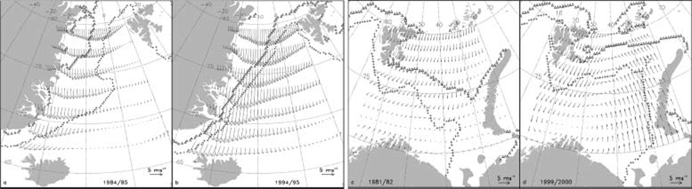
Fig. 5. Typical examples of the mean winter surface wind vector derived from ERA-40 data for two winters in the GS (a, b) and BS (c,d). The arrow in the lower right corner of each panel scales the wind vector. Plus symbols (triangles) mark the mean 15% (85%) ice-concentration isoline.
6. Conclusions
Daily sea-ice concentrations obtained from space-borne microwave radiometry for 1979–2003 are used to calculate the total annual and winter (december–april) ice extent for the gs and bs. ice-extent fractions (of these total extents) occupied by ice of five different ice-concentration ranges are calculated in order to examine changes in the ice-concentration distribution within the pack ice. the annual (winter) ice extent decreases significantly by 40000km2 (decade)–1 (65 000 km2 (decade)–1) and 47 000 km2 (decade)–1 (72 000 km2 (decade)–1) in the gs and bs, respectively. the largest significant trends in the ice-extent fraction also occur during winter. in the gs, the fraction of close to very compact ice (65–95%) decreases by 17 000 km2 (decade)–1, and the fraction of very compact ice (>95%) increases by 29000km2 (decade)–1. in the bs, the fraction of close to compact ice (65–85%) increases by 26000km2 (decade)–1, and the fraction of compact to very compact ice (>85%) decreases by 66000km2 (decade)–1. for the gs, this corresponds to a relative loss of 19% (gain of 58%) of the area covered by ice of 65–95% (>95%) ice concentration, relative to the 25 year mean. accordingly, the fraction changes in the bs amount to a relative gain of 30% (loss of 67%) for the area of 65–85% (>85%) ice concentration.
The winter ice compactness is a function of the surface wind pattern as is shown using era-40 data of 1979–2002 for a number of winters with low and high ice compactness. in the gs, low ice compactness coincides with moderate northerly to northwesterly winds, and high compactness is observed during strong northerly to northeasterly winds. the explanation is enhanced on-ice airflow during the latter. two major patterns are identified for the bs: northerly winds during which low and high ice compactness is observed, obviously depending on the amount of perennial ice; and a well-established cyclonic circulation during which low compactness is observed due to an on average divergent ice drift and less ice formation caused by higher air temperatures. the long-term increase (decrease) of the winter ice compactness in the gs (bs) during 1979–2003 might also be attributed to a change in the general surface wind pattern. this is indicated by changes in the 5 year mean of the wintertime surface wind-speed vector (also from era-40 data) at the beginning (1979–1983) and end (1997–2001) of the period 1979–2003, which favour similar changes in the ice compactness as is observed for single winters. because of the apparent influence of the amount of perennial ice on the bs ice compactness, we cannot exclude that the observed compactness change is caused by the decreasing minimum summer ice extent in the arctic rather than a changing surface wind-speed pattern.
We note that the general result of our study, i.e. ice compactness increase in the gs and decrease in the bs, has been obtained using ice concentrations of both the nt and cb algorithms. future work will aim at a quantitative comparison between ice compactness and atmospheric and oceanic surface heat fluxes. particular goals are to investigate melt rates of the sea ice during spring/summer, and to investigate the spatial pattern of the compactness change in relation to atmospheric and oceanic parameters.
Acknowledgements
This work was supported by the german science foundation (dfg): sfb 512-e1. the helpful comments of three anonymous reviewers are gratefully acknowledged.


