


Introduction
The presence of sea ice in the polar regions has a substantial influence on global climate. In particular, sea ice acts as an insulator, reducing the amount of ocean heat lost to the atmosphere. In turn, the ability of ice to insulate is a function of its thickness. Since ice-thickness distribution can be altered by the opening of leads in regions of divergence or ridging, in regions of convergence ice dynamics should be properly included in climate-model studies of the Arctic.
Of the terms in the ice-momentum equation, most of the uncertainty lies in the formulation of the internal ice-stress terms and in the wind and ocean forcing on the pack ice. Much attention has been placed (and still is) on the proper modelling of internal ice stress (rheology), which involves the derivation of constitutive relations that try to capture the important features of sea-ice deformation under applied load (Reference HiblerHibler, 1979; Reference Flato and HiblerFlato and Hibler, 1992; Reference Trembly and MysakTremblay and Mysak, in press). In this paper, however, we will concentrate on wind- and ocean-forcing terms. In most previous studies (Reference HiblerHibler, 1979; Reference Fleming and SemtnerFleming and Semtner, 1991; Reference Flato and HiblerFlato and Hibler, 1992; Reference Holland, Mysak, Manak and OberhuberHolland and others, 1993), a square drag law with a constant drag coefficient is used to model air–ice and ice–water stresses. However, more recent measurements have demonstrated that wind drag coefficient can vary widely depending on ice surface roughness and, presumably, also on atmospheric stratification (Reference McPheeSmith, 1990). Reference AndersonAnderson (1987) also found considerable variation in the measured drag coefficient in the ice-edge region that was dependent on ice concentration. In the present study, the impact of including ridging-related surface roughness in air–ice and water–ice drag parameterization is presented.
In the following section, a brief description of the model used for this simulation is given, and then supporting evidence for using a variable drag coefficient for modelling studies in the Arctic is presented. In the penultimate section, the sea-ice thickness winter climatology obtained from a 10 year integration for both constant- and roughness-dependent drag coefficients are compared with submarine sonar data. The main conclusions drawn from the simulation results are summarized in the final section.
Model Description
The sea-ice model is forced with prescribed atmospheric temperatures, winds and ocean currents. In the ice-momentum equation, the acceleration term is neglected (i.e., the ice is assumed to be in balance with the external forcing). For this reason, a 5 day running mean of daily varying winds is used. The constitutive relations used in this model are derived by assuming that the ice behaves as a large-scale granular material with no cohesion (Reference Trembly and MysakTremblay and Mysak, in press). In particular, ice is considered to have no resistance to tensile forces, a fixed resistance to a compressive load that is a function of ice thickness, and a shear resistance proportional to the local internal ice pressure. A single-layer thermodynamic model with a linear internal-temperature profile is used for the sea ice. The surface energy flux between the ice–ocean surface and the atmosphere includes latent and sensible heat components, as well as shortwave and longwave radiation. In the present model, the ocean is allowed to warm up, even though ice is present in a grid cell. The transfer of heat between the ocean and the ice is achieved through sensible heating in a similar manner as between the ice and the atmosphere. A more detailed description of the model is given in Reference Trembly and MysakTremblay and Mysak (in press).
Drag-Law Parameterization
The drag coefficients can be calculated from direct-stress measurements or from wind measurements assuming a specific structure of the planetary boundary layer. Air–ice and ocean–ice stresses are usually modelled as a quadratic law with a constant turning angle (Reference McPheeMcPhee, 1975) as follows:
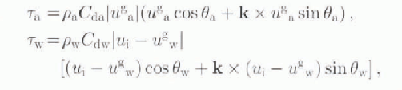
in which ρ a and ρ w are the air and water densities, C da and C dw the air- and water-drag coefficients, u g a and u g w the geostrophic wind and ocean current, u i the ice velocity, θ a and θ w the wind and water turning angles, and k a unit vector normal to the surface. Typical values for C da and C dw are 1.2 × 10⁻³ and 5.5 × 10⁻³, respectively. In the above equation for the wind-shear stress, the ice speed is considered small compared to the wind speed and is therefore omitted.
For the atmospheric case, various measurements made over the last 30 years yield drag coefficients ranging from 1 to 6 × 10⁻³, with more recent measurements being higher (Fig. 1). However, in most sea-ice modelling studies, a lower-range C da value of 1.2 × 10⁻³ is used instead (Reference HiblerHibler, 1979; Reference Flato and HiblerFlato and Hibler, 1992; Reference Holland, Mysak, Manak and OberhuberHolland and others, 1993). This choice is based on boundary-layer measurements made during the Arctic Ice Dynamics Joint Experiment (USA-Canada-Japan) (AIDJEX) project in 1972 (Fig. 1). The increasing trend with time in the measured drag coefficients is due to the measurements being made over increasingly rough surfaces and perhaps under increasingly unstable stratification conditions (Reference McPheeSmith, 1990).
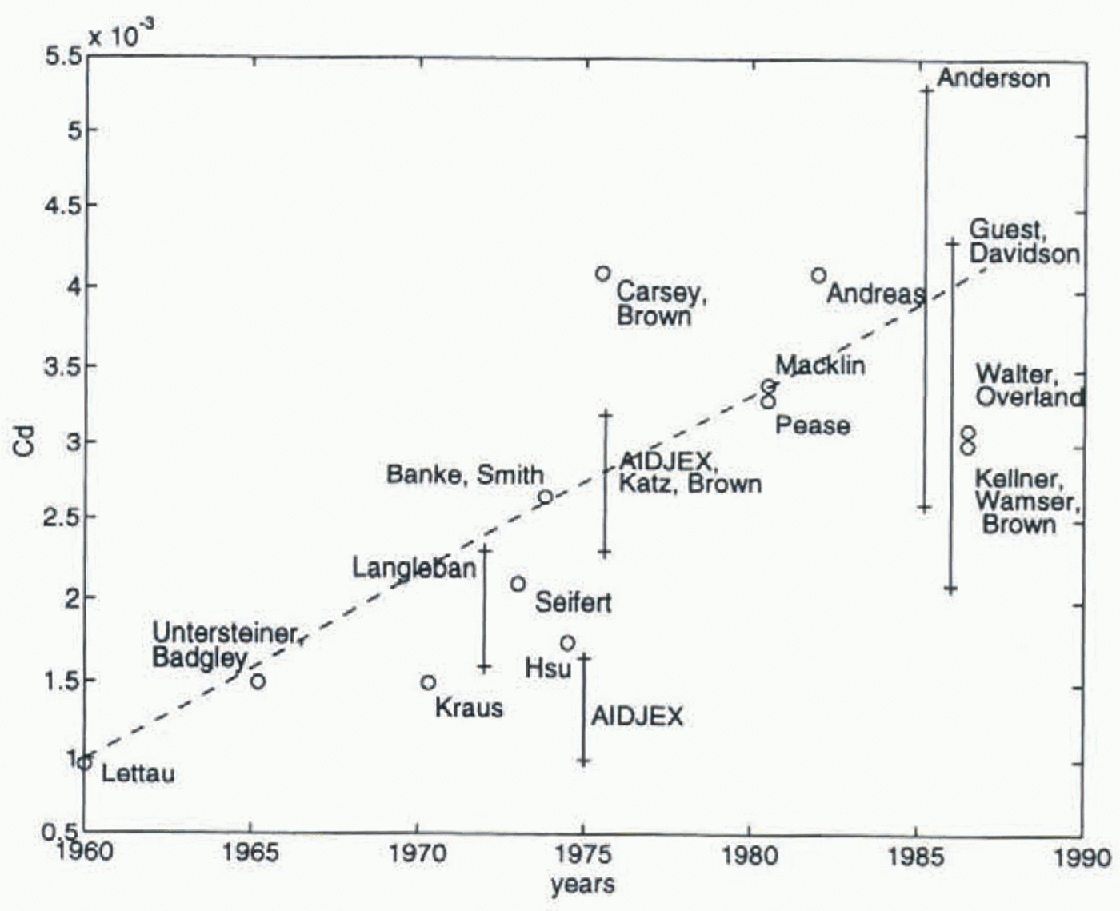
Fig. 1. Drug coefficients over ice from various experiments, reproduced from Reference SmithSmith (1990).
In this study, we attempt to include the effect of surface roughness in the dray parameterization; however, we ignore the influence of atmospheric stratification. To zeroth-order, we assume that sea-ice surface roughness is determined by ridging intensity. Since ridging results in the build-up of thicker ice, the sea-ice surface roughness is assumed to depend on ice thickness, Reference Stössel and ClaussenStössel and Claussen (1993) have also, among other factors, considered a dependence of the form drag on the ice-plus-snow freeboard. The relation between ice thickness and ridging intensity in the Arctic can be seen by comparing the observed ridging-frequency distribution (Fig. 2) with the measured ice-thickncss distribution in the Arctic (Fig. 3c). For the water–ice drag coefficient, the same dependence on surface roughness is assumed.
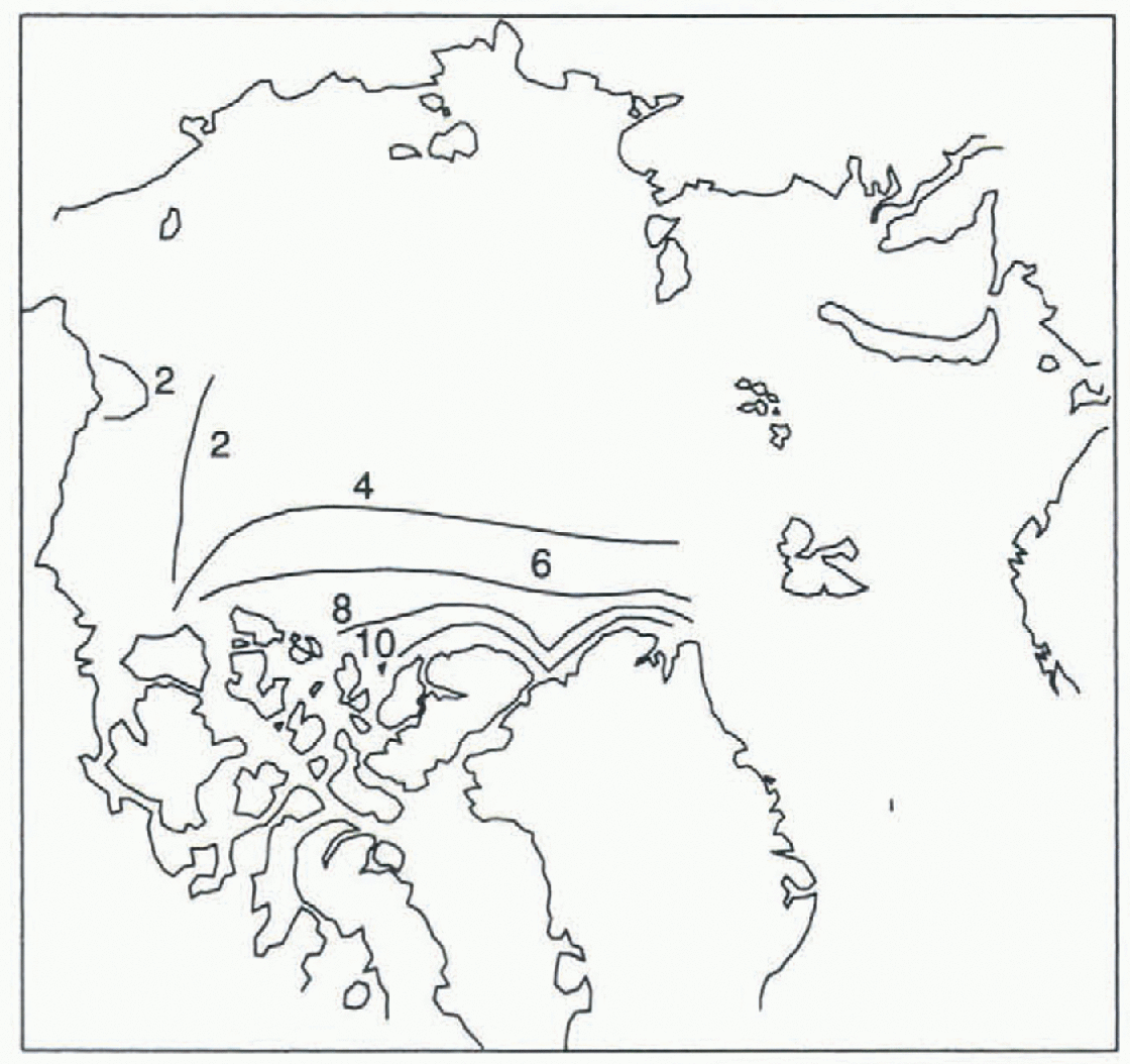
Fig. 2. Number of ridges (>1.22 m) km−1 in winter, reproduced from Reference Tucker and WesthallTacker and Westhall (1973).

Fig. 3. Simulated March ice-thickmss distribution with constant (a) and roughness-dependent (b) drag coefficient, and observed ice thickness from sonar data (c), in m. In (a) and (b), the ice edge is shown as a broad black line.
The lower range of measured drag coefficients (around 1 × 10⁻³) commonly used in large-scale sea-ice modelling studies are assumed characteristic of 1 m thick ice; the larger range values (around 5 × 10⁻³) are assumed to apply to 5 m thick ice (see Fig. 1). Inside those bounds, the drag coefficients are assumed to vary linearly with ice thickness: outside those bounds, the drag coefficients are specified to have these minimum or maximum values. Mathematically, this parameterization can be written as follows:
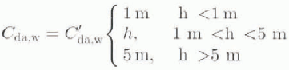
in which h is the sea-ice thickness, and Cʹda and Cʹdw the base drag coefficients taken as 1 × 10⁻³ and 5.5 × 10⁻³, respectively, The linear dependence of C dw on ice thickness h also allows the momentum and continuity equations to be written in terms of the ice flux u i h, which permits the use of more correct boundary conditions (i.e. no normal flux of ice at a solid boundary).
Results
Results from a 10 year simulation of the sea-ice cover in the Arctic Ocean and surrounding seas are presented in this section. A cartesian mesh with a grid resolution of 111 km is used on a polar stereographic projection of the physical domain. At high latitudes, the variation of the Coriolis parameter with latitude is small, and the f-plane approximation is used. The model is forced with the prescribed 19615 day running mean of the daily geostrophic winds with its yearly mean replaced by the 1954–89 annual climatology obtained from the National Meteorological Center (NMC) sea-level pressure analysis (Reference Flato and HiblerFlato and Hibler, 1992). This provides winds representative of climatology with realistic weekly variability. There is no particular reason for choosing the year 1961, except that it was not an anomalous year in term of sea-ice circulation (as were 1969 and 1984). Spatially varying, but steady, ocean currents were calculated from a single-layer reduced gravity model, appropriate for large-scale flows where the acceleration term in the momenturn equation is ignored (friction is represented using a linear drag law, and the normal velocity component is specified at open boundaries). In the Bering Strait, the normal velocity was set to obtain a constant inflow of 1 s.v. into the Arctic. The inflow- and outflow-velocity field in the North Atlantic was specified from Levitus sea-surface elevation data and scaled in such a way as to obtain no accumulation of water in the Arctic domain. Finally, solar forcing is the daily average value corrected for an 80% cloud cover (Reference LaevastuLaevastu, 1960).
The boundary conditions for the ice dynamic equations are zero normal and langential velocity at a solid boundary, and free outflow at an open boundary (Reference HiblerHibler, 1979). For the sea-ice thermodynamic equation, atmospheric temperature is specified from monthly climatology. The temperature at a given day is calculated as a weighted average of the mid-month climatological values. These temperatures w ere calculated from the (NMC) 850 mb height and temperature fields, assuming a linear temperature profile between the 1013 and 850 mb levels. For the ocean, the temperatures at open boundaries are specified from monthly climatologies extracted from the Lcvitus (1994) data. At continental boundaries, the ocean heat flux is considered to be zero (a continent is regarded as a perfect insulator).
The model was integrated for 10 years to reach a stable seasonal cycle using a 1 day time-step. To isolate the effects oi the drag-law parameterization on the simulated thickness-distribution fields, the same ocean currents and atmospheric temperature fields are used in the simulations. The results shown are the simulated winter climatological thickness distributions using a constant- and a thickness-dependent drag coefficient. The model results are compared with sonar data for ice thickness.
March ice thickness and ice-edge position
Figure 3a shows the simulated winter climatological thickness distributions in the Arctic using a constant drag coefficient, which can be compared with the sonar measurements (Fig. 3c) reported by Reference Bourke and GarrettBourke and Garrett (1987). The ice-edge position, defined as the 5-tenth ice-concentration contour, is also included in these figures. The model contour-line patterns reproduce the observations reasonably well, with ice thickness ranging from 1 m near Asia, to 7 m north of Greenland. In the Laptev and East Siberian Seas, the simulated ice thickness (2–3m) is larger than observed (<1 m). The modelled ice-free region in the North Atlantic cxlends over the whole of the Norwegian and Barents seas due to the advection of warm water by the Norwegian Current. In the winter, whether the Bering Strait is open or closed has a strong influence on the ice-thickness distribution in the Chukchi Sea. When open, the resulting ocean current pattern produces significantly thicker ice north of the Bering Strait. However, the temperature of the water entering the domain is very close to freezing point, and thus does not have a significant influence on the growth of ice in this region. In the Barents Sea, the ice margin is very well reproduced; however, in the Greenland Sea the ice edge is too far east. This is due to prescribed ocean currents that have a weak recirculation of water in the Greenland Sea.
Figure 3b shows the simulated mid-March thickness distribution in the Arctic using the roughness-dependent drag coefficient as described in the previous section. In this simulation, ice thickness ranges from 1 to 7 m, as before. However, now the ice-thickncss spatial distribution poleward of the northern Canadian islands is significantly different and is in better agreement with the observations. In this region, the ridging activity is high and the ice is assumed to be rough; this results not only in a higher wind stress, but also in ice drift following the wind more closely (the ratio of water drag to the Coriolis effect is higher). Both of these effects contribute to a higher ice build-up against the western part of the northern Canadian coast, as observed in the thickness field (Fig. 3c). In thinner ice regions the roughness-dependent drag coefficients approach the minimum value and little difference in the thickness distribution is found between the two models.
Conclusions
In the present study, ice-surface roughness is assumed to increase with ridging intensity, which in turn is responsible for ice thickening. Consequently, the drag coefficients are considered proportional to ice thickness. The effects of atmospheric stability on the air–ice momentum transfer, however, is not considered.
A long-term integration of the sea-ice model with both a constant- and roughness-dependent drag coefficient yield a range in ice thickness that is in agreement with ice observations. However, the ice-thickness spatial distribution in the Canada Basin for the two simulations is significantly different. The results using a constant drag coefficient yield a more uniform thickness build-up against the northern Canadian islands, whereas the results using the roughness-dependent drag coefficient results in an offshore tonguc of thicker ice in the western Arctic; this is in better agreement with thickness observations. In general, the simulations show that spatially varying drag coefficients, within the range of observed values, have a strong influence on the calculated ice-thickness distribution, and an attempt to incorporate this effect into sea-ice modelling studies is desirable.
Acknowledgements
B. Tremblay is grateful to NSERC and FCAR, and L. A. Mysak to AES and NSERC for financial support during the course of this work.


