


Introduction
This paper is based mainly on field work conducted during the Norwegian Antarctic Expedition (NARE) 1978-79. Some iceberg statistics are also included from NARE 1976-77. Both expeditions operated in the South Atlantic-Weddell Sea region, using the small Norwegian icebreaker/sealer Polarsirkel, and were organized and led by Norsk Polarinstitutt (Figs. 1 and 2). The 1978-79 expedition also carried two Bell 206B (Jetranger) helicopters, which enabled landings to be made on 24 icebergs (Fig. 3). The studies carried out on these icebergs are listed in Table I.

Fig.1. Polarsirkel at the ice front of Riiser-Larsenisen. Photo: Børre Johansen.

Fig.2. Cruise tracks of NARE 1976-77 and 1978-79.

Fig.3. Location of icebergs visited during NARE 1978-79.
Table I Research on Icebergs During Nare 1978-79.
(R-E is radio echo-sounding, PRT-5 is precision radiation thermometer, SSS is side-scan sonar, CTD is conductivity-temperature-density.)

The iceberg studies were a small part of the total research of the expedition, which involved 35 scientists. Other programmes had first priority in the use of the ship, so most iceberg flights were made while the ship was involved with these. When a suitable iceberg was sighted, from the ship or from the air, a group would be flown to work on it, supported by flights with radio echo-sounding equipment and PRT-5 radiometer. In the meantime, the ship would continue with other programmes, usually travelling at speeds of 5 to 12 knots. Normally, this permitted two or three hours’ work to be carried out on the iceberg, which was adequate for executing most of the programmes listed in Table I. However, considerably longer periods were spent on icebergs nos. 7, 20, and 22 in order to complete the programmes. Altogether 14 scientists and technicians were involved in iceberg research during 1978-79. In addition to the 24 icebergs listed in Table I, a few others were visited briefly. Radio echo-sounding flights were made over nine bergs, and radiometric measurements made on eleven. Automatic instrument stations transmitting over the N0AA-N/ARGOS satellite system were placed on eight bergs. In all, 2 119 icebergs were observed from Polarsirkel and classified according to size and other properties, and, in addition, 528 icebergs were classified during seven helicopter surveys. Also included are 2 623 icebergs which were counted on NARE 1976-77, giving statistics on a total of 5 270 icebergs. Other results of the NARE iceberg studies are given in Foldvik and others (1980 [a], [b], and [c]), Reference Klepsvik and FossumKlepsvik and Fossum (1980), and Reference VinjeVinje (1980).
Stratigraphy, Density, and Mass Balance
In the absence of any other information, it has been assumed that a tabular iceberg has the same properties as the ice shelf from which it calved (Reference Weeks, Mellor and HusseinyWeeks and Mellor 1978). Our measurements show that this concept must be modified, even in the case of an iceberg close to the Antarctic continent, because an iceberg experiences above-freezing temperatures and melt-water percolation.
Shallow pits, usually between one and two metres deep, were dug on 11 icebergs. In addition, ice cores of a maximum length of 6.5 m were collected from three bergs. The stratigraphy revealed considerably more ice layers than are found on neighbouring ice shelves (Reference SchyttSchytt 1958). The proportion of ice layers in the pits varied between 6 and 40%, with an average of 14%. In addition, the upper one or two metres of some icebergs consisted of near-solid ice, so that no pits could be dug. However, drilling on these icebergs revealed layers of looser firn underneath the compact ice.
The stratigraphy of six icebergs consisted of thin ice layers and depth hoar, which were classified as surfaces of the 1976-77 and 1978-79 summer seasons. The average annual surface net balance for these bergs was 0.26 m water equivalent, with a range of 0.12 to 0.41 m. However, the net balance of bergs where the upper 2 m consisted of ice was probably negative or near-zero during recent years. Thus, on the whole, the icebergs have less positive mass balance than the nearby ice shelves, which are quoted at about 0.5 m (Reference SwithinbankSwithinbank 1957, Reference LundeLunde 1961). The main reason for this difference is deflation. Probably the annual surface net balance of most icebergs visited was between +0.2 and -0.2 m.
The above data all refer to icebergs south of 69°S. One iceberg was visited near Bouvetøya, at 54°S. Here the snow was very wet and had low bearing strength down to 1.8 m depth, where ice was encountered (N. Nergaard, personal communication). This iceberg had drifted for several months in the open sea with air temperatures of about 0°C, and percolating melt water and rain had raised the temperature of the snow and firn, at an unknown depth, to melting point. No density measurements were made on the iceberg off Bouvetøya. Near-surface measurements of five icebergs south of 69°S. showed consistently higher densities than those reported from neighbouring ice shelves (Reference SchyttSchytt 1958), with a difference usually between 100 and 150 kg m-3. However, no density measurements were made at a depth greater than 2.5 m.
Ice Temperatures and Heat Flow
Temperatures were measured on six icebergs by means of thermistor chains. Measurements were generally made at three or four levels with maximum depths ranging from 4 to 10 m (Table I). As most measurements cover periods of one or two hours there may be errors due to residual drift. However, it is likely that errors are less than 1°C . All temperature profiles were obtained in February and all had similar shapes, with gradients ranging from 1.0 to 1.6°C m-1. Maximum range of temperature at any depth was 5°C. Figure 4 shows a combined curve averaged from all measurements, and a comparison with the ice-shelf data from Maudheim at 71°S., 11 °W. (Reference SchyttSchytt 1960) and from Norway station at 70°30’S., 2°30’W . (Reference LundeLunde 1965).

Fig.4. Temperature measurements on icebergs and ice shelves.
The stratigraphy, density, and temperature data show that the icebergs differ from the ice shelves in one important feature: the percolation and refreezing of water in the snow and firn. The ice layers indicate an average annual refreezing of 0.03 to 0.04 m and similar values are suggested by the density data. The heat released by this refreezing would be adequate to raise the temperature of an annual snow layer of 0.5 m thickness more than 25°C, i.e. to the melting point.
Figure 4 shows that the mean temperature in the upper 10 m of the icebergs is about 6° higher than for the ice shelves. There are three main reasons why the temperature is not increased by the larger value corresponding to the annual refreezing: the heat flow to the firn below, the larger heat loss in winter from the icebergs because of warmer near-surface temperatures, and refreezing of melt water may have been in effect for only a few years. If data were available on the ice-shelf properties at the time of calving, and on the climate around the iceberg, then heat flow to the berg could be modelled. This would enable the time since the iceberg calved to be estimated.
The observations on the iceberg off Bouvetøya support the idea that once an iceberg drifts northwards into the west wind drift, its surface layers will rapidly warm to 0°C. Melt water and rain will percolate through the firn even if extensive ice layers develop. Although pockets of colder firn may remain it will not take long for the permeable part of the iceberg to reach the melting point. For example, a 225 m-thick iceberg with a freeboard of 36 m will have the firn/ice transition at about sea-level. If the internal temperature of the berg is -17°C, then the refreezing of about 2 800 mm of water is needed to warm the upper 36 m to the melting point. For an iceberg in the open sea it would probably take less than one year for the combined effects of surface melt, rain water, sea spray, and condensation to add this amount of liquid water and so to bring the permeable part of the iceberg to the melting point.
Thickness and Shape of Icebergs
Radio echo-sounding of nine bergs was carried out, using a Scott Polar Research Institute Mark IV echo-sounder, fitted with a Honeywell oscillograph recorder. The equipment was mounted inside the Jetranger helicopter, leaving sufficient room for a technician and a navigator in addition to the pilot. A 3.8 m antenna was provided by the Technical University of Denmark, and was mounted, using fibreglass supports, alongside the helicopter at a distance of 2 m.
Most icebergs were profiled in one flight along the long axis and two flights across the berg at an elevation of 30 to 50 m above the surface. The sections were then repeated at about 400 m elevation. For seven of the icebergs the records were good to fair and yielded fairly reliable thickness values. For one iceberg the record was mediocre, and one record was poor. An example of a good record is given in Figure 5.

Fig.5. Radio echo-sounding of iceberg no. 13. Both records have the same horizontal and vertical scales. The iceberg is 300 m thick. The profiles were flown about 30 m above the iceberg, so the surface return was masked by the outgoing signal. Both records show the base of the iceberg and (in some places) a double echo from the base.
The results of all the echo-soundings are shown in Figure 6. The icebergs have commonly an arched cross-section from the time of formation, because the ice shelf fractured along depressions or zones of thinner ice which represent zones of weakness (Fig. 7). However, the icebergs show less under-water arching than expected from the above-water shapes if the bergs were in isostatic equilibrium at all points. Thus there are internal stresses set up by the arching in addition to the disequilibrium at the free faces described by Reference ReehReeh (1968).

Fig.6. Iceberg thicknesses measured by radio echo-sounding. ̅H is mean thickness. Δ is difference between maximum and minimum thickness.

Fig.7. Undulations are common near ice fronts as here in Dronning Maud Land at 27° E. Photo by Lars Christensen’s expedition 1936-37 (copyright Norsk Polarinstitutt).
surface crevassing parallel to the free faces was generally observed, usually with orthogonal crevasse patterns at the corners of the bergs. The frequency of surface crevasses decreases with distance from the edge, and, on many of the bergs, crevasses were not seen at distances of more than 100 m from the edges.
Although the radio echo-sounding clearly showed bottom crevasses on nearby ice shelves (Fig. 8) no bottom crevasses were observed on any of the icebergs. The reason for this may be that the icebergs studied were unusually free of faults and bottom crevasses.

Fig.8. Radio echo-sounding records from the central part of Riiser-Larsenisen, showing numerous bottom crevasses.
The iceberg thicknesses measured by radio echo-sounding varied between 200 and 340 m. From this a density curve was constructed which gives the best fit between freeboard and thickness. The curve is based on the assumption that the submerged iceberg walls are vertical and the bottom is flat. The upper few metres of the iceberg density curve are 100 to 150 kg m3 higher than for the ice shelf at Maudheim (Reference SchyttSchytt 1958), but below this the two curves asymptotically approach one another, reaching 917 kg m-3 at 200 m depth. The iceberg density curve was used to calculate the relationship between freeboard and thickness for an “average” berg and the results are shown in Figure 9. Although these curves probably represent real icebergs better than corresponding curves based on ice-shelf data (Reference Weeks, Mellor and HusseinyWeeks and Mellor 1978) it must be Stressed that the observed thicknesses show deviations of up to 18 m from those determined from the computed average thickness/freeboard curve. Although these variations may be partly caused by varying density profiles it seems more likely that the main cause is incorrect assumption of the underwater shape. The observations of Reference Klepsvik and FossumKlepsvik and Fossum (1980) indicate that the walls may not be vertical, and our observations of arching suggest that the base may not be a plane.

Fig. 9. Relationship between freeboard and thickness for the icebergs generalized from the observed freeboards and ice thicknesses.
Blasting Experiment
Obviously the danger of calving means that the edge of an iceberg is not the safest place to work. However, the likelihood of calving may be estimated from the degree of under-cutting and the frequency of crevassing, thus allowing visits near to the edge under suitable circumstances and with safeguards (Fig. 10). Five holes of 0.05 m diameter were drilled to a depth of 6 m in a line approximately parallel to the edge, and at a distance of between 3 and 8 m from the free face, and with 5 m between them. Each hole was filled with 30 kg of explosive (TNT), and the resulting blast yielded a clean cut except for one hole that crossed a crevasse and “leaked”. About 500 m3 was blasted off, giving a yield of 3.3 m3/kg TNT.

Fig.10. Personnel drilling holes for the blasting experiment near the edge of iceberg no. 22.
Iceberg Statistics
Figure 11 shows the size distribution for 2 119 icebergs observed during NARE 1978-79. Most icebergs were observed from the ship, and at a distance, so that only one horizontal dimension was recorded and used for statistical purposes. When both horizontal dimensions were recorded the shortest has been used. However, the size distribution in Figure 11 does not change significantly when the length is substituted for the width. The important feature of this size distribution is that the number of icebergs increases with decreasing size. This implies that, in addition to minor calving around the edges, splitting must be an important process.
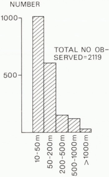
Fig.11. Size distribution of observed icebergs.
The observed size distribution differs markedly from those based on earlier field observations which have implied approximately equal numbers of icebergs in each class of size and have therefore suggested that attrition is the dominant process of iceberg breakdown. These include Reference RomanovRomanov (1973) with 720 observations, Reference GordiyenkoGordiyenko (1960) with 397 observations (stated in Reference NeshybaNeshyba 1980), Reference NazarovNazarov (1962) with 407 observations, and Reference Dmitrash ZhDmitrash (1965) with 139 observations, totalling 1 663. These were mostly around east Antarctica and it is possible that there are differences in size between icebergs of that region and of the present study area in the Weddell Sea and off western Dronning Maud Land. However, the explanation may be that the earlier statistics do not describe the total iceberg population. They include observations from any ships over many seasons, yet the number of observations is smaller than the number of observations made in each of the two NARE seasons. The earlier published statistics probably represent the size distribution of large icebergs only; the smaller bergs have generally not been included. Unless the observer has very strict instructions to include all icebergs there will be a tendency to record only the large bergs; smaller ones in the same area may be ignored or missed.
The earlier statistics have been used to make some conclusions on iceberg melt rates and breakdown processes. It would now appear that these are unreliable. Reference NeshybaNeshyba (1980) seems to have recognized that they record the small icebergs inadequately.
Size distributions based on Landsat-1 imagery have been published by Reference Hult, Ostrander, Freden, Mcrcanti and BeckerHult and Ostrander (1974). They give data on 672 icebergs within the fast ice and pack ice of the Bellingshausen Sea, and 74 at the edge of the pack ice. The size distributions of the two groups were markedly different, with a larger mean and a lack of small icebergs for the group near the coast. Again, these statistics may not describe a typical iceberg population. One obvious source of error was the limited resolution of the Landsat imagery, which, for Landsat-1, was about 100 m. Small icebergs were therefore not observed. But there is another problem which was not remarked on when their data were recalculated by Reference Weeks, Mellor and HusseinyWeeks and Mellor (1978). Hult and Ostrander’s data are based on clusters of icebergs observed in eight images. Two-thirds of the 672 icebergs seen near the coast were from the area off the highly active Thwaites Glacier; more than half of these were in the complex fast-ice/iceberg/ice-shelf zone between Thwaites Glacier and Bear Peninsula. These had in fact not yet become true icebergs and may later become part of an ice shelf in the manner known to occur in the area north-east of Hal ley Bay (Reference ThomasThomas 1973). This is an atypical situation, and measured sizes of the icebergs from this area cannot be taken to be representative of average Antarctic icebergs.
Figure 12 shows the relation between length and width of the 24 icebergs that were landed on and studied in detail during NARF. 1978-79. The ratio length/width varies between 1:1 and 4:1, averaging 1.6:1, which is the same as the value quoted by Reference Dmitrash ZhDmitrash (1973). There is no correlation between freeboard and horizontal dimensions, that is to say there is no reason to expect an iceberg with large horizontal dimension to be especially thick.

Fig.12. Relationship between length and width of the icebergs visited.
Figure 13 shows numbers of icebergs encountered on the crossings to and from Antarctica on Polarsirkel, plotted against distance from the coast. There is strong evidence that the number of icebergs does not decrease regularly with distance from the coast as suggested by statistics which have been used to derive melt rates. Rather, the number is uniformly higher in the east wind drift. Then there is a zone of very few icebergs and little current, followed by an increasing number in the Antarctic Circumpolar Current. This picture will be different in other areas around Antarctica depending on the regional circulation. For the area of this investigation it is clear that flow into the central area of the gyre, and therefore the number of icebergs there, is very low. The variations in distribution pattern with time should be noted. Large numbers of icebergs were encountered each season in January, whereas the number was very much smaller in March. This suggests that many ice-bergs do not survive two months in the open sea. Figure 14 shows the distribution by size; this again emphasizes the absence of icebergs in the zone about 700 km from the coast in the central area of the Weddell gyre. This confirms the evidence from iceberg drift (Reference TcherniaTchernia 1974, Reference VinjeVinje 1980). Figure 15 demonstrates further the evidence for rapid destruction in open water. The solid part of the circles represents the proportion of icebergs that have not been overturned, and the proportion of such bergs drops very rapidly with increasing distance from the coast. However, there are also numerous observations of larger bergs, including those monitored by the Norwegian automatic buoys, that survive for long periods in open water. The paradox is resolved if it is accepted that those icebergs that contain flaws will probably break up fairly rapidly under the action of waves and swell, but those that have fewer internal weaknesses and survive this initial filtering have the potential for surviving for at least one to two years in the open sea. Thus, icebergs that have survived a season in the open sea are likely to be fairly free of faults, and it seems that the radio echo-sounding was carried out on this kind of iceberg. Icebergs for towing should be selected from the group that has proved its resistance to fracturing by surviving for months in the open sea. It is reasonable to expect that different ice shelves produce icebergs with different degrees of internal weakness, depending on the flow and stress history of the ice shelf and the inland ice.

Fig.13. Number of icebergs encountered on crossings to and from Antarctica.

Fig.14. Relationship between size distribution and distance from Antarctica of observed icebergs.

Fig.15. Proportion of overturned or small icebergs encountered at various localities during NARE 1978-79.
Table II. Thickness, Mean Density, and Density at Sea-Level for Selected Freeboards, Based On Same Relationship as Figure 9

Acknowledgements
This work would not have been possible without the enthusiastic cooperation of many of my colleagues on NARE 1978-79, especially Kjell Nythun, who had the technical responsibility for the radio echo-sounding, and Bjørn Wold, who worked on the icebergs. I am also grateful to colleagues at Norsk Polarinstitutt for critical comments, in particular Torgny Vinje for many helpful discussions and Øivind Finnekåsa, who did the computer processing. “Icebergs for the Future” of Paris provided support for the radio echo-sounding programmes, and partial support for some of the other studies, for which I express appreciation.


