


1. Introduction
Increased human activity in mountain regions, deforestation from pollution, forestry and increased number of ski resorts, as well as a generally reduced societal acceptance of risk, have caused a growing demand for hazard zoning and avalanche protective measures. Enjoined building regulations and the increased economic consequences of hazard zoning further imply an increasing demand for risk quantification including quantification of the uncertainty of the estimates. This is a great challenge, especially in potential avalanche terrain where there are few observations of snow avalanches, where old buildings are present in the potential run-out zone, and where the local climate does not favour severe snow accumulation.
According to the Norwegian building regulations, the “safe” areas in the snow-avalanche-prone regions of Norway are those areas where the nominal annual probability of a house being hit by an avalanche is <10–3 The term “nominal” implies that the probability cannot be exactly quantified and reflects the uncertainty of the estimates. Alternatively, safety can be linked to impact pressure (Reference Salm, Burkard and GublerSalm and others, 1990; Reference McClung and SchaererMcClung and Schaerer, 1993) and to vulnerability and survival probability (Reference Keylock, McClung and MagnussonKeylock and others, 1999; Reference Jonasson, Sigurdsson and ArnaldsJonasson and others, 2000; Keylock and Barbolini, in press).
In practice, the avalanche expert estimates contour lines of specific annual probabilities, based on the local climatic conditions, topography and knowledge of the average frequency of avalanche occurrence, in combination with statistical and/or dynamics models for prediction of run-out distance, velocity and impact pressure.
Various statistical models for run-out distance calculations based on the terrain profile have been presented (Reference Lied and BakkehaiLied and Bakkehoi, 1980; Reference Bakkehai, Domaas and LiedBakkehoi and others, 1983; Reference McClung and LiedMcClung and Lied, 1987; Reference McClung and MearsMcClung and Mears, 1991). Reference Keylock, McClung and MagnussonKeylock and others (1999) also take into account the interaction of variable avalanche width and differences in avalanche trajectory. Section 2 presents the statistical/topographical α/(β model (Reference Lied and BakkehaiLied and Bakkehoi, 1980; Reference Bakkehai, Domaas and LiedBakkehoi and others, 1983) applied in this paper for run-out distance calculations. Such models return a conditional probability distribution of extreme run-out distance, given that a major avalanche occurs. To obtain the unconditional annual probability distribution, one needs also to estimate the annual probability of release of an avalanche. Hence, the “actual” annual probability is the run-out exceedance probability computed from statistical/topographical models times the annual probability of avalanche release in a given area.
Mechanical models for avalanche release based on a strength-to-load ratio have been presented by, for example, Reference PerlaPerla (1975), Reference SommerfeldSommerfeld (1980), Reference FohnFohn (1987), Reference McClungMcClung (1987) and Reference McClung and SchweizerMcClung and Schweizer (1999). In section 3.1, models based on the mechanics of slab avalanches and structural reliability methods or Monte Carlo simulations are applied as a basis for calculating the annual probability of avalanche release. A probabilistic approach was presented by Reference Conway and AbrahamsonConway and Abrahamson (1988). In section 3.2 an alternative statistical model based on observations is presented.
Section 4 explains how statistical/topographical run-out models can be combined with release probability models in hazard zoning. Alternatively, the run-out distance may be calculated by integrating statistical and dynamics models (Reference Barbolini, Gruber, Keylock, Naaim and SaviBarbolini and others, 2000), or combining simple and more advanced models (Reference Harbitz, Issler, Keylock and HestnesHarbitz and others, 1998), and hence reducing the subset of permissible parameter values to a tolerable level. Reference BarboliniBarbolini (1999) evaluates the uncertainty of model results further, and discusses probability distribution functions for the input parameters of the release and dynamics models.
Some recommendations for future hazard zoning procedures are included in the conclusions.
2. Extreme Run-Out Distance Prediction
2.1. Statistical/topographical model
The statistical α/β model (Reference Lied and BakkehaiLied and Bakkehoi, 1980; Reference Bakkehai, Domaas and LiedBakkehoi and others, 1983) predicts the extreme run-out distance for a snow avalanche solely as a function of topography. The run-outdistance equations are found by regression analysis, correlating the longest registered run-out distance from 206 Norwegian avalanche paths to a selection of topographic parameters. The parameters that have proved to be most significant are presented in Figure 1.

Fig. 1. Topographic parameters describing terrain profile.
The average inclination of the avalanche path between the starting point and the point of 10° inclination along the path profile, 0, is empirically found to be the best characterization of the track inclination. The regression analysis revealed that the 0 angle is also the most important topographic parameter. In fact, it appears that, in general, 0 is the only statistically significant terrain parameter. A 0 point is accepted only if it is inside the section of the profile where the angle between the tangent of the best-fit parabola at the 0 point and the horizontal plane is 5–15°. The model is most appropriate for analysis along longitudinally concave profiles. The run-out distance is represented by the average inclination of the total avalanche path, a.
The calculated run-out distances are those that might be expected under snow conditions favouring the longest run-out distances. The assumption of small variations in the physical snow parameters giving the longest run-out distance is only valid within one climatic region.
The usual form of the α/β model for a random a value is a = a0 + b + W, where a and b are regression parameters and W is a normal N(0,σ) variable. Based on 206 (a, 0) observations, the estimated values for the unknown parameters are a* = 0.96, b* = –1.4° and standard deviation a* = 2.3° (where * is used as a general superscript for an estimator), i.e.
The empirical correlation coefficient between the observed a and 0 values is 0.92. No apparent deviation from the standard assumptions of independent residuals with constant variance independent of β is seen from residual plots (the residuals are the difference between observed a values and the a value from the fitted regression line at the 0 values corresponding to the a observations). However, the frequency histogram of the residuals indicates a skew distribution with the heaviest tail towards small a values. This raises the question whether the assumption of a normal residual distribution is correct. Regardless of residual distribution, the angle 0 must be within the range where the model is reasonable. In addition, the number of observations is assumed to be large enough for the uncertainty of the regression line itself and the uncertainty of the standard deviation of W, a, to be negligible.
The appropriate interpretation of the α/β model with respect to hazard zoning is not obvious. This is partly due to the fact that mostly there is only one a observation recorded for each path, and partly due to the scarcity of knowledge about the actual observation period and the number of avalanches that have occurred. It is therefore difficult to know if, for example, a reflects the variation of possible a values for each specific path, or if a reflects the variation among paths due to topographical or other reasons. These two alternatives are further discussed in sections 2.2 and 2.3.
Based on an analysis of 45 Icelandic events, Reference Johannesson and HestnesJohannesson (1998) found that the intercept term is statistically insignificant, and that the equation without intercept for a modified and trimmed dataset of 192 Norwegian events reads a = 0.93/3 with standard deviation of 2.1°. Even though the latter equation is mathematically simpler, it was decided to apply the more general and well-known Equation (1) in this context. A more complete description of the α/β model is presented by Reference HarbitzHarbitz (1998).
2.2. Extreme-value model
If the observed a value is the most extreme run-out angle for N avalanches, αi,…,αN, that have occurred in one single path, then the assumption of a normal W distribution is not realistic. In this case the Gumbel distribution is an actual extreme-value distribution for W for sufficiently large N. Let / denote the distribution of the individual a values αu…,αN. The Gumbel distribution is the appropriate asymptotic extreme value distribution for a range of different f’s, among them the normal distribution (Reference GalambosGalambos, 1978). A consequence of such an extreme-value interpretation is that the regression line is dependent on N, which increases with observation period and conditions favouring avalanches.
Assume that the actual (a, 0) observations are based on an average observation period of 100 years, and that the number of avalanches behind each extreme a observation does not vary too much. In this case the fitted regression line is a ”100 year” line predicting the lowest a value during a 100 year period.
A nice feature of the Gumbel distribution is that once the regression line for a given period (e.g. 100 years) is established, the corresponding line for any other period can easily be found. By a change from a 100 year line to a 1000 year line, for example, the Gumbel distribution gives a recipe which quantifies how much the regression line is to be lowered (section 4).
2.3. Single-value model
If the observed a value is due to only one single avalanche that has occurred in each path during the observation period, the assumed normal distribution is only one of several candidates. In this case, the regression line is stationary and the effect of an increased number of paths with a observations is that the estimation of the unknown parameters a, β and a is improved. The W distribution (e.g. N(0, σ)) is now the fundamental distribution used to find a criterion for hazard zones.
As an example, assume that a safe a value for a specific path corresponds to the lower 10 percentile in the W distribution. If a reflects the variation of possible a values for the specific path, this is equivalent to assuming that the actual a value belongs to the ”10% most extreme potential avalanches in the specific path”. If, on the other hand, a reflects the variation among paths due to topographical or other reasons, this is then equivalent to assuming that the specific path belongs to the “worst 10% cases” (i.e. longest run-out) among paths with the same /3 value. For practical use, there is no difference between these two interpretations of a.
3. Probability of Release
3.1. Mechanical probabilistic model
General background
Field observations and measurements show that the physical mechanism governing the release of a slab avalanche can vary greatly depending on the character of the deformation in the weak layer or interface beneath the slab where the slide initiates (Reference McClungMcClung, 1987). The initiation of a slab avalanche is a multi-phase and progressive fracture process. Referring to Figure 2, the following stages of a snow-slab avalanche fracture are to be considered:
Shear fracture along the shear interface, which is more-or-less parallel to the surface.
Tensile fracture at the crown of the snow-slab avalanche.
Flank fracture at the sides of the slab.
Compressive fracture at the stauchwall (lower limit of the release zone).

Fig. 2. Snow-slab avalanche definitions, coordinate system and acting forces. From Reference LackingerLackinger (1989).
A common practice is to investigate the slab stability solely with respect to shear fracture in the shear interface, disregarding the boundary conditions along the entire snow-slab area, as well as the fracture’s progressive character. A strength-to-load ratio (safety factor in the geotechnical sense) is defined as the ratio of the shear strength along the potential failure plane and the driving shear stress parallel to the slope surface. The strength-to-load method has often proved unsatisfactory. Therefore, in the mechanical model described below, the boundary conditions along the entire snow-slab area are considered. Progressive fracture as described by Reference SalmSalm (1986) is beyond the scope of this paper.
The ’standard” snow-slab avalanche
The following forces act on the “standard avalanche” shown in Figure 2: T is the driving component of the total weight W of the release slab, FT is the tension force at the crown, FC is the compression force at the stauchwall, FF is the flank force and Fs is the shear force along the shear surface. These forces can be estimated from the following equations:
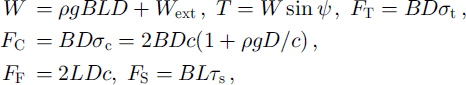
where p is the density of the snow, g is the gravitational force per unit mass, B, L and D are the width, length and thickness (perpendicular to the surface) of the slab, respectively, Wext is the external load on the slab (e.g. skiers, snowmobile, etc.), V is the slope inclination, σt is the tensile strength of the snow, σc = 2c(1 +ρgD/c) is the compressive strength for the stauchwall, c is the shear strength of the snow slab, and τs is the shear strength of the shear surface. The relationship between σc and c is obtained from the passive earth pressure theory for cohesive material.
A safety factor may be defined as the ratio of the total resisting forces in the downslope direction to the driving shear force:
According to Reference Perla and ColbeckPerla (1980), the “standard avalanche” is characterized by the following values: p = 220 kg m–3, B = 50 m, L = 50 m, D = 0.7 m and ψ = 38°. Reference LackingerLackinger (1989) performed a parametric study of the “standard” snow-slab avalanche using the ranges of strengths presented in Table 1.
Table 1. Ranges of strengths for parametric study of the “standard”snow-slab avalanche

With the minimum values of all strength parameters, the evaluated safety factor is only 0.72, whereas using the maximum values results in a safety factor of 6.09. The range of the safety factor clearly shows the practical problem one is faced with in a deterministic approach. When there is large uncertainty in the actual value of important parameters, a probabilistic approach capable of accounting for the uncertainties is called for. A probabilistic model for “standard” snow-slab avalanche is described below.
First-order reliability method (FORM) approximation
Equation (3) defined a safety factor SF with the property that SF < 1 implies a snow-slab avalanche release. Let
define a so-called limit state function where now g < 0 is synonymous with a snow-slab avalanche. X here denotes a vector of stochastic basic variables (e.g. the variables introduced in Equation (2) and Table 2).
Table 2. Probability distribution of basic random variables in the standard avalanche model

Let f(x) denote the joint probability density function of X. The probability of an avalanche occurring is then
i.e. the integral of f(x) over the domain Ω in x space where g < 0. In order to illustrate these concepts, imagine a huge number of “critical” situations to be examined by avalanche experts in order to assess the probability of avalanche occurrence. Assume that in each of these situations all the basic variables could be measured. These joint measurements could then be used to establish the unknown f(x). The integral above should then in principle give the same value as the proportion of the critical situations that caused an avalanche to occur.
In general, the p f integral cannot be solved analytically, partly due to the generally complicated boundary between the safe and non-safe domain in x space. FORM is an approximate method to calculate pf based on the following two steps:
-
1. The vector of basic random variables X is transformed into a vector Z of independent N(0, 1) variables by applying the Reference RosenblattRosenblatt (1952) transformation.
-
2. The transformed limit state function g(x(z)) is linearized at the point of maximum probability density, i.e. the point on the failure boundary closest to the origin in z space, which is found by numerical searching algorithms.
The linearization point, z*, is called the design point, and the distance from the origin to z* is called the reliability index, d (rather than the normal designation /3 to avoid confusion with the /3 angle above). It can be shown that the pf value found by this hyperplane approximation to the generally curved failure boundary is
which increases with decreasing d. Φ is the cumulative standard N(0,1) distribution function. The FORM approximation is justified by the fact that the linear approximation is best where the probability density is largest.
The directional cosines, δo (rather than the normal designation a to avoid confusion with the a angle above), of the vector z* are called the sensitivity factors, because they indicate the relative influence of each basic variable on the reliability index. Note that the sensitivity factors combine the sensitivity of the original deterministic limit state function with the variance of the variable.
If some of the basic variables are correlated, the so-called representative sensitivity factors, δr, are more appropriate than δo as indicators of influence on pf. These are defined as
where K is a normalizing constant so that
![]() the inverse cumulative standard N(0, 1) distribution function, and F{x*) is the value of the cumulative distribution function of xz
at the design point, z*. For uncorrelated variables 70 = 7 r.
the inverse cumulative standard N(0, 1) distribution function, and F{x*) is the value of the cumulative distribution function of xz
at the design point, z*. For uncorrelated variables 70 = 7 r.
Monte Carlo simulation
The FORM approach described above relies heavily on the ability to find the design point, z*, accurately, as well as on the assumption of a reasonable hyperplane approximation to the true failure boundary. In worst case with a very curved boundary at the design point, pf can be wrongly estimated by several orders of magnitude.
Monte Carlo simulation is a supplementary and very useful tool for estimating the unknown pf value, as well as examining if the design point found by FORM is reasonable. The simplest approach is to generate n random N(0, 1) variables, ZU …, Zn, one for each stochastic variable, Xi, in the mechanical model, then calculate the corresponding variable values for xi (by applying the inverse Rosenblatt transformation) and the corresponding safety factor SF and g(X) = SF – 1. If this procedure is repeated Nsim times, say, and N_ of these simulations give negative g(X) (i.e. an avalanche release), an unbiased pf estimator pp is given as:
Further, N– is binomially distributed Bino(Nsim,pf), so that N– = 100 is sufficient in most cases to obtain a relative accuracy of about 10%. This corresponds to a required number of Nsim = 100/p, simulations.
Monte Carlo simulation can also be applied to examine the accuracy of the reliability index, d, and the design point, z*, found by FORM, for example by restricting the sampling domain to an n-dimensional small hypersphere with origin at z*,
and with z*sim equal to the z corresponding to dsim.
If the simulations provide results similar to those of the FORM analysis, this is a good quality support to the latter. If not, one should be extra-careful in the interpretations of the FORM results. When the p f results deviate substantially (e.g. by one order of magnitude), the simulated pf value should be preferred.
In cases where pf is so small that the numerical effort by the described method becomes prohibitive, there are other efficient techniques available for obtaining reliable pf estimates. Trusting that a proper design point is found (by FORM), the sampling domain can be restricted to the non-safe area outside the n-dimensional hypersphere in Z space with centre in the origin (Reference HarbitzHarbitz, 1986). By applying an appropriate variable transformation of z it can be shown that the required number of simulations is reduced by a factor one to the probability mass outside the d sphere, the latter probability found from the chi-square distribution with n degrees of freedom (Reference HarbitzHarbitz, 1986).
Calculation example
The “standard” slab avalanche is used. Nine basic variables are defined with the probability distributions given inTable 2. The mean values and standard deviations are chosen such that most of the variables span a range in agreement with the values presented inTable 1.
A correlation coefficient pc(ln c, In σt) = 0.8 is assumed between ln c and ln σt (cohesive and tensile strengths). According to Reference McClungMcGlung (1987), there is a scale effect on the average shear resistance of the weakness plane such that larger areas tend to have a lower shear resistance. In order to model this, the negative correlation coefficients ρc (ln τs In B) = –0.5 and ρc(ln τs In L) = –0.5 are used.
FORM results:
Using the FORM method gives the reliability index d = 1.5302 and the probability of an avalanche occurring pf = Φ(d) = 0.0630. Representative sensitivity factors, δr, are illustrated in Figure 3, demonstrating that shear resistance and snow-slab dimensions (length and width) dominate the influence on pf. If the correlations between shear resistance and the snow-slab dimensions are removed, the d value is increased from 1.53 to 1.98, corresponding to a decrease of pf from 0.063 to 0.024.

Fig. 3. Representative sensitivity factors δr with sign indicating direction of influence on d.
Monte Carlo simulation results:
Pf = 5109/100 000 = 0.051 (100 000 z simulations). dsim= 1.5303 based on 100 000 z simulations in sphere around design point with radius 0.1.
The simulated design point based on dsim deviates negligibly from that found by the FORM approximation. The simulations give a strong indication that the reliability index and the design point found by FORM is accurate. The pf value 0.051 based on simulations is more reliable than the value 0.063 found by FORM due to the large number of simulations (standard deviation of pf equal to 0.0007). However, the two pf values are pretty close, indicating that the linear approximation used by FORM is reasonable in this case.
First-order reliability analyses along with higher-order approximations and simulations are presented by Reference NadimNadim (1999).
3.2. Model based on observed avalanches
It is very difficult to quantify the annual probability of snow avalanche occurrence on the basis of mechanical models. In some areas where general climatic conditions and topography are favourable for avalanche activity, local wind conditions may prevent the accumulation of snow and an avalanche would rarely occur. As an alternative, two fundamentally different statistical approaches are presented below.
Now pf is defined as the probability of an extreme avalanche occurring in a specific path during one year, which is assumed to be small (pf <∼ 0.1). It is assumed that the probability of more than one (extreme) avalanche in one year is negligible, and that the probability in a future year is independent of avalanche activity in previous years. The number, r, of avalanches occurring during a period of n years, conditional on pf, is then binomially distributed, Bino(n, pf)
The return period, Δtr ≈ l/pf, is the mean time period between successive avalanches. Let ΔTr denote a random period between two successive avalanches. It can be shown that given the assumptions above, ΔTr is approximately exponentially distributed with mean Δtr:
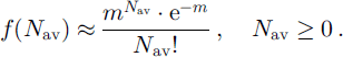
Correspondingly, the number of avalanches, Nav, occurring during any time period, At, is approximately Poisson-distributed with mean m = Δt/Δt,:
The general problem considered is that pf (and correspondingly, Δir) is not known and must be estimated. Two different approaches to this estimation problem are treated below: the classical approach, where Pf is considered a constant and the observation r is the only stochastic variable, and the Bayesian approach, where pf and r are both stochastic.
The classical approach
Within a classical statistical framework pf
is considered a constant, and the term probability has a strict frequentistic interpretation. This is equivalent to saying that
![]() In practice, n is limited, and the maximum likelihood estimator p*. = r/n is an estimator for pf
which becomes better with increasing r. If, for example, r = 1, i.e. one avalanche has occurred during an observation period of n = 200 years, the estimate p*f = 1/200 is quite uncertain.
In practice, n is limited, and the maximum likelihood estimator p*. = r/n is an estimator for pf
which becomes better with increasing r. If, for example, r = 1, i.e. one avalanche has occurred during an observation period of n = 200 years, the estimate p*f = 1/200 is quite uncertain.
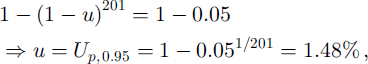
Assume now that r = 0 and n = 200, i.e. no avalanches occurred in an interval of 200 years. In this case the point estimate p*f = 0/200 = 0 is useless. Try, however, to find a conservative upper value, Up095, for pf where ”95% certain” is not exceeded, based on the observation robs = 0. A classical approach to do this is to construct a 95% confidence interval, [0, Up 095], for Pf. The upper interval limit U = Up 0 95 is then found from the cumulative binomial distribution function as follows:
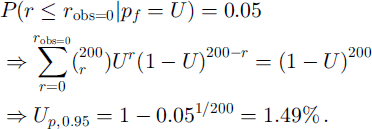
It can then be stated with ”95% certainty” that pf is not larger than 1.49% (more strictly, the observed result or less conservative results (smaller r when robs > 0) would have occurred at most 1 in 20 (5%) times if pf was really larger or equal to Up 0 95). This concept can be extended to a general certainty level, 100(1 –ε) %, and a general value for n and robs by replacing 200 with n, rohs with any value between 0 and n, 0.05 with ε, and 0.95 with 1 – ε. In this general case, however, Up i–ε is not given as a simple explicit expression and must be found numerically, based on the cumulative Bino(n, p) distribution with p as the unknown.
The advantage of the classical approach is that values for pf with specific “certainty” levels, where the term certainty and probability are defined in a strict, scientific manner, can be constructed. The disadvantage is the quite rigid concept of “an imagined infinite number of observation periods under identical conditions” needed to justify our assumptions when only a few observations are available. Another disadvantage is that when considering a specific path with only a few or no observed avalanches, it is difficult to take a priori knowledge into account (e.g. observations from other and similar paths). Here the Bayesian approach serves as a formal alternative where, for example, expert judgement can more easily be taken into account.
The Bayesian approach
Contrary to the classical approach, the parameter pf is treated as a stochastic variable with an a priori probability density function, π(pf), called the prior. The prior can be based on subjective knowledge, historical observations or both. The term prior reflects that it is established before (new) observations are made. Once new observations are available, the so-called posterior probability density function, f(pfr), for pf conditional on r can be found. The posterior, f(pfr), is proportional to π(pf) and the likelihood f(rpf), the latter now considered as a function of pf. All estimation of pf is based on the posterior. Based on a squared error loss function (Reference BergerBerger, 1980), the Bayes-estimator, p*f, for pf, equals the mean in the posterior, f(pfr).
The Bayesian approach is particularly useful if a good a priori knowledge exists (e.g. observations from similar paths) but poor observations from the actual path (e.g. r = 0). It can also be implemented, however, if no a priori knowledge is available, by applying so-called non-informative, or “vague”, priors.
Technically, the Bayes approach is particularly convenient if the prior and the posterior belong to the same class of distributions. In our case, the beta distribution beta(a, b), with mean a/(a + b), is such a conjugate class of priors, i.e.
The class of beta distributions is quite rich, including the vague prior π0(pf) = l(a = b = 1), as well as conservative (a = 1, b < 1) and non-conservative (a < 1, b = 1) alternatives. A particular choice of a vague prior, the Jeffrey’s prior πJ, is obtained with a = b = 1/2, which is invariant with respect to transformations of pf (Carlin and Louis, 1996). If, for example, p’ = ln(Pf) is considered, the probability density function of p’ will be identical to πJ if Tr(pf) = πJ. Note that πJ returns considerably less conservative estimates of pf than π0, despite the fact that they are both constructed to be vague. For large values of n, the difference between the conservative alternative and π0 IS negligible.
The empirical Bayes approach is an iterative process where the posterior from the last observation is used as a prior before a new observation. As an illustrative example, let the prior π(pf) = 1 be applied before the first year of observations, which will give one or zero avalanches. The posterior, fn(pfr), after n years of observations with totally r avalanches observed, is then
with Bayes estimate
As an example, r = 0 and n = 200 gives the estimator p*f = 1/202. Some examples of the updating procedure are shown in Figure 4.

Fig. 4. Probability distribution for annual avalanche occurrence after 0,1, 3 and 8 years of observation of no avalanche.
Analogous to classical confidence intervals, a 100(1 –ε) % credibility interval for pf, [0, Up i-£], can be constructed. In this case Up 1–ε is identical to the upper ε fractile in the posterior, which formally is found by solving the equation
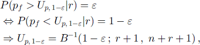
where B–1 denotes the inverse cumulative beta distribution with argument 1 – ε and parameters a = r + 1 and b = n + r+l.
Contrary to the classical approach, it is now meaningful to say that the probability of the true pf value being located in the actual interval is 100(1 –ε) %, but the probability term now does not have a frequentative interpretation due to the vague subjective probability concept involved in the prior.
If again the case r = 0, n = 200 and ε = 0.05 is considered, the cumulative posterior is
Based on Equation (17) it is therefore found that
which is very close to the value found by the classical approach. In Figure 5 the two approaches are shown for different values of ε and r. The correspondence between the two approaches decreases with increasing r, with the Bayesian approach giving the least conservative alternative. By applying Jeffrey’s prior, even less conservative estimates would have been obtained. In the Jeffrey case Up095 = 0.95%, i.e. considerably less than the estimate of 1.48% based on the flat prior. This illustrates that one should generally be careful in applying a Bayesian approach, and in particular assess the sensitivity of the choice of the prior.

Fig. 5. Comparison between classical (solid lines) and Bayesian (dashed lines) approach concerning the certainty level 1 – ε of Pf estimates for increasing number of avalanches from left (r=0) to right (r = 5) when the observation period is n 200years.
4. Applications in Hazard Zoning
4.1. Introductory remarks
As an example application, a “safe” run-out angle, αs, is now calculated based on the criterion that the annual probability of being hit by an avalanche does not exceed Ps = 1/Δts, where Δts is the “safe” period. As an example, Δts = 1000 years and Ps = 1/1000 if a ” 1000 year” avalanche is the safety criterion. A major problem is the generally poor knowledge of the return period, Δtr, or correspondingly, the annual probability of avalanche release, Pf = 1/Δtr. The certainty level assigned to the as value is therefore strongly related to the certainty level selected for the Pf estimate. The classical approach of a confidence interval described in section 3.2 is still applied, which gave results similar to or more conservative than the Bayesian approach with a flat prior. Example calculations for a Bayesian approach are presented by Reference NadimNadim (1999) and adapted to this paper by Reference Harbitz, Harbitz and NadimHarbitz and others (2001).
Further, the extreme-value model and the single-value model are considered in two fundamentally different ways to interpret the α/β model. It will be outlined how as is calculated based on each of these approaches, and a comparison will be made between them.
An important parameter involved in both approaches is ms = Δts/Δtr, i.e. the ratio between the safe period and the return period. Furthermore, the return period can be presented as a product Δtr = ΔtΔAN, where AtA is the average return period between weather situations with acute avalanche danger and N A is the average number of such acute situations between each avalanche realization.
4.2. Application of the extreme-value model
It is now assumed that the reported a angle in each avalanche path is the most extreme after N avalanches, and that N is large enough for the a angle to follow a known extreme value distribution (Gumbel). It is further assumed that both N and the observation (return) period do not vary substantially between the paths on which the α/β regression line is based. Exceptions from these assumptions may explain “outliers” in the regression analysis.
Under the assumptions above, the α/(β model is
where W is Gumbel-distributed with zero mean and standard deviation a = 2.3°. Based on the properties of the Gumbel distribution, the dynamics of the regression line is now reflected through the parameter b(ms):
As an example, assume Δtr = 200 years and Δts = 1000 years, i.e. ms = 1000/200 = 5. In this case b(ms) = –2.9°, and a(5)–0.96/3–4.3° is a possible estimate for a”safe area”. This estimate corresponds to the mean 1000 year avalanche, i.e. the mean of a huge number of imagined most extreme avalanches during many 1000 year periods. Other candidates are the modal value, analogous to how the ”100 year sea wave” is defined, and the median. Due to the skew property of the Gumbel distribution, the mean value is the most conservative choice, and the modal value is the least conservative.
Let Δas(ms) denote how much as is below the original α/β regression line 0.96/3–1.4°. The three mentioned alternatives then provide
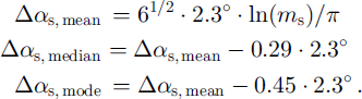
The mean is about 1 ° more conservative than the mode. The three Δas functions are shown as a function of ms in Figure 6.

Fig. 6. Distance of “safe” run-out angle, a,, from original α/β line as a function of ms based on the single-value model and the extreme-value model. Note the close relationship between extreme-value model based on mode and the single-value model.
Note that the three expressions and the differences between them strongly rely on the assumption that a is the standard deviation in the Gumbel distribution. If there are substantial differences in the number of avalanches behind the different a observations, but the Gumbel approach is still appropriate, the estimated a value also includes the N variation among paths. In this case the standard deviation in the Gumbel distribution is smaller than a, and the expressions above are too conservative.
4.3 Application of the single-value model
The α/β regression line is now
where W ∼ N(0,2.3°). As explained in section 1, the “safe-value, aαs, is now found by use of the product of run-out exceedance probability times the annual probability of avalanche release, i.e.
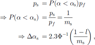
based on the properties of the normal distribution. Δαs as a function of ms is shown in Figure 6. As shown, it is very close to the corresponding extreme-value expression based on the mode in the Gumbel distribution.
If now the situation is the opposite (i.e. as = 20.3° represents a prescribed point of interest, e.g. a house or a road), the unknown ps can be found as follows: Consider an avalanche path profile with β = 25°. The prescribed point of interest along the path will be hit if a < 20.3°. From Equation (1), the expected value of a is 22.6°. The probability that an extreme avalanche will reach the prescribed point is then ps = P.
4.4. Confidence intervals for hazard zones
It has been shown how a “safe” value as can be calculated when ms is known. An assigned specified certainty level to as can be found by constructing confidence intervals [0, U/ms] for ms based on a corresponding interval [0, Up] for pf as described in section 3.2. This is due to the monotonic relationship ms = Δts/Δtr = ΔtsPf. When Up is found, Um is simply found by the relation Um = ΔtsUp. This is illustrated with the example that r = 0, i.e. no avalanches are observed during an n = 200 years period. In section 3.2 it was found that U/po95= 1–49%. With Δts = 1000 years, Um095 = 1000 × 0.0149 = 14.9. Using this value in the various Δas expressions (Equations (22) and (24)) gives:
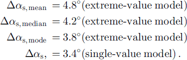
Thus, all values above are assigned a ”95% certainty level”, which could be changed to any other level 100(1 – ε) % by replacing 0.95 with 1-e.
Technically the procedure above can also be performed based on subjective judgements for a path with no avalanche observations. If, for example, avalanche experts are confident that the path is similar to other paths for which observations r and n exist, the latter can be used to estimate ΔtT, and correspondingly ms = Δts/Δtr. In this case a reasonable approach is to apply the binomial distribution with parameters Σr and Σn, i.e. the accumulated values from the similar paths.
5. Conclusion
A mechanical probabilistic model for avalanche release is applied in combination with a statistical/topographical model for avalanche run-out distance to obtain the unconditional probability of extreme run-out distance.
For the mechanical model, FORM and Monte Carlo simulations for calculating the annual probability of avalanche release are compared. The simulations give a strong indication that the FORM approximation is reasonable. The example application demonstrates that FORM is a powerful tool for performing systematic parametric studies. It provides a rational framework for decision-making when there is a large uncertainty in the input parameters, and it identifies the relative contribution of the input variables to the overall uncertainty. This information helps the engineer to focus on reducing the uncertainty in a few important parameters in order to achieve a significant reduction in the overall uncertainty.
The interpretation of the statistical/topographical model as an extreme-value model or as a single-value model is discussed. The ambiguous interpretation of the model reflects the need for more than one observation in a sufficient number of paths. It is outlined how a “safe” run-out angle is calculated based on each of the two approaches, and how a specified certainty level can be found by constructing confidence intervals based on the annual probability of avalanche release.
Comparisons of a classical approach where the probability of an avalanche occurring is a strict frequentistic constant, and a Bayesian approach with stochastic probability and a vague prior reveal that the correspondence between the two approaches decreases with an increasing number of observations, the Bayesian approach being the less conservative.
Finally, example applications in hazard zoning are presented, with emphasis on how the influence of historical observations, local climate, etc., on run-out distance can be quantified in statistical terms and how a specified certainty level can be found by constructing confidence intervals for, for example, the most likely largest run-out distance during various time intervals. Owing to the quantified uncertainty in the probability of extreme run-out distance, it is suggested that the areas susceptible to avalanches be indicated by zones rather than demarcation lines only.
It is recommended that further work on probabilistic analysis in snow-avalanche hazard zoning should:
-
1. implement probabilistic stability analysis for models that account for the way snow shear strength depends on the rate of deformation, as well as for progressive shear failure due to local stress concentration and fracture propagation on the weakness plane (unzipping mode of failure);
-
2. provide several avalanche observations in each path in order to obtain a proper interpretation of the α/3 model and the residual distribution involved, thus providing a more reliable hazard zoning;
-
3. establish uncertainty measures for the “safe” run-out angle by constructing confidence intervals for this parameter with different confidence levels, where all statistical uncertainties are taken into account, including the uncertainty of the regression line itself;
-
4. validate the α/3 model statistically and examine the sensitivity on the “safe” run-out angle measures for different choices of residual distributions.
Acknowledgements
The research project “SIP6 20001018.820 - Risk analysis” is funded by the Research Council of Norway. This support is gratefully acknowledged. F. Sandersen, K. Kristensen and K. Lied of the Norwegian Geotechnical Institute provided helpful comments. F. Rapin and M. M. Magnusson are thanked for constructive manuscript reviews.


