


Introduction
Snowdrifts can greatly influence human activities in snowy areas. Many studies of snowdrifts have been carried out over the years with experimental methods employing wind tunnels (Reference KobayashiKobayashi, 1972; Reference AnnoAnno, 1985) and water tanks (Reference IrwinIrwin, 1983). These methods usually require expensive equipment. We are developing a numerical simulation method for snowdrifts which we hope will prove useful in the design of roads and houses in snowy regions. We report here preliminary results of this recently developed method.
When wind speed exceeds a certain critical value, snow particles are entrained and are then transported down-wind. Such transport is possible either by saltation or by suspension. We have assumed that the majority of wind-driven snow particles move by saltation (Reference OhnishiKobayashi. 1972), and therefore consider only snow transport caused by this. Reference Wipperman and GrossWipperman and Gross (1985) have made several attempts to simulate the development of a sand barchan, which has a sickle-shaped form. Sand transport in barchan development is brought about mainly by saltation, so we adopt their procedure in the following three steps:
(a) Calculation of wind field, in order to obtain the friction velocity at each point.
(b) Calculation of distribution of snowdrift transport due to distribution of friction velocity given by (a).
(c) Calculation of the field of erosion and deposition rates by computing the divergence of snow drift transport.
Adding these increments to the initial height of the field leads to the new shape after a time interval. Reference Wipperman and GrossWipperman and Gross (1985) did not verify their simulation results with field data, but in our work we have been able to compare the simulated wind-velocity field and snowdrifts with those actually observed. We have adopted the finite-element method for calculation of the wind field, but it should be noted that Wipperman and Gross used the finite-difference method. Generally speaking, we can express smooth topographies easily because the finite-element method gives more reasonable answers in the case of complex boundaries than does the finite-difference method. This is very important because wind profiles near boundaries influence snowdrifts.
Figure 1 shows the model topography used. This model is constructed in wood and permits comparison of calculated results with those observed from a snowdrift outdoors. The method was developed by Reference Tabler and JairellTabler and others (1980).
Simulation of Wind-Velocity Field
The friction velocity, u*, was obtained from a velocity profile.
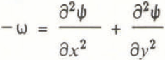
A numerical simulation method developed by Reference OhnishiOhnishi (1986) was applied in order to obtain a two-dimensional velocity field over the topography. When the viscous fluid is assumed to be incompressible, the Navier–Stokes equations in the two-dimensional case reduce to

where x and y are horizontal and vertical coordinates, u and ν are horizontal and vertical components of velocity, vt is the eddy diffusivity of momentum and ν is the kinematic coefficient of viscosity. In this paper, the eddy diffusivity of momentum was set as the constant: vt = 0.10.
By differentiating and adding together Equations (1.1) and (1.2), we get
where

Fig. 1. Schematic diagram showing an outdoor model for a snowdrift.

Fig. 2. Characteristics of topography division and air-flow conditions in calculation. Boundary conditions: at the inflow boundary, u(z) is given. At the other lateral boundary, ![]() and
and ![]() . At the upper boundary, ω = 0. No-slip conditions apply at the lower boundary.
. At the upper boundary, ω = 0. No-slip conditions apply at the lower boundary.
Since vt is generally much larger than ν, ν can be ignored. The velocities, u and v, are given by a stream function, Ψ, such that

Substitution of Equations (4.1) and (4.2) into Equation(3) gives
and Equation (2) becomes
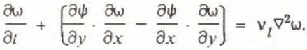
Equations (5) and (6) are those used in the simulation.
Figure 2 shows the topography on which the calculation is based and its component elements. This topography is simpler than that actually observed, in that there are no steps on the slopes and no anti-glare screen at the centre of the trench. The wind profile at the inflow boundary velocity is given by the observed wind profile, the other boundary condition is also shown in Figure 2. The simple Euler scheme is used for time integration, the time interval, Δt, being 200–300 s. The numbers of nodes and elements are 180 and 304, respectively. The friction velocity is computed from the logarithmic wind profile
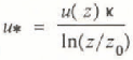
where u(z) is the wind velocity at level z; z is the height of the element nearest a surface, κ is the von Kármán constant (= 0.4), and z0 is the roughness length, taken as constant (= 3.2 × 10⁻³ cm).
This means that the wind profile is independent of saltation.
Computation of Snow Transport
The snowdrift-transport rate, q (more correctly called the vertically integrated snowdrift flux) is
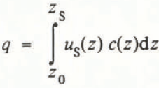
where us is the mean horizontal particle velocity, c(z) is the snowdrift density, and zs is the height of the saltation layer. Many empirical formulae have been developed for the snowdrift transport, q, in the two-dimensional case. Iversen (1980) expressed snowdrift-transport rate as a function of frictional velocity
where ρ is the fluid density, g is the acceleration due to gravity, uf is the snow-particle terminal-fall velocity, and u*t is the threshold value of frictional velocity.
The distribution of snowdrift-transport rate, q(x), at any particular point in time, is computed by applying Equation (9) using the distribution of friction velocity, u*(x).
The constant, c, was obtained by reference to the experimental data (c = 2.1, u* = 0.15 m s−1). This value is similar to that used by Reference SchmidtSchmidt (1982).
Computation of Deposition Rates
In the calculation, snow deposition was assumed to be due to a difference in the snowdrift-transport rate shown by
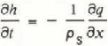
where ρs is the bulk density of snow.
The height increment, ![]() , is added to the height field h(x,i) in order to obtain a new topography, at a time-step interval Δth later, giving the relationship
, is added to the height field h(x,i) in order to obtain a new topography, at a time-step interval Δth later, giving the relationship
Reference Ishimoto, Takeuchi, Hukuzawa and NoharaIshimoto (1981) showed that the slopes for which this relationship applies could not exceed ∝0 = 30°; special treatment is therefore necessary when a slope exceeds ∝0 = 30°. The following is such a special treatment:
If ∝0 > 30° at the grid point under consideration, the topography is smoothed, and
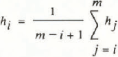
where m is the grid number at the foot of the slope.
Results
Air flow
The simulation was continued until a quasi-steady state was reached. The air-flow patterns computed and observed by using a tuft method are shown in Figure 3a and b, respectively, they are similar to each other and an especially close match is observed for separation. Figure 4a and b show respectively the contours of the computed and observed velocities. The contours are generally similar, but there are a few differences; for example, the computed velocity is a little smaller than that observed on the windward slope and in the section.

Fig. 3. Comparison of wind-direction fields; (a) calculated, (b) observed by the tuft method, in which 20 short strings were connected with a vertical bar at intervals of 100 mm.
Development of a snowdrift
The time sequences of computed and observed snowdrifts are shown in Figure 5a and b, respectively. Although their overall characteristics are similar, there was no peak in the centre of the section derived from the calculation corresponding to the presence of an anti-glare screen in the observation site. There were also differences in the total volume of drifted snow. It is suggested that these were caused by wind fluctuations which were not considered in the calculation.
It is clear that at the observation site a great deal of snow transport occurred well down the slope, and out into the base of the trench section. However, the calculation did not predict this, probably because this was due mainly to the gust problem mentioned above. In our calculations, we used mean wind speed for the observation period, which fluctuated between 6 and 8 m/s for 10 min intervals of mean wind-speed measurements. Reference AndersonAnderson (1988) reported from his calculations for sand that for decay of deposition rate the length scale increases approximately ten times when the shear velocity increases from 0.3 to 0.6 m/s. In further simulations, it is planned that wind gust should be taken into account.
Concluding Remarks
A method of simulation for the prediction of snowdrifts has been given. The results of the simulation are in reasonable agreement with those observed in a small outdoor model both for snowdrifts and for wind-velocity fields. However, it is clear that more detailed research will be necessary in order to resolve several apparent anomalies in the present work. The method is now being improved by our group in order that it should become a useful technique in the planning of roads, houses, and similar structures.

Fig. 4. Comparison of calculated (a), and observed (b), wind-velocity fields. Wind-velocity fields were observed with a hot-wire anemometer and are expressed as a ratio of wind velocity to inflow at a height of 1 m. Contours of wind-velocity ratios are shown at intervals of 0.2, and screened areas show regions with ratios greater than 0.4. In (b), dots show the positions of observation points. Wind velocity was not observed simultaneously at every point.
Acknowledgement
We thank Dr Ν. Maeno and Dr R.S. Anderson for critically reviewing the manuscript of this paper.

Fig. 5. Comparison of the calculated (a), and observed (b) snowdrifts. Shaded areas are snowdrifts


