


Introduction
Snow is an integral component of many countries’, including Norway’s, hydrologic, ecological and atmospheric system. In Norway ∼30% of annual precipitation falls as snow. An even larger part, 50–60% of annual precipitation, falls as snow in the mountainous areas in Norway and 30% of the annual runoff is from snowmelt (Reference Beldring, Engen-Skaugen, Førland and RoaldBeldring and others, 2008). Knowledge of the spatial distribution of snow is important for the prediction of water availability, forecasting snowmelt rates and runoff, assessing avalanche hazards, hydropower production planning and water resource management.
The importance of spatial snow properties in distributed snow/hydrological modeling has been demonstrated by several authors (Reference Luce, Tarboton and CooleyLuce and others, 1999; Reference ListonListon, 2004; Reference Skaugen, Astrup, Roald and FørlandSkaugen and others, 2004; Reference Skaugen Tand RandenSkaugen and Randen, 2013). Models of this type, however, require a large number of both spatially and temporally distributed data for parameter estimation, calibration and validation. One of the key problems impeding the operational adoption of distributed snowmelt models is the difficulty of retrieving datasets suitable for these purposes. This is especially problematic in areas where wind is a dominant influence on snow distribution, as in mountains, tundra and shrub lands (Reference Elder, Dozier and MichaelsenElder and others, 1991; Reference Sturm, Liston, Benson and HolmgrenSturm and others, 2001a,Reference Sturm, McFadden, Liston, Chapin, Racine and Holmgrenb; Reference Hiemstra, Liston and ReinersHiemstra and others, 2002; Reference Liston and SturmListon and Sturm, 2002; Reference Marchand and KillingtveitMarchand and Killingtveit, 2004; Reference Schirmer, Wirz, Clifton and LehningSchirmer and others, 2011). The interaction between snowfall and wind with terrain and vegetation leads to considerable snow redistribution and creates a highly variable pattern of snow accumulation (Reference Elder, Dozier and MichaelsenElder and others, 1991; Reference BaltsaviasBloschl, 1999; Reference Liston, Haehnel, Sturm, Hiemstra, Berezovskaya and TablerListon and others, 2007). The observed variability also changes with the scale of the observations (e.g. Reference BaltsaviasBloschl, 1999). These complex interactions make the sampling and modeling challenges of spatial snow formidable.
A project between the Norwegian Water Resources and Energy Directorate (NVE) and the Norwegian Meteorological Institute (met.no) called BREMS was designed to improve the national gridded (1 km × 1 km) model used in the production of snow maps for Norway (www. senorge.no). As a part of this project we needed better knowledge of the spatial distribution of snow in mountainous areas in order to validate the performance of the distributed snow model. Studies have shown that conventional methods of the arbitrary or subjective location of snow courses will not give accurate estimates of catchment snow depth in alpine catchments (Reference Elder, Dozier and MichaelsenElder and others, 1991; Reference Anderton, White and AlveraAnderton and others, 2004; Reference Erickson, Williams and WinstralErickson and others, 2005) and the large spatial variability in snow depth and snow water equivalent (SWE) in such areas makes it is difficult to obtain representative snow-depth data by traditional measurement techniques. To obtain sufficient information about the actual snow distribution with traditional means, extensive measurement designs with a large number of snow courses are required (e.g. Reference Elder, Cline, Liston and ArmstrongElder and others, 2009). The spatial resolution and coverage, repeatability and sub-canopy mapping capability of airborne lidar offer a powerful contribution to research-oriented and operational snow hydrology and avalanche science in mountainous regions (Reference Hopkinson, Sitar, Chasmer and TreltzHopkinson and others, 2004; Reference Deems, Fassnacht and ElderDeems and others, 2006). Differencing lidar maps from two dates allows the calculation of change in snow depth at horizontal spatial resolutions close to 1 m or better and over spatial extents compatible with basin-scale hydrologic needs (Reference Hopkinson, Sitar, Chasmer and TreltzHopkinson and others, 2004; Reference Deems, Fassnacht and ElderDeems and others, 2006; Reference ClineCline and others, 2009). Reference Hopkinson, Sitar, Chasmer and TreltzHopkinson and others (2004) focused on the use of lidar altimetry for measuring snow depth in forested areas but did not analyze spatial snow distributions. Other studies demonstrated that snow depth obtained from lidar could be used to characterize the spatial structure by fractal analysis of snow depth, the interannual consistency of snow distribution and scaling behavior in snow-depth distributions (Reference Deems, Fassnacht and ElderDeems and others, 2006, Reference Deems, Fassnacht and Elder2008; Reference Fassnacht and DeemsFassnacht and Deems, 2006; Reference Schirmer and LehningSchirmer and Lehning, 2011; Reference Schirmer, Wirz, Clifton and LehningSchirmer and others, 2011). Lidar snow-depth data have also been used to verify different modeling approaches, from the relatively simple statistical model to high-resolution dynamical models (Reference TrujilloTrujillo, 2007; Reference Trujillo, Ramírez and ElderTrujillo and others, 2009; Reference Mott, Schirmer, Bavay, Grünewald and LehningMott and others, 2010). However, all these earlier studies on snow distribution from airborne or terrestrial lidar are restricted to relatively small areas of 1–2 km2. In order to study the snow-depth distribution close to snow maximum in spring 2008 and 2009 in the mountainous area of Hardangervidda, southwestern Norway, we adopted airborne lidar altimetry due to its high resolution and cost-efficient features. The snow-depth data presented in this study represent a unique contribution with respect to areal extent (240 km2) and spatial resolution (2 m × 2 m) and we present results on the spatial variability of snow prior to melting for two consecutive years for a range of spatial scales (2–1000 m) and also on the use of these data to investigate the performance of the regional-scale seNorge snow model. To our knowledge, lidar data have not previously been used for verifying the performance of regional-scale models.
Study Area
This research was conducted on the Hardangervidda mountain plateau, which is situated in southwest Norway (Fig. 1). Hardangervidda is the largest mountain plateau in northern Europe. Most of the area is above the treeline, and a rich arctic flora and fauna is found. There are many lakes, streams and rivers, and much of the plateau is covered by boulder, sand, gravel, bogs, coarse grasses, mosses and lichens. The low alpine regions in the northeast and southwest are dominated by grass heaths and dwarf shrub. In the highest part in the west and southwest there is mostly bare rock or lichen/march tundra. In the east the landscape is open and flat at about 1100 m a.s.l., while in the west and south there are mountain ranges up to 1700 m a.s.l. In the far northwest the terrain plunges abruptly down to the fjord Sørfjorden.

Fig. 1. Map of Hardangervidda showing location of flight-lines.
The climate of Hardangervidda is characterized by large variations in precipitation, mostly due to the complex topography of the area. Mean annual precipitation can vary between 500 and >3000 mm over a distance of a few tens of kilometers. Hardangervidda is situated in the eastern part of the western coastal mountain range of Norway. This mountain range is a significant orographic feature oriented normally to the prevailing westerly wind flow that dominates the weather in Norway. Moist air masses are lifted by the large-scale bulk of the mountain and produce an increase in precipitation with elevation on the windward slopes, as well as a decrease on the leeward side of the range and thus on the eastern part of Hardangervidda. The snow accumulation period begins in mid-September and snowfalls persist throughout the winter months. Maximum snow accumulation is usually in mid- to late April.
Methodology
Lidar data collection
Airborne lidar data were collected for a 240 km2 area on Hardangervidda mountain plateau at a nominal 1.5 m × 1.5 m ground-point spacing. Data were collected using a Leica ALS50-II instrument with a 1064nm wavelength scanning lidar mounted in a fixed-wing aircraft with a flying height above the ground of ∼1800m. The first and last returns with intensity per pulse were recorded. Data were collected during 3–21 April 2008 and 21–24 April 2009. These dates represent the approximate time of maximum snow accumulation. A third dataset was collected on 21 September 2008. This latter dataset represents the minimum snow cover where only perennial snowpatches still exist and with leaf-off conditions. Each time a total of six flight-lines of lidar data were collected to determine the overall snow condition on Hardangervidda (Fig. 1). Each flight-line is 80 km long, follows a west-east orientation and has a scanning width of ∼1000 m. In order to reduce slope-induced errors, only a 500 m wide central part of the swath width was used. Each flight-line is separated by 10 km in the north/south direction in order to investigate any change from north to south. In addition, the lidar contractor added one flight-line that was perpendicular to the main direction in order to adjust the lines against each other. The lidar contractor, Terratec AS, collected and post-processed all data. Automated post-processing of the lidar returns, using waveform analysis and spatial filters, was used. All the Airborne Laser Scanning (ALS) datasets were delivered in Universal Tranverse Mercator (UTM) coordinates with orthometric heights. The delivered products included lidar returns classified as ground (in order to remove vegetation and buildings from the terrain), not classified and intensity. The dataset of lidar returns for Hardangervidda contained over 400 × 106 points for each survey time.
Surface DEM generation
The September 2008 mission provides bare earth ground surface elevations (although some small perennial snow-patches still exist). The April 2008 and 2009 missions provide snow surface elevation for snow-covered areas or bare ground. A 2 m resolution digital elevation model (DEM) was produced using a gridding scheme in which each original data point classified as ground was assigned to the nearest 2 m gridcell and was assumed to represent the height for the entire cell. If a subsequent data point was located in the same cell, we used the mean height to represent the height of the entire cell. The number of original data points per gridcell varied from 0 (in steep slopes and on water bodies) to 9, with a modal value of 2–3. The lidar data were collected along straight flight-lines which means that the flight plans were not designed to avoid water bodies. Therefore some of the September 2008 lidar data were measured on top of lakes or rivers of which there are many on Hardangervidda. Owing to missing data over water bodies and the possible influence of changes in water stages from water bodies, all lidar data from water bodies (as defined from maps) were removed. These areas and areas with zero original data points create large or small voids in the DEM that were not filled. A horizontal and vertical co-registration between DEMs was performed to avoid having erroneous snow-depth changes from systematic shifts between DEMs.
Following the rasterization of the lidar data, the September 2008 DEM was subtracted from the snow surface elevation (spring DEM) to produce a grid of snow depth. For each flight-line ∼8x10⁶ snow-depth measurements were obtained. The derived snow-depth point datasets (i.e. the histogram of the snow depth) along transect 2 for spring 2008 showed a distribution with long tails for both large negative (–18m) and positive (32 m) values. A similar histogram of snow depth was also found along the other transects. The negative values are obviously erroneous since they imply that the snow-covered spring surface is below the autumn surface. Some negative depths are to be expected because of measurement errors, but large negative values (defined as <–1 m) and large positive values (defined as >10m) also appear. A visual inspection of the location of the large negative or positive values indicates that most of these points occur in steep slopes or along the border of voids in the DEMs. Some of the large positive values were also associated with sharp ridges where large cornices have developed. When the overhanging mass of snow deposited falls off, a drop in elevation will occur. In steep slopes the accuracy can decrease due to horizontal errors and their effect on the vertical error (Reference BaltsaviasBaltsavias, 1999; Reference Hodgson and BresnahanHodgson and Bresnahan, 2004). A more detailed description of this error and its effect is given by Reference BaltsaviasBaltsavias (1999) and Reference Hodgson and BresnahanHodgson and Bresnahan (2004). Usually, extra overlapping flight-lines or flight-lines with different flight orientations are added in order to increase laser-shot density in areas with complex terrain and thereby improve the performance of the filtering algorithm to estimate the ground surface location. In our case, however, only one flight-line with no overlap was conducted for each transect. The present errors may thus be the result of a filtering algorithm error by the lidar contractor or from a small horizontal offset between the DEMs. Based on this consideration we have chosen arbitrarily to remove all data with negative (snow depth <–1 m) or large positive (snow depth >10m) values. The latter corresponds to somewhat larger values than the largest (8 m) observed during manual observations on Hardangervidda. For example, for flight-line 2 there was a total of 3400 points (n=8170000) with snow depth >10 m and 639 points with snow depth <–1 m. In practice, the data points removed represent <0.01% of the total area sampled and had a negligible influence on the snow-depth statistics.
As the method used to estimate snow depth relies on two measured parameters, the spring and autumn surface, the accuracy of the estimated snow depth will depend on the possible measurement errors from both. Based on the vertical error (standard deviation) of ±11 cm in surface elevation from the laser ALS50-II over well-defined surface (as stated by the manufacturer), for the sum of two surfaces one can assume an error of
![]() in the derived surface elevation change, as long as the errors in the spring and autumn surfaces are independent of each other. If we further assume that errors are normally distributed with a mean of 0 and a standard deviation of 0.15, then the negative values are set equal to 0 and an equal number of positive values (18 000) drawn from the normal distribution are also set equal to zero.
in the derived surface elevation change, as long as the errors in the spring and autumn surfaces are independent of each other. If we further assume that errors are normally distributed with a mean of 0 and a standard deviation of 0.15, then the negative values are set equal to 0 and an equal number of positive values (18 000) drawn from the normal distribution are also set equal to zero.
Lidar data validation
Absolute errors
On 15 and 16 April 2008, a kinematic ground GPS survey was undertaken along parts of flight-lines 1 and 2 for the purpose of validating the airborne lidar data. These data have been used to quantify the level of vertical error in the spring 2008 lidar data. The ground validation points were surveyed by a stop-and-go kinematic survey similar to that described by Reference Eiken, Hagen and MelvoldEiken and others (1997) using dual-frequency GPS receivers. The processed GPS data were compared with elevation obtained from the lidar-generated digital terrain model (DTM). Observed error was always computed by subtracting the in situ values from the lidar-derived values computed as: elevation error = elevation from lidar - elevation from GPS.
Relative errors (between the DTMs)
In the absence of terrestrial control points, Reference Scheidl, Rickenmann and ChiariScheidl and others (2008) proposed the use of well-defined pseudo control points (such as house edges, roof ridges, road crossings, etc.) in order to determine the relative location and elevation error between two lidar surveys. The pseudo control points must be located in areas with no expected changes between two lidar surveys. In this study well-defined pseudo control points were absent and we used differences between the spring and autumn lidar DTMs over unchanged surface (snow-free areas in the spring DTM). Hence these differences represent the relative error between elevation datasets. In order to locate snow-free areas from the spring lidar datasets the lidar intensity values were used. A qualitative visual assessment was undertaken, identifying areas with low intensity not related to steep slopes or to water bodies, in order to determine snow-free areas from the lidar intensity images (see Fig. 3a). Snow-free areas were marked manually and the elevation difference between the spring and autumn surface was computed. Ideally, these unchanged areas should be chosen randomly within the entire range of the considered surface model, but this was not possible as most of the snow-free areas are situated on convex surfaces and hilltops.
Aggregating snow-depth data
New datasets for 10, 50, 100, 250 and 500 m2 and 1 km2 resolution were generated by spatially averaging all the data points (from the original 2 m × 2 m grid) within the new resolution. The averaging was only carried out for cells where a minimum of 20% of the area was covered with 2 m × 2 m cells with measurements (e.g. for generation of a 10m × 10m DEM from a 2 m × 2 m DEM at least five 2 m × 2 m cells should be used in the averaging process). If this was not the case, averaging was not carried out and the cell was assigned a missing value. This strategy allowed us to use as many observations as possible over as large an extent as possible while trying to maintain sufficient sampling density to ensure unbiased mean value estimates.
seNorge
In Norway, daily maps of interpolated fields of temperature and precipitation with 1 km × 1 km grid spacing have been used to derive quantities like snow depth, SWE, fresh snow, etc. with the seNorge snow model (Reference Engeset and JärvetEngeset and others, 2004a). These maps are published at www.senorge.no for mainland Norway and date back to 1957. The seNorge snow model is rather simple and based on a degree-day melt model and a precipitation model both similar to those applied in the Swedish rainfall-runoff model HBV (Reference SælthunSælthun, 1996; Reference Engeset and JärvetEngeset and others, 2004a). A description of the snow model can be found in Reference Engeset and JärvetEngeset and others (2004a) and Reference SalorantaSaloranta (2012).
Results and Discussion
Elevation error
A summary of the correspondence between the spring 2008 DTM and GPS collected along flight-line 2 shows that the elevation error ranged from –0.95 m to +0.51 cm with a mean error of 0.012 m. The standard error was 0.12 m, very close to the error of 0.11 m stated by the manufacturer. As expected, a slight increase in elevation error was found as the surface slope increases. For surfaces with slopes in the range 0–48 the elevation differences ranged between ±0.2 m areas and no bias was found. These results demonstrate that there was no systematic elevation bias in the spring 2008 lidar data. A similar comparison could not be carried out for the autumn 2008 and spring 2009 data. However, there is no reason to suspect that the level of accuracy would be significantly different between the surveys since the same instrument and control parameters were used during all three surveys.
Relative elevation error
We used the statistical co-registration method described in Reference KääbKääb (2005) and Reference Nuth and KääbNuth and Kääb (2011) to investigate the relative errors between elevation data. We applied this method to stable (snow-free areas) parts of the lidar DTM. To check whether there was a systematic shift, b, or vertical offset, ä, between spring and autumn DTMs, the differences in the raster elevation were divided by the tangent of the local slope and plotted against the local aspect, ψ, according to Reference Nuth and KääbNuth and Kääb (2011):

Based on the scattered data it is possible to fit a cosine function by least-squares curve fit to estimate the parameters a, b and c (the mean vertical bias and equal to
![]() The first solution may not be the optimal solution, so iteration of the process is required (Reference Nuth and KääbNuth and Kääb, 2011). Based on data from flight-line 2, no bias was found and therefore no correction was applied.
The first solution may not be the optimal solution, so iteration of the process is required (Reference Nuth and KääbNuth and Kääb, 2011). Based on data from flight-line 2, no bias was found and therefore no correction was applied.
Snow depth variability
Figure 2 shows the histograms for the derived snow-depth points along transect 2 after removing large negative and positive values as described above. Sampled snow depths range from 0.0 to 10.0m with a mean of 2.24 m and a median value of 1.76 m. The variability is large with a standard deviation of 1.67 (Table 1). The deep snow environment along this transect produces a positively skewed distribution with a peak at zero and a long tail towards large snow depth. Similar results were also obtained from the other five transects (Table 1). This result is consistent with observations from previous studies (e.g. Reference Shook and GrayShook and Gray, 1996; Reference Marchand and KillingtveitMarchand and Killingtveit, 2005; Reference ClarkClark and others, 2011). Figure 3 illustrates the spatial variability of snow depth along a ∼500 m wide and 4000 m long transect. The section is obtained from the western part of flight-line 2 for 2008 and 2009. As can be seen from Figure 3, the snow cover exhibits a high degree of variability in space, which is apparent at a range of scales.
Fig. 2. Observed frequency distribution of snow depth along flight-line 2. Negative depths and depths >10m have been removed.
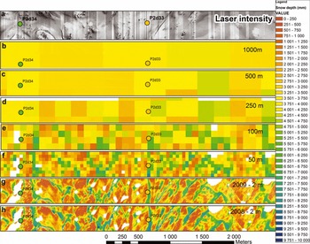
Fig. 3. Detailed spatial snow-depth distribution (2 m2) close to maximum in 2008 (h) and 2009 (g). Coarsened datasets for 50, 100, 250 and 500 m2 and 1 km2 resolution are also shown (b-f) for 2008. Intensity image (2 m × 2 m) of the same area is shown in (a).
Table 1. Statistical summary of observed snow depth (m) for 2008 for each flight-line. Mean, standard deviation, CV and skewness (Sk.) are computed for the whole dataset. Mean, minimum and maximum elevation (m) along flight-lines are also shown
At a local scale (Fig. 3g and h) snow-depth distribution in this area is characterized by a large spatial variability and qualitatively it appears to be correlated to the highly variable topography. Most of the deeper snowdrifts are situated on easterly and northeasterly slopes, in small depressions and along waterways. Areas without snow or with shallow snow cover are located primarily on hilltops, southwesterly-facing slopes and exposed level areas. At this fine scale, not only will wind-related snow redistribution and preferential deposition related to topography influence the variability, there are also effects dependent upon snow surface roughness features (e.g. dunes, ripples and sastrugi) and microtopographic features (e.g. rocks, small bumps and hallows), as well as sloughing of snow from steep slopes and avalanching. More discussion on the local-scale spatial distribution of snow in relation to surface topography is beyond the scope of this paper.
Computed snow depth at resolutions of 10 (not shown), 50 and 100 m still indicates a general pattern of snow depth that is affected by the heterogeneous surface topography (Fig. 3). One can still see the presence of high- and low-accumulation areas related to large drifts and wind scour. However, a large amount of the variability has been averaged out. The snow-depth distribution pattern is much simplified at scales of 250, 500 and 1000 m. The high- and low-accumulation areas seen at the smaller scales disappear and the variance decreases further. From Figures 3 and 4 one can see that much of the local variability is averaged out when the grid size approaches 500 m2 to 1 km2. The mean values are not affected by the change in scale (not shown), since a linear aggregating method has been used (e.g. Reference BlöschlBlöschl, 1999). Qualitatively, we can identify spatial variability of snow depth at three distinct spatial scales: (1) the hillslope scale (2–250 m) as observed from the 2 m × 2m grid along subsections of transects; (2) the catchment scale (250 m to 10 km) as observed along each transect; and (3) the regional scale (10–100 km) as the variability along the transect and between all the transects.
Fig. 4. Box plot of measured snow depth versus size of the averaging area for flight-line 2. The box on the far right-hand side (SD1000 m) shows modeled seNorge snow distribution data along flight-line 2. Numbers on top indicate calculated standard deviation.
The reduction of variance with increasing support (the support refers to the area represented by each sample; e.g. Reference Blöschl and SivapalanBloschl and Sivapalan, 1995) as seen in Figures 3 and 4 has been recognized in many studies in various disciplines of hydrology and snow analysis (Reference Blöschl and SivapalanBloschl and Sivapalan, 1995; Reference Beldring, Gottschalk, Seibert and TallaksenBeldring and others, 1999; Reference BaltsaviasBloschl, 1999; Reference Fassnacht and DeemsFassnacht and Deems, 2006). The spatial variability at local and hillslope scale (2–200 m) is dependent on local topography, wind and snow deposition/erosion processes in addition to the general climate (e.g. precipitation and temperature). The spatial variability of snow depth at spatial scales of ∼1 km is determined by the more general climate and orographic and leeward topography influences on precipitation (e.g. Reference ListonListon, 2004). The average 1 km data should therefore be more appropriate for catchment or regional model calibration than more local ground observations. Other resampling/aggregation methods such as random sampling should be used if the magnitude of the actual snow-depth variance is required (Reference Fassnacht and DeemsFassnacht and Deems, 2006; Reference Skøien and BlöschlSkøien and Bloschl, 2006). A key feature of the 1 km aggregated snow-depth data is that they do not suffer from the high sampling variability that is present at point observations. This allows for a matching of scales and results between modeled and measured values.
Interannual variation in snow depth
Wind direction, snowfall and resultant snow distribution patterns are often similar year to year (e.g. Reference Hiemstra, Liston and ReinersHiemstra and others, 2006), resulting in relatively steady-state environmental conditions. By comparing the snow-depth distribution presented in Figure 3g and h for 2008 and 2009 we find a strong interannual consistency between the two winters. Pearson’s correlation coefficient (r) between the two years was found to be r=0.95. The amount of snow is less in 2009 (mean 2.77 m) than in 2008 (mean 3.38 m), while the coefficient of variation (CV) was 0.66 and 0.71, respectively. Similar results were also found in other parts of the study area (not shown). Our results are in agreement with the findings of Reference Deems, Fassnacht and ElderDeems and others (2008), who reported large consistency between two winters with correlation coefficients of r=0.88 in areas with low rolling topography and r=0.92 in areas with moderate topography, and with the results of Reference Schirmer, Wirz, Clifton and LehningSchirmer and others (2011), who found a correlation coefficient of r=0.97 (more complex mountain terrain). Both areas studied by Reference Deems, Fassnacht and ElderDeems and others (2008) are partly covered with coniferous forest. The study area of Reference Schirmer, Wirz, Clifton and LehningSchirmer and others (2011) is more similar to our study area with a more complex terrain and negligible influence of vegetation. The findings of our study support the hypothesis formulated by Reference Schirmer, Wirz, Clifton and LehningSchirmer and others (2011) of increasing interannual consistency of snow-depth distribution at the end of the accumulation season with increasing complexity of terrain. Both Reference Deems, Fassnacht and ElderDeems and others (2008) and Reference Schirmer, Wirz, Clifton and LehningSchirmer and others (2011) indicate that the accumulation pattern found at the end of winter is dominated by a typical storm pattern and less by differences in wind direction, changing snow-pack properties and altered surface topography due to snow deposition.
Observed vs modeled snow depth
Figure 5 shows the 1 km average snow-depth values obtained from the lidar data for all six flight-lines together with the simulated seNorge value that overlaps with the same coordinates and same dates. At first glance there is an offset between the measured and modeled snow depth, but the offset decreases as we move southward and is virtually absent from the southernmost flight-line (flight-line 6; Table 2). Most of the meteorological observations used to interpolate/extrapolate temperature and precipitation fields in the seNorge model are located in low-elevation populated areas. In the area around Hardangervidda, fewer meteorological stations are present in the northwest. This may be the reason for the large deviation found between observed and modeled snow depth in the northern flight-lines. The overall seNorge model fit with observations was evaluated quantitatively by calculating Pearson’s correlation coefficient between simulated and observed values. For both 2008 and 2009 the overall correlation between measured and modeled values was r=0.77. Overestimation of snow depth by the seNorge model is on average 38% and 29% in 2008 and 2009, respectively. The better fit for 2009 is a result of a change in the overestimation along flight-line 1, which decreased from 92% to 34% between the two years. For the other flight-lines the changes are smaller (Table 2). The reason for the large change along flight-line 1 is unclear, but one likely candidate is that in the autumn of 2008 a temperature station was established at Sandhaug located in the central part of flight-line 2. This station has improved the interpolated seNorge temperature in this part of Hardangervidda. The modeled winter temperature prior to the establishment of this station seems to be lower, which implies more snow accumulation and less melting. Unfortunately, it is not possible to run the seNorge model for 2009 without the temperature data from Sandhaug, so we are not able to assess quantitatively the effect of introducing the Sandhaug temperature station. Previous seNorge snow model studies by Reference Engeset and A äEngeset and others (2004b), Reference StrandenStranden (2010) and Reference SalorantaSaloranta (2012) comparing point measurements, snow courses, snow pillows and catchment model simulations to seNorge simulated values of SWE and snow depth indicate an average overestimation in the range 86–100% of SWE in the mountainous areas of southern Norway. These studies also found, from point measurements, a general overestimation of density in the seNorge model by 100 kgm−3 at the end of the accumulation season. Snow depth in the seNorge model is therefore less overestimated than SWE (in seNorge snow depth is derived from SWE and snow density: snow depth = SWE/snow density) and Reference StrandenStranden (2010) and Reference SalorantaSaloranta (2012) found snow depth to be overestimated in the range of 50–54% in the mountainous areas of southern Norway. The bias found between modeled and measured snow depth in this study thus agrees with these previous seNorge studies and shows that the bias found in snow depth is somewhat less than for SWE since density is overestimated in the seNorge model. The rather high r value of 0.77 indicates, however, that the model performs rather well in simulating the observed variability in snow depth.
Table 2. Statistical summary of 1 km2 snow-depth data for 2008 and 2009. Observed and modeled values are shown. The difference between observed and modeled snow depth is shown in percentage difference

Fig. 5. Scatter plot between measured 1km2 average lidar snow depth and modeled snow depth for 2008 and 2009. Data for all flight-lines are shown. The positions of the flight-lines are given in Figure 1.
Regional snow-depth patterns
The main measurement results (at 1 km × 1 km scale) for 2008 are presented in Figure 6. This figure shows the spatial distribution of the observed snow depth and the simulated snow depth from the seNorge model. The general spatial patterns, such as higher accumulation on the western part and a decrease toward the east, are seen for all six flight-lines and in the simulated seNorge values. The overall trends are similar in both 2008 and 2009 (not shown) and are seen for both measured and modeled snow depths. There is a relatively strong correlation (rvalues of 0.74 and 0.75 for the measured snow depth in 2008 and 2009, respectively) between west-east coordinate and snow depth, suggesting that the leeward/rain-shadow effect east of the coastal mountain range controls the large-scale spatial variability in snow depth on Hardangervidda. Correlation between west-east coordinate and modeled seNorge snow depth is slightly higher, with r values of 0.90 and 0.75 for 2008 and 2009, respectively. Elevation has a low but significant correlation (rvalue of 0.39 (p<0.001) and 0.56 (p<0.001) for 2008 and 2009, respectively) to snow depth in both years.
Fig. 6. Relationship between west–east position and measured 1 km2 average and modeled snow depth for 2008 for all flight-lines.
A linear multiple regression analysis with west–east coordinate and elevation as predictors and snow depth as response was performed both for measured and modeled snow-depth values. Both variables were significant in the multiple regression analysis, and the west–east coordinate is more important than elevation. The results of this analysis show that the degree of explanation was relatively high for the measured snow depth, with r values of 0.80 and 0.86 in 2008 and 2009, respectively. The values for the modeled snow depth were 0.94 and 0.86, respectively. As this correlation indicates, the variability in snow depth on Hardangervidda at the 1 km2 scale can be well predicted by west–east coordinate and elevation. The variability is lower (CV =0.26) for the simulated seNorge values compared with the measured values (CV =0.40), suggesting that the 1 km2 average values are effected by processes not captured by the seNorge model. The seNorge model snow accumulation and snowmelt are calculated by applying a simple degree-day model and a mass-balance accounting procedure. The model neglects important physical processes associated with the subgrid-scale temporal and spatial variability of snow. The relatively coarse resolution of the snow-depth estimation in the seNorge model or in similar regional snow models cannot resolve small-scale snow-depth variability, so this variability is averaged out across the grid element (Reference BlöschlBlöschl, 1999). Hence, these models have to rely on the ability of ground-based observations to represent the average conditions of subgrid element variability (e.g. Reference Molotch and BalesMolotch and Bales, 2005). However, the relatively high correlation between the modeled and measured snow depth shows that most of the variability in snow depth is explained by the model. Also, the mean processes that determine the spatial snow-depth distribution over Hardangervidda are well described in the model. This implies that the interpolated and extrapolated temperature and precipitation fields used as input to the seNorge model capture the most important features of snow accumulation. How the spatial patterns of snow depth evolve through the melting season has not been investigated in this study.
Conclusions and Perspectives
This study used an airborne lidar dataset to investigate the spatial distribution of snow on Hardangervidda. At the local and hillslope scale we found large spatial variability for snow depth in the range of 0 up to at least 10m and the distribution of snow depth is clearly positively skewed. Mean values of snow depth over areas with increasing size have been calculated using all available observations in the given area. Results show that the spatial variability of snow depth decreases as the area of averaging increases. The variability of snow depth sampled for smaller areas is affected by local redistribution, preferential deposition processes and local topography, and may mask out the large-scale snow distribution pattern. The 1 km2 average snow-depth dataset has been used for evaluating the regional-scale seNorge snow model. Results show good agreement in spatial pattern between 1 km lidar snow depth and the seNorge modeled snow depth, with a pronounced bias in the mean snow depth. At the regional scale the west–east coordinate is a more important predictor of snow depth compared with elevation on Hardangervidda.
The work presented here indicates that 1 km2 average snow-depth data will give an adequate representation of the average grid element snow depth. With the acquisition of this dataset it is possible, in principle, to evaluate and develop snow models for many spatial scales. Furthermore, the detailed lidar data make it possible to determine spatial frequency distributions of snow at different scales that can be used to improve the runoff dynamics of spring floods (Reference Luce, Tarboton and CooleyLuce and others, 1999; Reference SkaugenSkaugen, 2007; Reference Skaugen Tand RandenSkaugen and Randen, 2013).


