


Introduction
Ice-sheet modelling is an essential tool in evaluating the future response of ice sheets to climate change. Models need as many tests as possible to enable a judgement to be made on the performance of models. Every time a model passes a test, more confidence may be placed in model results for periods without control options such as the future. They should especially be evaluated for circumstances and time-scales in which they will be used (Oreskes and others, 1994).
The large spatial and long-term temporal scale of ice-sheet models limits the amount of data which can be used to test model results. Modelled ice-sheet geometry (span, topography, volume) can be compared with present-day geometry for the Greenland and Antarctic ice sheets. Modelled ice temperature can be tested against measured temperatures at deep drilling sites in Greenland and Antarctica.
The potential of the geological record to provide test data for ice-sheet models is often mentioned (e.g. Paterson, 1981; Hindmarsh, 1993). However, systematic comparisons between geology and ice-sheet models are not widespread. Data in geology are diverse in nature (morphological, sedimentological) and occur on a wide range of scales, in size and time. Not all types of geological data can be used in comparisons with ice-sheet model results. Based on the approach of Tatenhove and others (in pressa), only those geological features are used which relate directly to model output. The geological record used here is a sequence of dated moraines. Moraines are the morphological expression of the ice-sheet margin and therefore relate directly to modelled ice-sheet geometry.
Using a geological record for testing ice-sheet models is useful because it provides test material on the time-scales typical for the memory of ice sheets (millennia). It also enables the analysis of transient behaviour of ice-sheet models.
The aims of this paper are:
-
To compare modelled positions of the ice margin of three Greenland ice-sheet models with geological evidence.
-
To evaluate the performance of the three models with respect to the geological record.
-
To discuss the differences in performance between the three models in terms of model characteristics.
Geological Record
For this paper we used the morphological evidence of ice-margin positions as provided by moraine systems. Moraine systems are clusters of moraines which are traceable over large distances (10–100 km). Regional significance is attached to these systems because they are traceable over large areas and continue without being interrupted by topographic features such as valleys (e.g. Ten Brink, 1975). The positions of moraine systems (Fig. 1) are taken from various sources (for a review see Tatenhove, 1995; Tatenhove and others, in pressa). A detailed discussion on the methodology used in constructing the geological scenario is given in Tatenhove and others (in press a).
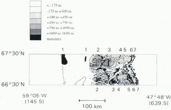
Fig. 1. Overview of moraine systems in central West Greenland. 1, Hellefisk-Sisimiut; 2, Taserqat; 3, Sarfartôq/Advedtleq; 4, Fjord; 5, Umîvît/Keglen; 6, Ørkendalen; 7, Present-day ice margin. Figures in brackets below the longitude denote the UTM coordinates (easting) in km used in Figure 3.
Table 1. Deglaciation chronology of West Greenland. Division in groups is based on the availability and type of age determination. A, no 14C dates available in offshore area; B, ages based on radiocarbon-dated marine shells; C, ages based on radiocarbon-dated terrestrial material; D, no 14C dates available in area presently covered by ice sheet

Table 2. Table 2. Model features

Moraine systems were dated by 14C-dated marine shells and terrestrial peat, and were divided into four groups depending on the way ages were determined (table 1). Groups A and D contain moraine systems without 14C-dates. The relationship between relative sea level, which holds geological remnants with 14C-datable material, i.e. marine shells and moraine systems, is used to provide ages for group B. Group C is dated by terrestrial organic material found between morainic ridges. Although some 14C dates can be used to constrain the age of group D, this group does not give direct evidence of position, because it is presently covered by the ice sheet.
The ages of moraine systems are based mainly on the work of Ten Brink and Weidick for group B (Weidick, 1972; Ten Brink and Weidick, 1974; Ten Brink, 1975). The ages of the Umîvît/Keglen, Ørkendalen systems and group D have been discussed by Tatenhove (1995) and Tatenhove and others (in press b). The age ranges of the moraine system include the time period encompassed by the moraine system, the error related to the 14C dating itself and the uncertainty due to the inconclusive relationship between 14C date and moraine system. For the Hellefisk and Sisimiut moraines, no 14C dates are available within the research area and the assigned dates are based on arguments given in Tatenhove (1995). Moraine systems with a limiting 14C date close to the former ice margin (Fjord, Umîvît/Keglen) have a relatively small age range.
Moraine-system age and associated accuracy ranges are interpolated to a 1 km × 1 km grid over an area of about 57 500 km2. Re-sampling to the area covered by a model grid point enables a quantitative comparison with modelled ice-margin positions.
Glaciological Models
The three models used in this study all cover the entirety of Greenland. An overview of the fundamental mathematical equations and model characteristics can be found in Fabre and others (1995) for the model denoted with “Fabre”, in Greve (1995) for the model “Greve” and in Huybrechts (1994) for the model indicated by “Huybrechts”. These models are based on the model discussed in Huybrechts and others (1991). The three models calculate the three-dimensional temperature and velocity field in the coupled mode to account for the temperature-dependent deformation of ice. The softness parameter of ice, which determines the rate of deformation, is a function of both temperature (all models) and the age of ice (“Huybrechts”, “Greve”). Mass flow is by internal deformation and by basal sliding in the case of temperate basal temperatures (all models).
The models use the same data set for present-day bedrock topography (Letréguilly and others, 1991). The models calculate isostatic bed adjustment with a time lag due to asthenospheric viscosity. The temperature evolution in the lithosphere is calculated up to a depth of several kilometres.
Present-day surface temperatures and accumulation rates are derived from Ohmura (1987) and Ohmura and Reeh (1991). The parameterization of surface temperature is in all three models treated as deviation from present-day values, using the ice-core record of GRIP (Fabre, Greve) or a compilation of the Dye 3 and Camp Century records for the period since the Last Glacial Maximum, after correction for elevation changes and origin of the ice (Huybrechts; Table 2) to estimate past values. No account is given for the spatial variability in time. The parameterization of accumulation is also expressed as deviation of present-day values. The Fabre model includes an orographic component, thereby creating some spatial variability in time in the accumulation pattern.
Sea-level change is ignored by the Greve model and is dealt with in a conceptual manner by the Fabre model (table 2). The Huybrechts model uses the New Guinea record (Chappel and Shackleton, 1986) to force sea level.
The grid size of the models is 20 km (“Fabre”, “Huybrechts”) and 40 km (“Greve”). The Greve model has used two different forcing functions. “Grevel” used a smoothed GRIP record (2000 year averages), while “Greve2” used the original, unsmoothed GRIP data. The position of grid cells of the three models is given in Figure 2.

Fig. 2. Position of grid cells of three Greenland ice-sheet models (Fabre, Greve and Huybrechts). The area covered is equal to Figure 1. Black cells denote the modelled position of the present-day margin.
Results
The modelled ice margins of the Greve and Huybrechts models are generally older than the margin age derived from the geological record (Fig. 3). The average differences between the models and geology are 900 and 650 years, respectively. The Fabre model produces similar differences on the present-day offshore area, but it is in close agreement with the geological record onwards (Fig. 3). For this model, the average difference with the geological record is 400 years for the present-day land area. The deglaciation rate is reasonably reproduced by all models (Fig. 3).

Fig. 3. Distance (in UTM) from west to east versus geological and modelled ages of ice-margin position (expressed in 103calendar years). The figure displays modelled ages for the x coordinates of the grid cells shown in Figure 2. It is assumed that the minimum extent of the ice sheet was 50 km behind its present position. The continuous line gives the average geological age of moraines.
As illustrated in figures 3 and 4, modelled positions of the ice margin become closer to the geological scenario after about 10 ka BP or from 445 km UTM (Universal Transverse Mercator) eastward. Before this period, the difference between geology and model is much larger (Fig. 4). The modelled deglaciation rate is similar to the geological deglaciation rate for the land area between 445 and 500 km UTM or for the time period 10–6 ka BP (Fig. 3).

Fig. 4. Modelled time of position of the ice margin versus moraine age derived from the geological record, assuming the minimum extent of the ice sheet is 50 km behind its present position. Error bars indicate the uncertainly in age of former ice-margin positions. Because this uncertainty depends on location and is sampled around model grid-point coordinates (which differ for each model), error bars at equal geological time may differ in size.
There are larger differences between the three models regarding the timing in reaching the present-day coastline. Moraines near the coast have an estimated age of 11–10 ka BP. The margin is at the present-day coastline at 18 ka BP in the Greve model (where it slays till 12 ka BP), between 14.5 and 12.5 ka BP in the Huybrechts model and between 12 and 10 ka BP in the Fabre model.
The Ørkendalen moraines are close to the present-day ice margin and have an age of 7.1–6.5 ka BP (Tatenhove and others, in press a). Grid cells at the positions of these moraines have a marginal position at 7.5 ka BP (“Huybrechts”), 8.5 ka BP (“Greve”) and 6.4 ka BP (“Fabre”). The ice sheet retreated after the Ørkendalen period behind its present position. In the Huybrechts model, this retreat comprises two grid cells (i.e. 40 km) behind the modelled present-day position. For the Greve model, this distance is one grid cell (i.e. 40 km, the Greve2 forcing). Apparent differences exist between “Greve1” and “Greve2”. While the ice-sheet margin is fixed in position after 8 ka BP in “Greve1”, the output of “Greve2” shows a more dynamic behaviour of the ice sheet after the Ørkendalen period (Fig. 4).
Discussion
How can we explain the observed differences between the models and the geology and also between the three models in terms of model characteristics? In this discussion we concentrate on the topics described above.
The contrast between the poorly modelled ice-margin positions in the coastal area and the reasonably well modelled deglaciation pattern on land may be sought in the period prior to 12–10 ka BP. The modelled ice sheet does not reach the present-day coastline in time and continued deglaciation is postponed until 11 000 calendar years BP by climate cooling related to the end of the Bølling/Allerød and Younger Dryas. In the near-coastal areas, large uncertainties exist in the geological model. Nevertheless, if we assume that the geological record is correct, we may conclude that modelled ice-margin positions for the Fabre and Huybrechts models during the period 15–12 ka BP are flawed. This is probably related to an incomplete treatment of the influence of sea level on ice-marginal ice wastage. This may occur because isostatic effects that cause a regional deviation in relative sea level in West Greenland from the global sea-level record of Chappell and Shackleton (1986) used In “Huybrechts” are not sufficiently modelled, or as a result of the internal model physics, i.e. the calving method adopted. The effect of sea-level forcing can be illustrated by the time at which modelled ice sheets reach the present-day coastline. Greve’s model ignores sea-level change and has a difference of 8 ka with the geological record. Using present-day sea level does not allow the ice sheet to expand on the present-day shelf. When sea-level changes are included, the ice sheet can expand on to the shelf The deglaciation on the present-day shelf is sensitive to the prescription of sea level and ice wastage. These two factors determine whether the age of modelled margins in the coastal area is in agreement with the geological record. Considering the time at which the ice sheet reaches the present-day land area, the conceptual treatment of sea level used by “Fabre” works out well. The age difference between models and geology which develops due to the incorrect treatment of sea level on ice-marginal ice wastage has consequences for the modelled ice-margin position in the land area. This may explain the postponed retreat in the coastal area for the Huybrechts model. The Fabre model is slightly ahead of the geological record in the on-land area. The difference between Fabre and Huybrechts is probably related to differences in the ice-core records used.
The deglaciation rate is reasonably modelled by all three models. Part of this success may be attributed to the absence of ice streams in the area. Although large fjords exist, ice streams probably only developed in the near-coastal area. Ice streams are an extreme ease of ice motion determined by basal processes. The role of basal sliding in determining ice-margin positions is probably relatively unimportant in the part of the West Greenland area examined in this study. However, a basal-sliding module may be a crucial prerequisite to model relatively large fluctuations (retreat and advance) such as occurred around the Holocene climatic optimum or during the cold spell around 8.0 ka ago. In the marginal area, mass flow via basal sliding makes a rapid advance possible, with moderate ice thicknesses in marginal grid cells, relative to the case that ice thickening in the marginal grid cells must originate by ice creep only. The moderate ice thicknesses in marginal grid cells can subsequently easily ablate. Therefore, basal sliding enables the ice sheet to become more dynamic in its response to climatic forcing.
The synchrony in deglaciation rate between the models and the geology further implies that the increased ablation during deglaciation predicted by the parameterization of surface melt is reasonably correct. An important factor which determines this success is the quality of the forcing, i.e. the ice-core records used.
Alter the Ørkendalen period, the ice margin retreated behind its present position. Near Jacobshavn, Weidick and others (1991) found evidence for a substantial retreat within this period known as the hypsithermal or Holocene climatic optimum. The recession is conceived as “natures own greenhouse experiment” (Weidick and others, 1991) and provides the opportunity to judge the performance of models which are used to depict future changes of the Greenland ice sheet.
The Greve2 and Huybrechts models generate a retreat behind the present-day ice margin. Differences between Greve2 and Huybrechts are probably related to the origin of the forcing (GRIP versus Dye 3/Camp Century). The GRIP record may be less valuable for the Holocene, because it is not corrected for flow effects. The representation of the signal of the Holocene climatic optimum is also too weak in the GRIP record (paper in preparation by S. Johnson and others).
A remarkable phenomena is that model Greve1, which is fed by a smoothed version of the CRIP curve with 2000 year averages, does not produce a dynamic, fluctuating ice sheet around the Holocene climatic optimum. When the unsmoothed GRIP data are used (in Greve2) the ice sheet advances to its present-day position following a retreat of one grid point. The GRIP record, used to force surface temperature and accumulation, does not show a large climatic change throughout the Holocene (Dansgaard and others, 1993). The already weak climatic signal related to the Holocene climatic optimum is eliminated by smoothing.
An additional effect may be the impact of short-term (decadal) fluctuations in climatic variables on the position of the ice margin. Many short-term fluctuations in δ 18O can be observed in the GRIP record during the Holocene. These fluctuations have a duration of decades and a magnitude of about 0.5‰, and some have a periodic nature (Tatenhove, 1995). The impact of these fluctuations are probably not detectable within the spatial resolution of the ice-sheet models discussed, because the associated fluctuations of the ice margin have a magnitude of several hundreds of metres up to several kilometres. Experiments with a surface-energy balance model of the Greenland ice sheet showed that random variations, with a frequency of 2 years, cause an increase of ablation by 10% under constant climatic conditions (Wal and Oerlemans, 1994).
Therefore, it is suggested that the elimination of the weak climatic signal by smoothing, and possibly the effect of decadal fluctuations in ablation and accumulation rate, explain the difference between models Greve1 and Greve2. It clearly shows the sensitivity of modelled ice margins for trends in forcing with long-term or short-term signals. Models which are going to be used to evaluate the future geometry of the ice sheet should include the effect of short-term variability in climatic parameters.
Conclusions
All three models for which results are discussed belong to the same class of model, i.e. they take account of the coupling of temperature and velocity fields on a three-dimensional network. Despite this similarity, distinct differences exist in modelled positions of the ice margin in West Greenland from the Last Glacial Maximum to the present. Disagreement between the geological record and modelled margins in the near-coastal area can be explained by inadequate modelling of marginal ablation in a tide-water environment, either by inadequate forcing functions for sea-level fluctuations or by an insufficient parameterization of caking.
The parameterization of surface melt and surface temperature based on the GRIP or Dye 3/Camp Century data (Dansgaard and others, 1993; Huybrechts, 1994) is capable of simulating the pattern of deglaciation rather well. This success may partly be the result of the apparently subordinate role of basal processes (sliding, bed deformation) in the study area in West Greenland.
The Greve and Huybrechts models show a smaller ice sheet than at present during the Holocene climatic optimum. In the case of the Greve model, this smaller ice sheet only occurs when an unsmoothed forcing is used which correctly treats the climatic signal related to the Holocene climatic optimum.
During the Holocene, short-term variations in ablation as depicted by ice-core records will result in margin fluctuation of several kilometres at best. Such fluctuations are not delectable using present-day ice-sheet models. However, the length of the ice margin in West Greenland which is sensitive to fluctuations during the Holocene climatic optimum is about 600 km (Weidick, 1993). Fluctuations of the ice margin with a magnitude of several kilometres may therefore cause global sea-level changes of several tens of millimetres. This underlines the importance of a more refined spatial resolution of models and the incorporation of short-term variations in climatic variables.


