


INTRODUCTION
The floating ice shelves surrounding much of the Antarctic coastline limit mass flux from the interior of the continent (Thomas, Reference Thomas1979; Dupont and Alley, Reference Dupont and Alley2006). As a result, changes in ice shelf geometry and dynamics can cause changes in the mass of grounded ice. Ice shelf attributes such as thickness, flow and grounding line position depend in part on the budget of forces in the floating ice. The force budget, in turn, depends on resistive forces originating in lateral drag along embayment walls and areas of localised grounding on elevated seabed topography, called pinning points (Matsuoka and others, Reference Matsuoka2015).
Pinning points provide resistance to ice shelf flow by modifying the balance of forces within the floating ice. Each pinning point and the grounded ice above it forms, in effect, an obstacle to ice shelf flow. The obstacle generates a reaction force that acts upstream, in opposition to the gravitational driving stress that compels the ice to flow. Because the balance of forces in floating ice is non-local, this reaction force has an effect everywhere in the ice shelf. Of particular interest with respect to ice-sheet stability, pinning points may affect the dynamics of the grounding zone and tributary glaciers, potentially decreasing mass flux in comparison with unrestrained flow (Goldberg and others, Reference Goldberg, Holland and Schoof2009; Favier and others, Reference Favier, Gagliardini, Durand and Zwinger2012; Fried and others, Reference Fried, Hulbe and Fahnestock2014; Favier and Pattyn, Reference Favier and Pattyn2015). The magnitude and significance of the dynamic effect appears to depend on the sizes and locations of pinning points (Matsuoka and others, Reference Matsuoka2015) although this has not been examined in detail.
As localised grounding modifies the balance of forces, further mechanical effects arise. Compression upstream of a pinning point generates thickening, which itself modifies the force balance and may cause additional grounding (Fried and others, Reference Fried, Hulbe and Fahnestock2014). Shear along the margins of a pinning point resists ice shelf flow but shearing may also generate crevasses, rifts and other mechanical effects such as the development of a crystal preferred orientation (MacAyeal and others, Reference MacAyeal, Rignot and Hulbe1998; Hulbe and Fahnestock, Reference Hulbe and Fahnestock2007; Hudleston, Reference Hudleston2015). Over time, this may reduce the resistive effect of a pinning point. Downstream of a pinning point, extension together with a redirection of mass flux causes the ice to be thinner than it would otherwise be. Indeed, the non-local nature of the momentum balance in floating ice means that any local change in ice thickness must have shelf-wide consequences as explored, for example, by Campbell and others (Reference Campbell, Hulbe and Lee2018) and Reese and others (Reference Reese, Gudmundsson, Levermann and Winkelmann2018). All together, these effects may modify the spatial pattern of a pinning point's influence on the overall force budget over time.
Pinning points can be classified according to their geometry. Ice rises have a distinct dome-shaped topography associated with stagnant or very slow ice motion over a frozen base. Ice shelf flow diverges around the topographic rise and ice rises are often elongated in the direction of ice flow. Ice rumples have more irregular shapes and are relatively small compared with ice rises, rising <100 m above the ice shelf surface. The ice in a rumple is in contact with the sea floor and continues to flow directly over the grounded area. Despite their relatively small size, ice rumples still play an important role in determining the balance of forces within an ice shelf (e.g., Berger and others, Reference Berger, Favier, Drews, Derwael and Pattyn2016).
Ice rises and rumples are common features of the Ross Ice Shelf (RIS), Antarctica's largest ice shelf. Large ice rises include Crary Ice Rise (CIR), Roosevelt Island (RI) and Steershead Ice Rise (SIR) (Fig. 1). Many smaller, unnamed ice rumples are located in the eastern sector of the RIS, near the Shirase and Siple Coasts. With the exception of RI, ice rises and rumples are largely absent across the calving front and in the central and western regions of the RIS. The majority of the RIS pinning points are distributed downstream from the large, fast-flowing Siple Coast ice streams that form the main pathway for ice flowing from the interior of the West Antarctic Ice Sheet (WAIS) to the RIS.
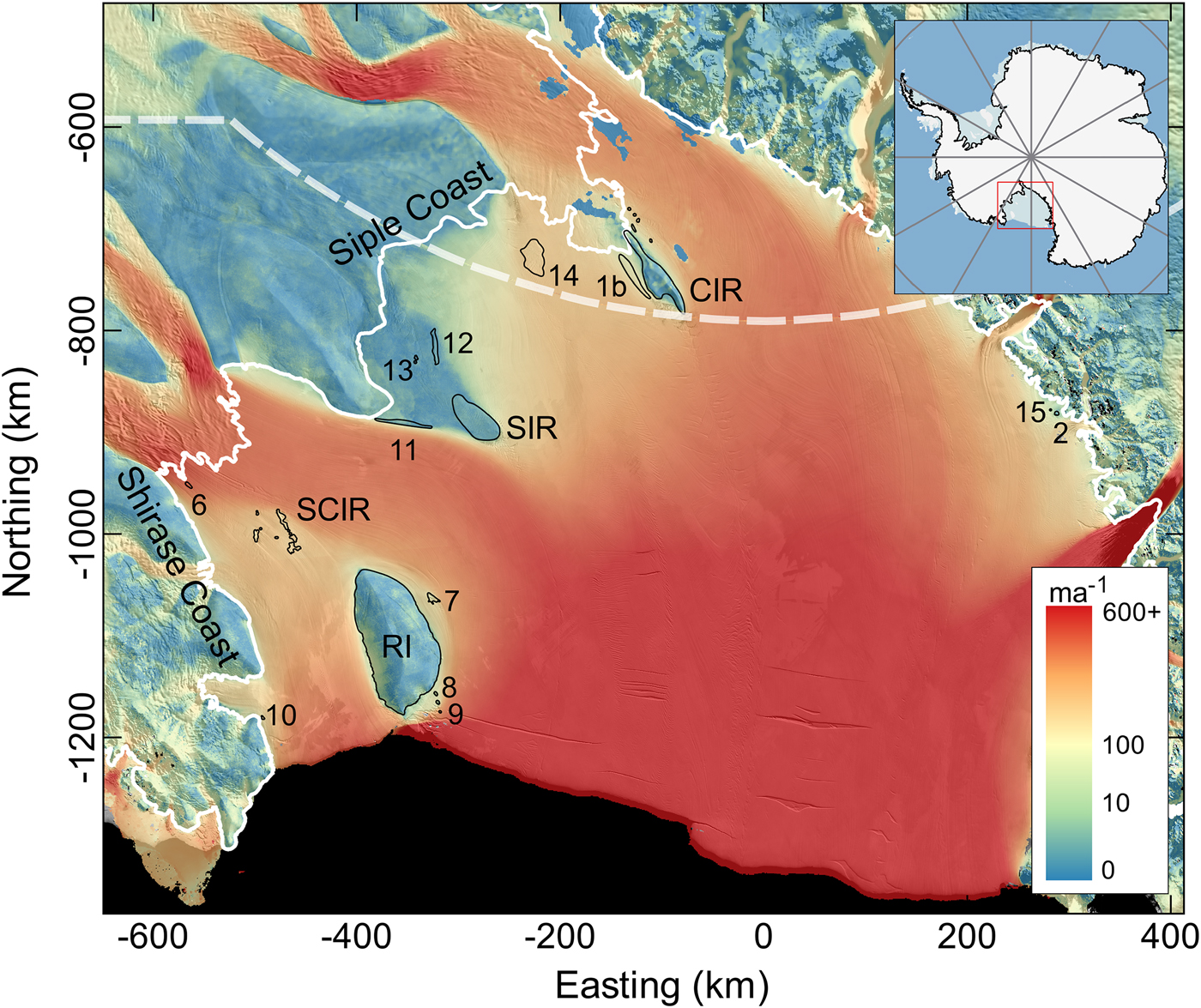
Fig. 1. Pinning points within the Ross Ice Shelf. Larger pinning points are labelled: SCIR = Shirase Coast Ice Rumples, RI = Roosevelt Island, CIR = Crary Ice Rise, SIR = Steershead Ice Rise. The colour map of velocity magnitude is a synthesis of the Landsat 8 and MEaSUREs velocity data overlayed onto the MODIS MOA (Haran and others, Reference Haran, Bohlander, Scambos, Painter and Fahnestock2014). The white line represents the grounding zone (Bindschadler and others, Reference Bindschadler2011).
Since the Last Glacial Maximum, the grounding zone of the WAIS/RIS has retreated ~1300 km inland from the continental shelf edge (Conway and others, Reference Conway, Hall, Denton, Gades and Waddington1999). Continental shelf morphology has mediated the RIS's prolonged history of retreat (Anderson and others, Reference Anderson2014; Matsuoka and others, Reference Matsuoka2015). Although the RIS is relatively stable (Pritchard and others, Reference Pritchard2012; Campbell and others, Reference Campbell, Hulbe and Lee2018), model simulations project a pattern of greater basal melt rates in the eastern sector of the RIS generated by the inflow of water masses from the east (Schodlok and others, Reference Schodlok, Menemenlis and Rignot2016). Basal melting can result in both grounding line retreat and detachment from pinning points. With this unpinning, the balance of forces across the whole ice shelf will change, and as a result, ice flow speed and thickness will change as well. Pinning points will continue to mediate the response of the RIS to climate change, albeit with different configurations than at present.
Here, we quantify the mechanical effects of pinning points in the RIS as they appear today using a force budget approach (MacAyeal and others, Reference MacAyeal, Bindschadler, Shabtaie, Stephenson and Bentley1987). This approach partitions drag exerted on the ice shelf into components arising from different processes. The magnitude of the net effective resistance we calculate using these components is analogous to Fürst and others (Reference Fürst2016) maximum buttressing number. First, we present a detailed mechanical inventory of the RIS pinning points. Second, the resistive forces exerted by the RIS pinning points on surrounding ice shelf flow are quantified. Several pinning points are examined in detail with the aim of elucidating the full range of effects that pinning points may have on ice shelf behaviour.
RIS PINNING POINTS
Fifteen pinning points and pinning point complexes are considered here. The coastlines of the associated ice rumples and rises were digitised from the MODIS Mosaic of Antarctica (MOA; Haran and others, Reference Haran, Bohlander, Scambos, Painter and Fahnestock2014) and individual Landsat 8 panchromatic band images. The resolution of the imagery is 250 and 15 m, respectively. Where ice rumple perimeters were indistinct, changes in ice surface elevation associated with localised grounding were identified in the Geoscience Laser Altimeter System (GLAS) 500 m DEM of Antarctica (DiMarzio, Reference DiMarzio2007). The traces of some ice rumple perimeters differ in detail from those inventoried by Matsuoka and others (Reference Matsuoka2015) and one additional feature, a very small ice rumple (3 km2) nearby Deverall Island (#2), is included (ice rumple #15) (Fig. 1).
The persistence of each pinning point can be inferred from downstream flow features in the ice shelf such as crevasses and streaklines (Fahnestock and others, Reference Fahnestock, Scambos, Bindschadler and Kvaran2000). Streaklines stretching downstream from CIR and the Shirase Coast Ice Rumples (SCIR) extend to the ice shelf front indicating that these pinning points are long-lived features, persisting for hundreds of years. The crevasse track originating from SIR does not extend to the ice shelf front and it can be inferred that the ice rise became well-grounded 350--400 years ago (Fahnestock and others, Reference Fahnestock, Scambos, Bindschadler and Kvaran2000). Traces downstream of the small pinning points offshore from RI are visible only a few kilometres downstream, indicating formation within the last 100--200 years although snow cover may obscure part of the record. Where they are long-lived, changes in streakline character may reveal changes in pinning point morphology and degree of grounding over time. A streakline originating from the easternmost edge of the SCIR is wider and more undulating further downstream than closer to the ice rumples, suggesting a greater degree of grounding or a larger feature between 400 and 700 years ago. Smaller rumples or lightly grounded features do not generate crevasse patterns or streaklines that are detectable in satellite images and their persistence over time is more difficult to investigate.
DATA
Velocity and strain rate
Strain rates derived from observed ice shelf flow are used in the ice mechanics analysis. Here, components of the infinitesimal strain rate tensor  $\dot {\epsilon }_{ij}$ are calculated as spatial gradients in the surface velocity field
 $${\dot \epsilon}_{ij} = \displaystyle{1 \over 2} \left[{\displaystyle{\partial u_{i}} \over{\partial x_{\,j}}} + {\displaystyle{\partial u_{\,j}} \over {\partial x_{i}}}\right]$$
where the subscripts i and j represent the horizontal directions x and y, and u represents the flow velocity with components u x and u y.
Two different velocity datasets are used in the present work. North of 82.5°S, strain rates are calculated from the Landsat 8-derived flow velocity dataset (K. Alley, pers. comm., 2016, Fahnestock and others, Reference Fahnestock2016). The resolution is 750 m and errors on individual velocities vary from 5 to 10 ma−1. This dataset represents the time interval between 2013 and 2016 when the images were acquired. South of the Landsat 8 limit, we use the MEaSUREs velocity dataset, available at 450 and 900 m resolution (Rignot and others, Reference Rignot, Mouginot and Scheuchl2011a). The 900 m resolution product, which has data gaps but lacks some of the artefacts present in the 450 m resolution product is used in the ice mechanics analysis to minimise artefacts in the strain rate calculation. This velocity product was assembled from multiple interferometric synthetic aperture radar datasets acquired between 2007 and 2009 with errors varying from 3 to 5 ma−1 over the RIS (Rignot and others, Reference Rignot, Mouginot and Scheuchl2011b). Errors on strain rates computed directly from the gridded velocity would be very large, of the order of 0.01 a−1. Thus, strain rates are averaged over several grid cells to reduce noise, as discussed further in the Application section.
Ice shelf thickness
Ice shelf thickness may be inferred from surface elevation (freeboard) by assuming that the ice is floating in hydrostatic equilibrium (e.g., Griggs and Bamber, Reference Griggs and Bamber2009; Le Brocq and others, Reference Le Brocq, Payne and Vieli2010). The thickness H is calculated
 $$H = {\displaystyle{(s-f)\rho_{\rm w}} \over {\rho_{\rm w}-\rho_{\rm i}}}+f$$
where s is the surface elevation above mean sea level, ρ w is the density of ocean water (1028 kg m−3) and ρ i is the density of ice (917 kg m−3). Where ice runs aground, the difference between the surface elevation and the Bedmap2 bed elevation is computed. The firn density correction f reduces H to the ice shelf thickness when the firn layer is compacted to ρ i. f on the RIS varies between 16 and 19 m (van den Broeke and others, Reference van den Broeke, van de Berg and van Meijgaard2008). s is obtained from the GLAS 500 m DEM of Antarctica (DiMarzio, Reference DiMarzio2007). This DEM was created from repeat observations of surface elevation acquired between February 2003 and June 2005.
Each measured value in Eqn (2) introduces error into the final ice shelf thickness map. The firn correction has a reported uncertainty of 4 m along the RIS grounding line (van den Broeke and others, Reference van den Broeke, van de Berg and van Meijgaard2008). The original authors of the GLAS 500 m DEM do not report its uncertainty, though a related analysis on the Amery Ice Shelf uses 0.08 ± 0.82 m for the mean and standard error (Wen and others, Reference Wen2010). In view of this, a conservative estimate of the uncertainty in surface elevation, 1 m, is used here, although the actual uncertainty for the RIS is probably much smaller due to its low surface slope. Uncertainties associated with each component are added in quadrature (Taylor, Reference Taylor1997, p. 75). All together, the uncertainty in H is 34.3 m (1σ). In comparison, the Bedmap2 ice thickness has a reported error of 150 m for the RIS (Fretwell and others, Reference Fretwell2013). Uncertainty in H is used later to assess the uncertainty in the force budget components.
The thickness of ice above buoyancy H ab indicates the degree of groundedness of a pinning point. When H ab is larger, tides are less likely to affect the ice and more thinning (or sea-level rise) is required to lose contact with the sea floor. For reference, the tidal amplitude in the RIS cavity is <±1 m (Padman and others, Reference Padman, Erofeeva and Joughin2003). The calculation
 $$H_{ab} = (H-f)+(\rho_{\rm w}/\rho_{\rm i}) b$$
requires bed elevation b but this is not well resolved beneath the smallest ice rumples. b is obtained from the Bedmap2 bed elevation dataset (Fretwell and others, Reference Fretwell2013).
Inverse rate factor
The depth-averaged flow law inverse rate factor  $\bar {B}$ is used to convert strain rates into stresses. It is expected to vary across the ice shelf as a function of ice temperature and perhaps other ice material properties (Cuffey and Paterson, Reference Cuffey and Paterson2010, p. 64–72). $\bar {B}$ can be inferred from other quantities in the force budget calculations but without explicit knowledge of ice temperature, cannot be independently calculated. Observed depth-averaged temperature profiles for the RIS indicate that a $\bar {B}$ value of 1.6 × 10⁸ Pa s1/3 is appropriate. Depth-averaged temperatures for the J9 borehole nearby CIR (Clough and Hansen, Reference Clough and Hansen1978; MacAyeal and others, Reference MacAyeal, Bindschadler, Shabtaie, Stephenson and Bentley1987; Engelhardt, Reference Engelhardt2004) and the Little America borehole nearby RI (Crary, Reference Crary1961) are −16.31°C and −17.11°C, respectively. These temperatures correspond to a $\bar {B}$ range of 1.57 × 10⁸ to 1.63 × 10⁸ Pa s1/3 (Cuffey and Paterson, Reference Cuffey and Paterson2010, p. 75). In addition, Jezek and others (Reference Jezek, Alley and Thomas1985) calculated the average rate factor A for the RIS from strain rate measurements and inferred values of the backstress σ b. They determined A = 2.3 × 10⁻²⁵ Pa−3 s−1, which corresponds to a $\bar {B}$ of 1.63 × 10⁸ Pa s1/3.
Uncertainty in  $\bar {B}$ also arises from regional variations in ice temperature and material properties and therefore is difficult to quantify. From the existing borehole temperature measurements, we use ±2°C as a conservative estimate of the variation in depth-averaged ice temperature. Varying a depth-averaged temperature of −16.7°C by ±2°C gives a $\bar {B}$ uncertainty range of 1.49 × 10⁸ to 1.72 × 10⁸ Pa s1/3. Applying this uncertainty in the error propagation thus accounts for the application of a uniform $\bar {B}$ in the conversion of strain rates into stresses.
FORCE BUDGETS OF PINNING POINTS
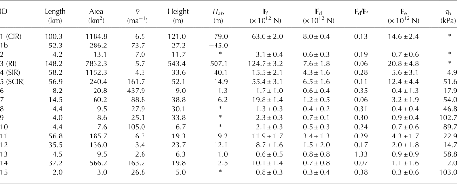
The effective resistance generated by each of the RIS pinning points can be quantified using a local force budget calculation (MacAyeal and others, Reference MacAyeal, Bindschadler, Shabtaie, Stephenson and Bentley1987). In this approach, the net traction vector acting on an imaginary contour Γ surrounding the pinning point and its associated grounded ice is partitioned into form drag and dynamic drag components estimated from observed quantities. Form drag is due to the size and shape of the obstacle within the flow field. Dynamic drag is due to the viscous deformation of the ice around the obstacle. While other approaches have been used to generate an all-encompassing buttressing parameter (Borstad and others, Reference Borstad, Rignot, Mouginot and Schodlok2013; Gudmundsson, Reference Gudmundsson2013; Fürst and others, Reference Fürst2016), our method calculates individual form drag and dynamic drag components and resolves the directional effects of the flow resistance generated by pinning points.
Form drag Ff is the glaciostatic contribution to the net resistance. Ice rises and rumples that are relatively streamlined in the flow direction generate less disturbance to the thickness field and less Ff than pinning points that are oriented transverse to flow. When the thickness of the ice shelf is uniform, Ff is zero. Ff is calculated by dividing the contour Γ around an ice rise or rumple into length elements dλ with normals  $\hat {{\bf n}}$
 $${\bf F}_{\rm f} = \oint \limits_{\rm \Gamma } {\left\{ {\displaystyle{1 \over 2}{\rho }_{i}gH^{2} + \displaystyle{{\alpha } \over {\beta }}{gH} + \displaystyle{{\alpha } \over {{\beta }^2}}{(1 - e}^{{\beta H}})g} \right\}} \hat{{\bf n}}{\rm d} {\lambda }$$
where g is acceleration due to gravity (9.81 ms−2). The second and third terms account for the lower density of the firn layer using the constants α and β from the usual depth-density relation (Cuffey and Paterson, Reference Cuffey and Paterson2010, p.19)
 $$\rho(z)=\rho_{\rm i}-\alpha\exp(\beta(z_{\rm s}-z))$$
where ρ(z) is the density at depth z, z s is the z-coordinate of the ice-shelf surface, and ρ i is the density of ice at the surface. α and β vary across the ice shelf and cannot be calculated without prior in situ measurements of the firn density profile. Values of α = 608 kg m−3 and β = −0.043 m−1 are used here (MacAyeal and others, Reference MacAyeal, Bindschadler, Shabtaie, Stephenson and Bentley1987).
Dynamic drag Fd is the viscous resistance associated with ice deformation around an ice rise or rumple. Fd reaches a maximum when ice velocity around a pinning point reduces to zero. It is calculated around the contour surrounding the obstacle
 $${\bf F}_{\rm d}=-\oint \limits_\Gamma 2{\bar v}^{z}H\left\{ {\dot \epsilon}_{ij}\cdot {\hat {\bf n}}+({\dot \epsilon}_{xx}+{\dot \epsilon}_{yy}){\hat {\bf n}}\right\} {\rm d}\lambda$$
where  $\bar {v}^{z}$ is the effective depth-averaged viscosity and $\dot {\epsilon }_{ij}$ is the strain rate tensor. The effective viscosity parameter $\bar {v}^{z}$ is
 $$\bar v^z = \displaystyle{{\bar B} \over {2{\dot \epsilon }_e^{1 - 1/n} }}$$
where  $\bar {B}$ is the depth-average, inverse flow-law rate constant and n = 3 is the flow-law exponent. The effective strain rate $\dot {\epsilon }_{e}$ is the second invariant of the strain rate tensor
 $${\dot \epsilon}{^{2}_{e}} = {\displaystyle{1}\over{2}} \left({\dot \epsilon}{^{2}_{xx}}+{\dot \epsilon}{^{2}_{yy}}+{\dot \epsilon}{^{2}_{zz}}\right)+{\dot \epsilon}{^{2}_{xy}}+{\dot \epsilon}{^{2}_{xz}}+{\dot \epsilon}{^{2}_{yz}}.$$
The local significance of Ff and Fd can be assessed by calculating the imaginary resistive force that would exist at the same location on the ice shelf, but in the absence of the pinning point. In this situation, the region contained within the contour Γ consists only of floating ice shelf with the pinning point replaced by seawater. The force transmitted through Γ is the seawater pressure Fw
 $${\bf F}_{\rm w} = \oint \limits_\Gamma {\displaystyle{{1} \over {2}}} \displaystyle {{g} \over {{\rho }_{w}}}\left\{ {{\rho }_{i}{H + }\displaystyle{{\alpha } \over {\beta }}{(1} - {e}^{{\beta H}})} \right\}^{2}\hat{{\bf n}}{\rm d\lambda }.$$
The difference between (Ff + Fd) and Fw is the effective resistance Fe, the total reaction force arising from contact between the pinning point and the base of the ice shelf
 $${\bf \,F}_{\rm e} = {\bf\,F}_{\rm f} + {\bf\,F}_{\rm d} - {\bf\,F}_{\rm w}.$$
For an area of floating ice shelf free of ice rises or rumples, Fe should equal zero or fall within the uncertainty range of zero given the satellite-derived data available for this calculation. When the magnitude of Fe for an ice rumple is within the uncertainty of zero, the feature cannot be claimed to make a contribution to flow resistance.
Uncertainty in the force budget calculation arises from (1) the errors in the velocity data and strain rates calculated from velocity gradients; (2) error in the GLAS 500 m DEM and inferred ice shelf thickness; and (3) the estimated  $\bar {B}$ value (Table 1). Uncertainty in derived quantities is evaluated by adding the individual sources of error in quadrature (Taylor, Reference Taylor1997, p. 75).
Table 1. Uncertainties of variables in the force budget calculations

Application
The force budget analysis is applied to the RIS ice rises and rumples listed in Table 2. Ice rumples nearby one another (e.g., the SCIR complex, CIR and its offshore rumple #1b) are treated as a single feature contained by a single closed contour Γ. Terms in the force budget are calculated along circular or elliptical shaped contours composed of numerous smaller segments. Each contour encloses the surface features, small areas of floating ice shelf surrounding the pinning point, and any regions of crevassing originating from the ice rise or rumple. The contour boundary can be imagined as a vertical cylinder intersecting the ice shelf. The number of segments comprising each contour is scaled to the size of the ice rise or rumple.
Table 2. Mechanical inventory of pinning points in the RIS. 1 = Crary Ice Rise, 2 = Deverall Island, 3 = Roosevelt Island and 4 = Steershead Ice Rise. Pinning points 5–15 are ice rumples
Ice thickness and strain rate components must be interpolated from the gridded datasets to the polygon vertices. Two methods were tried and compared. The first method applied linear interpolation to return strain rate and thickness at each vertex. In the second method, average values were calculated within a fixed radius around each vertex. The averaging radius is varied according to the nearness of the pinning point to other grounded features. The second method was preferred because spatial averaging reduces noise in the input datasets and consequently the propagated errors in Ff and Fd are smaller. The same averaging method is applied to the ice shelf thickness data for consistency. Force budget components (Eqns (4, 6, 9)) are determined from the gridded ice thickness and strain rate data (integrals are computed in the Appendix).
When the ice runs aground to form an ice rumple, a traction arises on the plane between the two materials and this is related to the effective resistance. The apparent basal shear stress τ b is computed as the quotient of Fe and the pinning point area. The contact area is not observable so it is approximated as the surface area of the ice rumple.
RESULTS
Inventory of RIS pinning points
The flow-modifying effects of the RIS pinning points span two orders of magnitude in Fe (Fig. 2, Table 2). In general, large ice rises (RI, CIR, SIR) generate a larger Fe than the smaller-scale ice rumples. However, the SCIR generate Fe comparable with the Fe generated by RI and CIR, and approximately double the Fe generated by SIR. In general, Fe is oriented upstream along the long axis of the ice rise or rumple. CIR and RI are a notable exception to this. These ice rises and the SCIR are discussed in more detail below.

Fig. 2. Ross Ice Shelf thickness and the effective resistance Fe generated by each pinning point. Ice thickness (m) is computed from the GLAS 500 m surface elevation model (DiMarzio, Reference DiMarzio2007) and a firn correction map (Le Brocq and others, Reference Le Brocq, Payne and Vieli2010), and overlayed onto the MODIS MOA (Haran and others, Reference Haran, Bohlander, Scambos, Painter and Fahnestock2014). The white line represents the grounding zone (Bindschadler and others, Reference Bindschadler2011).
The relative contributions of Ff and Fd to ice flow resistance also vary across the different features (Table 2). For almost all of the pinning points, Ff is the dominant term in the force budget. Ff is associated with relative compression and thickening upstream and relative extension and thinning downstream of an obstacle. Unsurprisingly, larger ice rises generate larger Ff, except for SIR. The ratio Fd : Ff is larger for ice rumples than for ice rises by approximately one order of magnitude. Using this metric as a criterion, SIR is classified as an ice rumple rather than an ice rise, even though velocity over the grounded area is very low. SIR generates significant disruption to the surrounding ice deformation field and therefore has a larger Fd : Ff ratio.
The SCIR
The SCIR are located approximately halfway between RI and the outlet of MacAyeal Ice Stream (MacIS). The ice rumples have an irregular, undulating topography and are approximately oriented in the direction of ice flow, but are not streamlined. Wakes of heavily crevassed ice extend downstream from the two largest rumples for ~20 km (Fig. 3a). Several distinct features comprise the rumple complex. The largest has an area of 78 km2 while the smallest has an area of just 4 km2. Collectively, the rumples extend over an area of 240 km2 (1400 km2 inclusive of floating ice between the pinning points). Individual rumples are relatively small features, but all together the rumple complex generates a large Fe (Fig. 2).

Fig. 3. The SCIR: (a) Surface morphology and crevasse patterns. The panchromatic image is from Landsat 8, Path 021 Row 118, acquired on 3 February 2016. (b) Shear strain rate in a flow-following coordinate system computed using the Landsat 8 velocity data.
Ice flowing over the pinning points originates from MacIS. Ice speed decreases from 400 ma−1 as ice approaches the rumpled region, to 200 ma−1 immediately downstream (Fig. 1). The ice rumples support thicker ice upstream (H = 730 m), and thinner ice downstream (H = 520 m) and divert faster ice flow from MacIS around the western shore of RI (Figs 1 and 2). This redirection also increases the ice shelf thickness downstream of Bindschadler Ice Stream (labelled BIS in Fig. 2).
Force budgets for individual ice rumples, which can be inferred from the pattern of Ff and Fd vector components around the rumple complex, depend on their position relative to other rumples. Ff magnitudes along the upstream (southeast) edge of the rumples are 30% higher than Ff along the downstream (northwest) edge (Fig. 4a). The western flank also generates a slightly greater Ff than the eastern flank, associated with thicker ice to the west and thinner ice in the lee of the upstream-most rumples. Net Ff is therefore directed upstream (Fig. 4c).
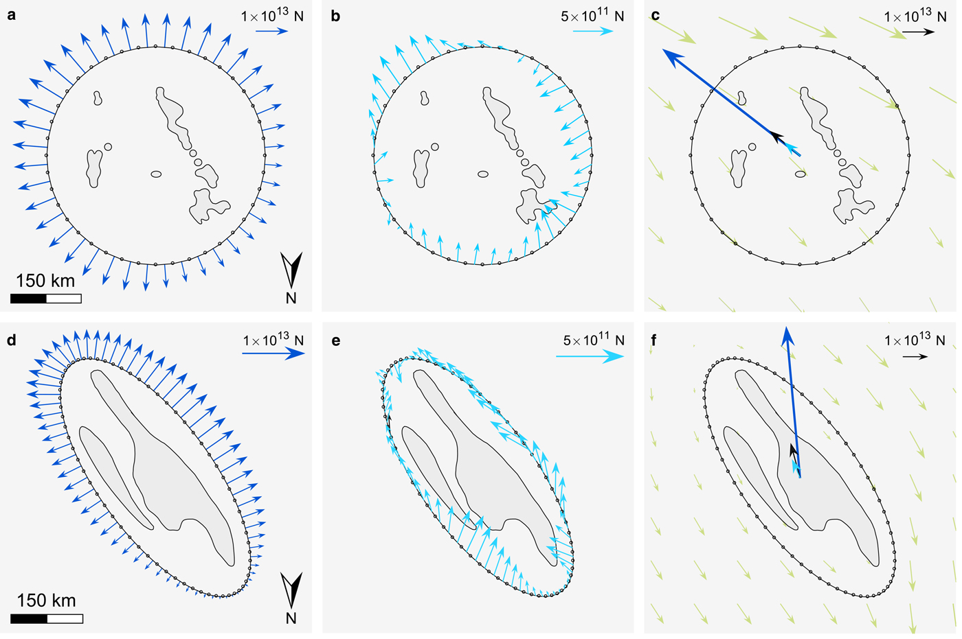
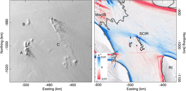
Fig. 4. SCIR and CIR force budget components. Individual Ff vector components are shown in panels (a) and (d). Fd vector components are shown in panels (b) and (e). Panels (c) and (f) show the relative magnitudes of net Ff (dark blue), net Fd (light blue) and Fe (black). Green vectors indicate the flow direction. Force budget vector components in (a), (b), (d) and (e) are scaled differently to demonstrate spatial patterns around the pinning point complexes.
The upstream and southwest flank of the ice rumple complex (labelled B and C in Fig. 3) contributes the largest Fd (Fig. 4b). The eastern rumples (labelled A in Fig. 3) are in the flow shadow of the remaining rumples and thus contribute minimal dynamic drag. Nevertheless, rumple A contributes to the overall force balance by generating compressive stresses in the upstream direction. Net Fe is directed upstream and therefore the flow regulating effect of the ice rumples is mainly on MacIS and its grounding line.
A continuous band of relatively large shear strain rates extends from the Shirase Coast, near the outlet of MacIs, to the southernmost shore of RI (Fig. 3b). This band can be seen as both a cause and consequence of the preferred ice flux direction south of the ice rumples, between Siple Dome and the SCIR. The pinning points modify the force budget by creating a band of shearing diverted away from the coast. This, in turn, favours thicker ice and faster flow south of the rumples and continued shearing reinforces this pattern. It also reduces mass flux to the north, resulting in relatively thinner ice between RI and the coast.
The SCIR have two further effects on the wider RIS. First, thinning downstream of the rumples results in a thickness gradient around RI that is not oriented along flow. As a result, RI's force budget is characterised by a relatively large Fe oriented 40° against the direction of flow, toward Siple Dome (Fig. 2). Second, ice flow downstream of the BIS grounding line is relatively thick due to MacIS flow diversion around the SCIR, generating larger flow buttressing (Fürst and others, Reference Fürst2016) than would be the case for thinner ice.
CIR
Unlike the SCIR, CIR is a demonstrably long-lived feature that is unlikely to experience changes in morphology or extent of grounding over the coming decades. The formation of CIR began with ice freezing on the bed at the southern (upstream) end 1100 years ago and the northern end stagnating 500 years later (Bindschadler and others, Reference Bindschadler, Roberts and Iken1990). Ice stream discharge around the ice rise has been variable since that time (Hulbe and Fahnestock, Reference Hulbe and Fahnestock2007) and recently, flow across the lightly-grounded ice plain upstream of CIR has slowed (Joughin and others, Reference Joughin2005; Winberry and others, Reference Winberry, Anandakrishnan, Alley, Wiens and Pratt2014). Ice thickness around CIR has also changed over time as a result of its stagnation and changes in the flux of ice from upstream (Hulbe and others, Reference Hulbe, Scambos, Lee, Bohlander and Haran2013; Fried and others, Reference Fried, Hulbe and Fahnestock2014).
CIR consists of a prominent dome rising ~100 m above the ice surface along an 80 km ridge aligned with the direction of ice flow. The southernmost tip of the CIR ridge intersects the Whillans Ice Stream (WIS) ice plain and ice flow diverges around the grounded feature. Shearing between the stagnant ice of CIR and the much faster-flowing ice stream and ice shelf creates narrow crevassed margins and a wake of extensive crevassing extending 100 km downstream. A large ice rumple (#1b in Fig. 1), off the eastern shore of CIR, is also aligned in the flow direction. Several very small features near the grounding line south of CIR are apparent in the MOA and the GLAS 500 m DEM. CIR and the large ice rumple are treated as a single feature for the force budget analysis. Of all the pinning points in the RIS, CIR generates the second largest Fe (14.6 ± 2.4 × 10¹² N).
Several smaller, potential pinning points around CIR appear as changes in surface texture but are not associated with changes in velocity. The larger feature east of CIR (#1b in Fig. 1) was described by Bindschadler and others (Reference Bindschadler1988) as an ‘ice raft’, or a block of crevasse free ice with regular internal layers, detached from CIR and moving with the surrounding ice flow. Its most recently measured speed is 73 ma−1 (Fig. 1), while Bindschadler and others (Reference Bindschadler1988) reported a speed of 140 ma−1. Ice rumple #1b rises 27 m above the surrounding ice surface (Table 2) however, the resolution of the Bedmap2 bed elevation is not fine enough to determine whether the ice runs aground at this site.
CIR modifies flow velocity and ice thickness in the region (Figs 1 and 2). Upstream, ice speed decelerates from 300 ma−1 to nearly 0 ma−1 over a distance of 70 km. Net Fd is oriented upstream in the direction of the long axis of the ice rise (Fig. 4f). The RIS is relatively thicker on the western side of CIR because ice flow is constricted between the ice rise and the Transantarctic Mountains. This arrangement influences the alignment of the net Ff vector. Rather than alignment with the flow direction, Ff and Fe are aligned 30° against the direction of ice shelf flow, towards the Transantarctic Mountains (Fig. 2). Through its effect on regional ice thickness, the ice rise thus affects the force budgets of multiple ice stream and glacier grounding lines.
DISCUSSION
Pinning points modify the force and mass budgets of ice shelves. Where the ice runs aground, a new resistive force is generated and the driving force must become larger to overcome the additional resistive force. Thickening upstream generates the additional driving force. Expressed another way, strain rates are modified where the ice runs aground, with relative compression upstream, shear along the margins of the obstacle and extension downstream. The resulting change in ice flux generates thickening upstream and thinning downstream of the pinning point. The net effects are captured in our calculation of Ff and Fd.
The ratio Fd : Ff indicates the relative importance of the resistive forces generated by individual features. The SCIR, CIR, RI and the unnamed ice rumples #7 and #14, have similar, relatively small, Fd : Ff (Table 2). Their influence on the ice thickness field thus appears to be relatively more important to the force budget than for other pinning points. The group of ice rumples downstream of Siple Dome (SIR, #11, #12, #13) all have relatively high Fd : Ff. They are located in a region of relatively slow flow, yet they have a relatively larger influence on the velocity field than other pinning points.
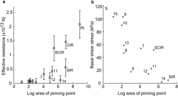
The range of Fe cannot be explained by either pinning point area A or location in the flow field alone (Fig. 5a). For example, the relatively small SCIR are responsible for a relatively large Fe while the much larger ice rumple #14 generates a much smaller Fe (12.4 ± 4.4 × 10¹² N vs. 1.1 ± 1.6 × 10¹² N, respectively). Both rumples are in relatively fast-flowing areas of the ice shelf, and both are characterised by similar, low, H ab. Including the point (0,0), the equation for the best fit linear regression line is Fe = 2.97 × 10⁶ A with  $R^2 = 0.46 \; \left(p \lt 0.01,\, \alpha = 0.05\right)$.

Fig. 5. Pinning point area vs. (a) effective resistance Fe and (b) basal shear stress τ b.
Dividing the effective resistance by the area of an ice rumple gives the apparent basal shear stress τ b (Fig. 5b). The magnitudes of τ b computed here are similar to values computed for ice stream sticky spots (τ b = 20 to 100+ kPa) (MacAyeal and others, Reference MacAyeal, Bindschadler and Scambos1995; Joughin and others, Reference Joughin, MacAyeal and Tulaczyk2004). It is possible that the range of τ b values arises from the characteristics of the subglacial material (Bougamont and others, Reference Bougamont, Tulaczyk and Joughin2003; Iverson, Reference Iverson2010). Large rumples with relatively uniform surface elevation and smaller τ b may be underlain by softer sediments. Small features with large τ b may be grounded on bedrock rather than softer sediment. Differences in τ b across different ice stream outlet regions may reflect a difference in till geology and so, for example, we might surmise that the subglacial materials beneath the SCIR complex (τ b = 51.6 kPa) and ice rumple #14 (τ b = 2.0 kPa) differ.
Our force budget results for CIR are in agreement with the original force budget analysis of MacAyeal and others (Reference MacAyeal, Bindschadler, Shabtaie, Stephenson and Bentley1987, Reference MacAyeal, Bindschadler, Stephenson, Shabtaie and Bentley1989). While we calculate a smaller Fe (1.4 ± 0.2 × 10¹³ N vs. 2.26 ± 0.07 × 10¹³ N), the oblique direction of the Fe vector is almost identical to the direction of Fe calculated by MacAyeal and others (Reference MacAyeal, Bindschadler, Shabtaie, Stephenson and Bentley1987, Reference MacAyeal, Bindschadler, Stephenson, Shabtaie and Bentley1989). Our smaller Fe can be attributed to changes in the flow field around CIR. Over the last four decades, the WIS ice plain has decelerated (Joughin and others, Reference Joughin2005; Winberry and others, Reference Winberry, Anandakrishnan, Alley, Wiens and Pratt2014), potentially modifying the resistive effect of CIR on the grounding line. However, the higher data density in the present analysis, resulting in a finer spatial resolution of strain rates around CIR, may be partly responsible for the different magnitudes.
Bathymetric data for ocean cavities beneath ice shelves are often insufficient to resolve topographic rises beneath ice rises and rumples (e.g., Fürst and others, Reference Fürst2015; Berger and others, Reference Berger, Favier, Drews, Derwael and Pattyn2016). The Bedmap2 sub-shelf bathymetry does not resolve regions of elevated topography beneath the smallest ice rises and rumples examined here. Other features are sparsely sampled and seafloor elevation is interpolated over tens of kilometres. In particular, the bathymetry beneath the SCIR is represented by only four measurement points obtained by radio-echo sounding (Fretwell and others, Reference Fretwell2013). Nevertheless, ice surface morphology indicates their presence and the force budget analysis conducted here indicates their importance. Failing to resolve the large Fe generated by some relatively small features could have large consequences in an ice-sheet model (Favier and others, Reference Favier, Pattyn, Berger and Drews2016; Reese and others, Reference Reese, Gudmundsson, Levermann and Winkelmann2018).
CONCLUSIONS
Using a force budget approach, we quantified the magnitude and direction of drag forces generated by 15 pinning points and pinning point complexes within the RIS. Several of these features generate a large effective resistance and have far-ranging, regional effects (SCIR, RI, CIR, SIR). For other features (e.g., ice rumples #7, #11, #12, #14), the analysis indicates a small resistive effect upstream. The magnitude of the effective resistance does not necessarily depend on the area of the pinning point, the degree of groundedness (height above buoyancy), or the classification of the feature as an ice rise or rumple. Variations in the subglacial material also appear to play an important role in determining the effective resistance generated by each feature.
Pinning points that generate a large effective resistance (CIR, RI, SCIR) have clear upstream effects transverse to flow in addition to their direct upstream effects. Upstream, pinning points cause relative compression which slows the flow and thickens ice. Mass flux is redirected around each obstacle, causing thickening laterally. This may, as at CIR, result in a net effective resistance directed oblique to the flow direction across the grounding line. CIR thus buttresses the southern part of the WIS grounding line, the Mercer Ice Stream grounding line, and part of the Transantarctic Mountains coast. Mass flux redirection around the SCIR also generates regional thickening but here the resistive force is directed along flow.
Of all the RIS pinning points, the SCIR are remarkable for generating a large effective resistance despite a relatively small collective area and low degree of groundedness (H ab ~15 m). Net effective resistance generated by the SCIR is aligned in the upstream direction and the rumples, therefore, regulate the flow of MacIS and its grounding line. A band of large shear strain rates originating from the upstream edge of the SCIR separates the thicker and faster flow south of the SCIR from the region of reduced mass flux directly downstream from the SCIR. In other words, the SCIR also modify the force budget by creating an effective shear margin, which in turn modifies the thickness gradients across the eastern sector of the RIS. As the effective shear margin is associated with the diversion of mass flux from MacIS, ice is thicker than it would otherwise be downstream of BIS. This thicker ice is an indirect effect of the SCIR and generates additional flow buttressing. Even though the net effective resistance generated by the SCIR is directed upstream, additional mechanical effects extend their influence laterally.
The SCIR play a larger role in the RIS force budget than their morphology alone would suggest. Changes in the geometries of the crevasse trains downstream of the pinning points indicate that their surface morphology and/or degree of groundedness has changed in the recent past. The average height above buoyancy for the SCIR is ~15 m so only modest thinning is required for the ice shelf to detach from the sea floor. Feedbacks involving bed roughness, ice deformation and basal melt may also be important, given the inferred bed properties (hard bedrock rather than soft sediment) here. A natural progression of this work is to simulate ice shelf flow in the presence and absence of the SCIR.
ACKNOWLEDGEMENTS
This work was supported by the New Zealand Post Antarctic Scholarship and the New Zealand Antarctic Research Institute (NZARI) funded Aotearoa New Zealand Ross Ice Shelf Programme, ‘Vulnerability of the Ross Ice Shelf in a Warming World’. We thank the editor and three reviewers for comments that helped us to improve the manuscript.
APPENDIX
The integrals in the force budget analysis (Eqns (4, 6 and 9)) are computed as follows
 $$\eqalign{&{\bf F}_{\rm f} = \sum\limits_{{\,j = 1}}^{N} {\displaystyle{{1} \over {2}}} {\Delta }{\lambda }_{\,j} {\hat{\bf n}}_{\,j} \cr & \quad \left\{ {\displaystyle{{1} \over {2}}{\rho }_{i}{g(H}_{1}^{2} + {H}_{2}^{2} ) + \displaystyle{{ \alpha } \over {\beta }}{g(H_1 + H_2})} + \displaystyle{{\alpha } \over {{\beta }^{2}}}{g(2 - e^{{\beta H}_{1}}- {e}^{{\beta }{H}_{2}})} \right\},}$$
 $$\eqalign{{\bf F}_{\rm d} = & -\sum\limits_{\,j=1}^{N} {\displaystyle{1}\over{2}}\Delta\lambda_{\,j} \left\{\left[ 2{\bar v}_{1}^{z}H_{1}({\dot \epsilon}_{1}\cdot {\hat{\bf n}}_{\,j}+({\dot \epsilon}_{xx}+{\dot \epsilon}_{yy})_{1}{\hat{\bf n}}_{\,j})\right]\right. \cr & \left. + \left[ 2\bar{v}_{2}^{z}H_{2}({\dot \epsilon}_{2}\cdot {\hat{\bf n}}_{\,j}+({\dot \epsilon}_{xx}+{\dot \epsilon}_{yy})_{2}{\hat{\bf n}}_{\,j})\right] \right\}}$$
and
 $$\eqalign{&{\bf F}_{\rm w} = \sum\limits_{{\,j = 1}}^{N} {\displaystyle{{{g \Delta }{\lambda }_{\,j}} \over {{2}{\rho }_{\rm w}}}} { \hat {\bf n}}_{\,j} \left[\displaystyle{{{\rho }_{i}^{2} } \over {3}}\left( {{H}_{2}^{2} + {H}_{1}{H}_{2} + H_{1}^{2} } \right) \right.\cr & \left. + \,{\displaystyle {2\alpha \rho_{i}} \over {\beta (H_2 - H_{1})}} \left({\displaystyle{1}\over{2}} \left(H_2^2 \, - \, H_{1}^2 \right) - e^{\beta H_2}{\displaystyle{\beta H_2 - 1}\over{\beta^2}} \, + \, e^{\beta H_{1}}{\displaystyle{\beta H_{1} - 1}\over{\beta^2}} \right) \right.\cr & \left. \,+ {\displaystyle{\alpha^2}\over{\beta (H_2 - H_{1})}} \left(\!\!\!\!H_2 - H_{1} - {\displaystyle{2}\over{\beta}} e^{\beta H_2} - {\displaystyle{2}\over{\beta}} e^{\beta H_{1}} + {\displaystyle{1}\over{2 \beta}} e^{2\beta H_2} -\, {\displaystyle{1}\over{2 \beta}} e^{2\beta H_{1}} \!\!\!\!\! \right) \!\!\! \right ] \! \! .}$$
A contour comprises N segments with the subscript j denoting the segment number. Subscripts 1 and 2 denote quantities at the start and endpoint of the jth segment, respectively.


 Open access