


1. Introduction
Surfce temperature (Ts) is a climatic “integrator” of the radiation and energy budgets at the Earth's surface. in Antarctica the Ii field is closely linked to elevation, the strength of the near-surface katabatic winds, and also the circulation in the free atmosphere (Reference PhillpotPhillpot, 1991; Reference Radok and BrownRadok and Brown, 1996) . Seasonal and interannual anomalies of Antarctic Ts are at least partly a function of the broadscale atmospheric circulation of higher southern latitudes (Reference RogersRogers, 1983), including the El Nino-Southern Oscillation (ENSO; Reference Smith and StearnsSmith and Stearns, 1993).
At stations in coastal Antarctica, the Ts tends to be negatively correlated with the “local” extent and duration of the sea ice on seasonal and longer time-scales (e.g. Reference JackaJacka, 1990; Weathcrly and others, 1991). Thus, the sea-ice record can be a proxy for temperature trends at regional and larger scales (Reference KingKing, 1994; Reference ParkinsonParkinson, 1995; Reference Jacobs and ComisoJacobs and Comiso, 1997). in the context of global climate change, reduced sea-ice extent probably exerts a positive feedback on global warming (Reference BuddBudd, 1991). Moreover, changes in the sea-ice extent influence precipitation in the Antarctic coastal zone by controlling the distance to the moisture source (Reference Bromwich and WeaverBromwich and Weaver, 1983; Reference Giovinetto, Waters and BentleyGiovinetto and others, 1990). They may also help determine the areas of, and time periods favorable for, the development of mesoscale cyclonic vortices ("mesocy-clones") over higher latitudes (Reference Fitch and CarletonFitch and Carleton, 1992; Carleton and Fitch, 1993). Mesocyclones are important in the climate of coastal Antarctica, particularly for snowfall (St ret en, 1990; Reference Rocky and BraatenRocky and Braaten, 1995), and also comprise a component of the atmospheric circumpolar trough near sea level (Reference Turner and ThomasTurner and Thomas, 1994; Carleton and Song, 1997).
The negative association between the annual-averaged station Ts and Antarctic sea-ice extent is not always statistically significant (Jacka, 1990). This implies large interannual variations, and also changes in the relative importance of factors such as the synoptic atmospheric and upper ocean circulations ι Aekley, 1981). Thus, to better evaluate the reasons behind recent Antarctic climate trends, one needs information on the interannual variability of the sea ice and its associations with temperature and the circulation (e.g. Reference HarangozoHarangozo, 1997).
This study determines the local and wider-area associations between the monthly Ts at several Antarctic automatic weather stations AWSs) and the weekly sea-ice extent in the sector 30° Ε eastward to 60° W, for the ice-growth seasons ( March-October) of 1987 89. These years exhibited considerable interannual variations in ice and temperature conditions. Satellite-based inventories of mesocyclonc activity for the South Pacific sector, developed for the two years exhibiting the most marked differences in the temperature-ice relationship (1988,1989), illustrate the link between local T„ and the larger-scale atmospheric circulation.
2. Data and Analysis
2.1. Aws Temperature Data
A number of AWSs have been operating in the Wilkes Land and Terre Adélie regions of East Antarctica (mostly Australian ones), and the Ross Sea area (mostly American ones), since the early to mid-1980s. Seven of these (Manuela, Martha-2, Whitlock, D-10, Law Dome, GF08 and GE03), plus Uranus Glacier on the Antarctic Peninsula, are used here because of their wide spatial distribution (Fig. 1). Also, their length of operation is sufficient to generate “long-term” temperature means from which individual month depar-tures can be calculated. Aspects of the AWS climatology are given in Stearns and Wendler (1988) and Reference Allison, Wendler and RadokAllison and others (1993).

Fig. 1. Location map showing theseven Fast Antarctic AWSs, plus that at Uranus Glacier, and the ten longitude sectorsfor which sea-ice extent statistics were computed.
Daily averages of Ts(°C) are computed from the 3 hourly data acquired by the U.S. AWSs in theTerre Adclie, Ross Sea and Bellingshausen Sea areas, and by the Australian AWSs in East Antarctica (Fig. 1), for the 1987-89 ice-growth seasons. For comparison with the sca-ice extent variations, a set of time-integrated temperature indices is developed for each AWS along the lines shown by Carleton and Fitch (1993) for the Ross Sea. Two indices noted to be particularly useful in that analysis are emphasized here. These are:
-
(1) the mean monthly temperature at each AWS for each of the three years (1987-89);
-
(2) the mean departure of the daily temperature from the “long-term” monthly mean at each AWS, in each year (1987-89).
The interrelationships of the temperature indices between AWSs for each year and also for the full 3 year period are determined by correlation, as are the AWS temperature associations with the sea-ice extent data.
2.2. Sea-Ice Extent Data
The latitude location of the sea-ice edge comprises one possible measure of Antarctic sea-ice conditions (cf. Parkinson, 1994; Reference GloersenGloersen, 1995; Harangozo, 1997). It is determined for the 1 April—30 September period of each year (1987 89) using weekly analyses of the US. Navy—National Oceanic and Atmospheric Administration Joint Ice Center. These analyses utilize all available conventional and satellite data, and have been used in many studies of sca-ice—atmosphere interaction (e.g. Carleton, 1983; Jacka, 1990). The weekly ice-edge latitude is obtained by averaging over 10° longitude intervals. Averages of the sea-ice extent are then computed for ten sectors of variable size, comprising the entire 30° E-60° wportion of the hemisphere (Fig. 1). The sectors, some of which partly overlap, are differentiated on the basis of their characteristic regional ice regimes documented in previous studies (e.g. Streten and Pike, 1980; Reference AckleyAckley, 1981; Cavalicri and Parkinson, 1981).
Standard bivariate correlation analysis (e.g. between ice extent and Ts) and the computation of statistical significance require data that are independent (i.e. not temporally autocorrelaled). To make negligible the persistence in the sea-ice series, which is of the order of 12 weeks for most regions (Carleton, 1989), we compute “first differences” by subtracting the ice-extent latitudes at the beginning of each month from those at the end of the month, for each longitude sector and for each month in the 3 year study period.
3. Results and Discussion
3.1. Antarctic Sea-Ice Conditions, 1987-89
The zonally averaged (30° E-60° wsector) weekly ice extents for the April September periods of 1987 89 (not shown) reveal stronger interannual differences in the second half of the season. For example, the greatest ice extent in 1987 is recorded in early August, compared with early to mid-September in the other two years. Moreover, there is a difference in the zonally averaged latitude at maximum extent of about 0.5° between the year of greatest ice (1987) and that with the least (1988). These variations are likely to be related, at least in part, to the shift from an ENSO “warm” to a “cold” event between 1987 and 1988 (Carleton, 1988; Gloersen, 1995; Reference Simmonds and JackaSimmonds and Jacka, 1995).
The inter-monthly and interannual differences in ice extent are most evident when considered by longitude (not shown), since the effects of differential ice growth and ad-vection between sectors become apparent (e.g. Jacka, 1990; Parkinson, 1991). The 1989 season had strong (weak) equa-torward ice-advance patterns in the sector from 150” Ε eastward to the Antarctic Peninsula (100° Ε eastward to 140° F). Longitudinal differences in the ice-advance patterns are much less evident in both 1987 and 1988. Ice-growth in the sector 30 90 F is broadly comparable across all three years.
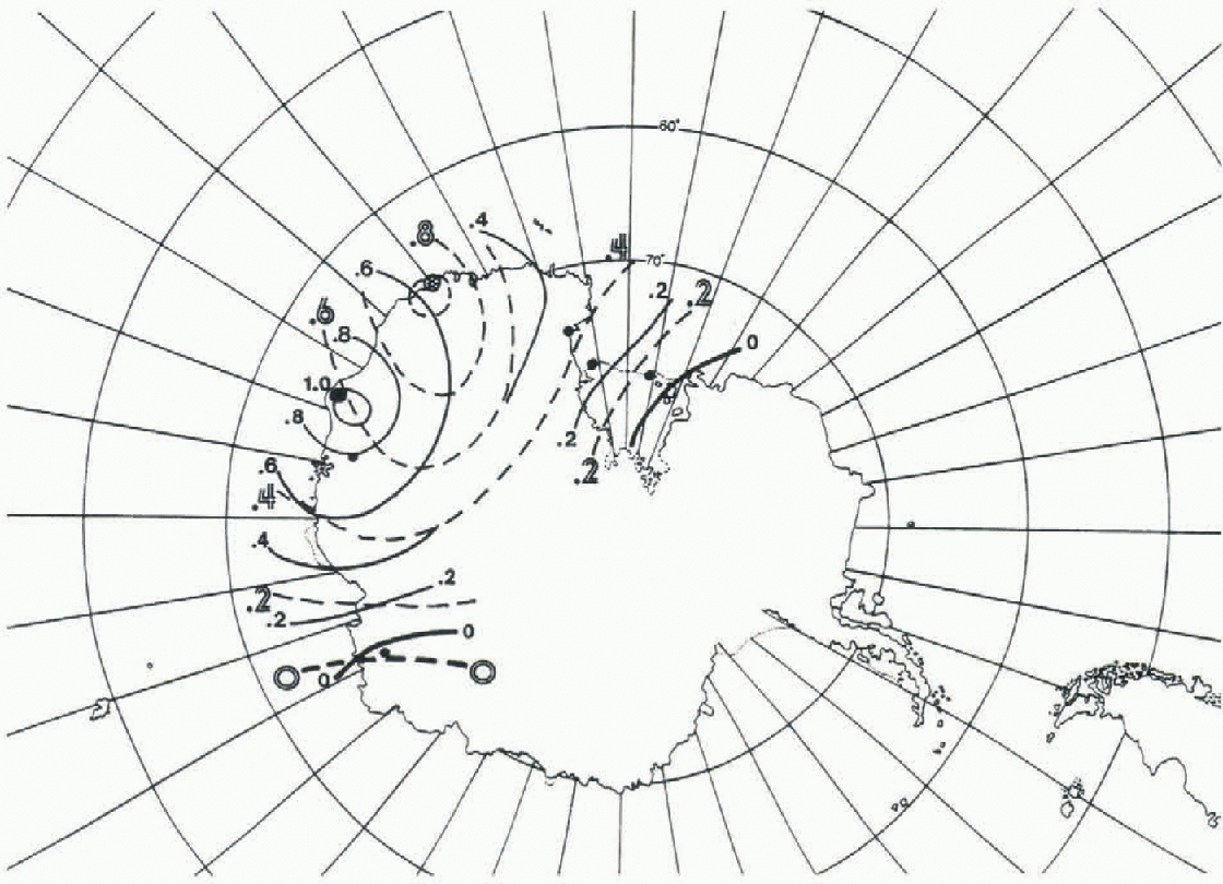
Fig. 2. Spatial patterns of the correlation between the mean temperature anomaly for the March-October period of1987-89 at Law Dome (D-10) correlated with the other AWSs: solid isolines (dashed isolines).
Intercorrelations of the monthly ice-extent changes among longitude sectors for each of the three years (1987— 89) reveal that significant correlations are almost always positive, and they tend to occur more for adjacent and partly overlapping sectors than for those more distant. However, some long-range significant ice correlations were found, for example in 1987 between 50-90°Ε and 120-60° w(r = 0.790) and between 100° Ε 180° and 90-60° w(r = 0.865). The number of significant ice intcrcorrclations varies over the three years, in 1988 being about half that of either 1987 or 1989. A similar interannual variation is evident in the intercorrelations of AWS temperatures (below).
3.2 Antarctic AWS temperature associations, 1987-89
Correlation matrices of the AWS monthly mean Ts and its anomalies give consistent results in terms of the sign and also number of significant inter-station correlations. All significant correlations are positive, confirming the more-or-less zonal symmetry of temperature anomalies for Antarctica outside the Peninsula region (Rogers, 1983). There is also a spatial decay evident in the correlations, whereby stations closer to each other tend to be more highly correlated. Stations D-10 and Law Dome tend to be better correlated with the other stations used here than are GE03 or Uranus Glacier (Fig. 2).These correlation spatial patterns were used as a basis for regionalizing (grouping) stations for the ice-temperature portion of the study, below. The four groups are Adélie/Wilkes (three stations: D-10, Law, GF08), the Ross Sea (three stations: Manuela, Martha andWhitlock), GE03 and Uranus Glacier.
There are considerable interannual variations in the number of significant intercorrelations of AWS Ts, especially for 1988 (fewest: italicized values, Table 1) and 1989 (most: non-italicized values, Table 1), and therefore also in the spatial dependence of the temperature patterns. These may be related to ENSO. For example, Reference Savage, Stearns and WeidnerSavage and others (1988) showed that the 1988 winter was unusually cold in Antarctica and followed the minimum in the Southern Oscillation Index (SOI) in 1987. This feature is consistent with the composite pattern for such ev ents shown by Smith and Stearns (1993).
3.3. Sea-Ice-Temperature Correlations, 1987-89
Table 1. Intercorrelations of AWS monthly mean temperatures for ice-growth seasons 1988 and 1989

Correlation matrices (not shown) of station Ts (individual, grouped) and the sectoral sea-ice latitude monthly change reveal the following major features:
-
(1) the greatest number of significant correlations tends to occur in the sector from about 170°Ε to 60 W, followed by the sector 30-90°E;
-
(2) despite the generally positive spatial intercorrelations of AWS Ts and sectoral ice conditions when the three years are grouped together, both negative and positive correlations occur on an individual year basis. Here, positive coefficients imply cither more ice (i.e. decreasing ice-edge latitude) and lower temperatures, or less ice (i.e. increasing ice-edge latitude) and higher temperatures.
Negative coefficients imply the opposite in each case. Moreover, there is a consistent change over the three years in the relative frequencies of significant Ts-ice-extent correlations: from mostly negative in 1987 to mostly positive in 1989. This suggests changes in the relative importance of meridional flow for advecting the temperature anomalies into the sea-ice zone (Haran-gozo, 1997), which need to be studied further. This circulation feature may also be related to the SOI variations occurring during the 1987-89 period;
-
(3) the lack of consistency in the Ts sea-ice correlations between years is especially apparent for 1988 and 1989. For example, at station GF03 correlations are weak and longitudinally restricted (strong and widespread) in 1988 (1989), even though the correlation of Ts at GE03 with Other AWSs is negligible in both years (fig. 3a and b).These results confirm the reduced spatial consistency of both the AWS Ts and sea-ice conditions in 1988.
The role of Ts in influencing the strong differences in sea-ice extent occurring between the Ross and Amundsen/ Bellingshausen Seas for the 1988 and 1989 seasons is quantified through a measure of the longitudinal gradient of AWS temperature across the Ross Ice Shelf. This is a key site for katabatic Outflows and their involvement in mesoscale cyclogenesis (e.g. Bromwich, 1991; Reference Carrasco and BromwichCarrasco and Bromwich, 1994). Here, the daily Ts departure data for Manuela are subtracted from those at Martha-2 for each ice-growth season. Thus, positive (negative) differences in the index are associated with northerly (southerly) “thermal” wind in the boundary layer for this region. figure 4a and b show that, for much of the ice-growth season of 1988 (1989), mild northerly (cold southerly) “thermal” winds predominated in the central and western Ross Sea. These accompanied the smaller (greater) increases in ice extent in those longitudes during the 1988 (1989) season, and are consistent with a larger-scale circulation pattern of a weakened (strengthened) Amundsen Sea “mean” low in 1988 (1989) (Carleton and Fitch, 1993, Fig. 8). The latter comprises part of the ENSO signal in the Antarctic (Reference Cullather, Bromwich and van WoertCullather and others, 1996).
These differences in Ts, ice conditions and atmospheric circulation are also rellected in the considerably greater frequencies of cold-air mesocyclones observed in longitudes of the eastern Ross Sea and Amundsen Sea in 1989 contrasted with 1988 (see Carleton and Fitch, 1993, Ggs 6 and 7).

Fig. 3. Maps showing the intercorrelations of mean monthly temperatures of GE03 with the sea-ice latitude monthly change for each ice sector in 1989 (a) and 1988 (b). Also shown are the correlations of Ts at GE03 and at the other AWSs for each season.

Fig. 4. Time plots of the mean daily temperature departures between Martha-2 and Manuela (cf. Fig. 1) for ice-growth seasons 1988 (a) and 1989 (b). Note the large between-year differences for the period May August.
4. Summary and Conclusions
A statistical analysis of the relationship between near-coastal Τs and Antarctic sca-ice extent for the 30° E-60° Wsector has been undertaken individually for three ice-growth seasons characterized by large interannual variations of atmospheric circulation (1987-89). While a temperaturc-sca-icc relationship that involves greater (reduced) ice extent when temperatures decrease (increase) is evident both locally and sometimes over long distances, there are strong interannual changes in the magnitude, spatial homogeneity and even sign of the association. These results likely emphasize the variable role of the atmospheric circulation for advecting temperature anomalies with in the sea-ice zone, and their larger-scale teleconncction with ENSO. They imply the need to examine the temperature-ice relationship for additional years having large variations of Antarctic circulation climate.
Acknowledgements
This research was supported by U.S. National Science Foundation Office of Polar Programs (OPP) grants 88-16912 and 92-19446. Wc are grateful to I. Allison and C. Stearns for supplying the data from the Australian and U.S. AWSs, respectively.


