1. Introduction
The present mass balance of the Antarctic ice sheet is not well known, and large uncertainties exist in its contribution to current and future sea-level rise, which is a significant concern. Current knowledge indicates that the West Antarctic ice sheet (WAIS) exhibits a bimodal behavior, thickening in the south along the Siple Coast ice streams (Reference ThomasThomas, 1976; Reference Joughin and TulaczykJoughin and Tulaczyk, 2002) and thinning in the north along the Amundsen Sea coast (Reference Shepherd, Wingham, Mansley and CorrShepherd and others, 2001), but thinning overall (Reference Rignot and ThomasRignot and Thomas, 2002). In East Antarctica, significant uncertainties of the past have been removed with the availability of new data from satellites. For instance, the large positive balances of the Lambert, Shirase and Jutulstraumen glaciers have been reduced to zero or negative. The mass budget of the East Antarctic ice sheet appears to be close to zero. However, even its sign cannot be determined. Significant uncertainties remain in areas furthest south, outside remote-sensing satellite coverage (Reference Rignot and ThomasRignot and Thomas, 2002).
The Pine Island Glacier (PIG)–Thwaites Glacier (THW) sector of West Antarctica has been identified as a key sector of the WAIS, theoretically prone to rapid collapse (Reference HughesHughes, 1981), drained by some of the most active ice streams in the Antarctic and lacking the more extensive buttressing ice shelves of the other large West Antarctic ice streams. Satellite remote-sensing data have revealed that the Pine Island Bay sector is rapidly changing at present and is losing mass to the ocean. Glacier grounding lines are retreating about 1 km a–1 (Reference RignotRignot, 1998, 2001). The glaciers are thinning several m a–1 (Reference Wingham, Ridout, Scharroo, Arthern and ShumWingham and others, 1998; Reference Shepherd, Wingham, Mansley and CorrShepherd and others, 2001, Reference Shepherd, Wingham and Mansley2002; Reference ZwallyZwally and others. 2002), and they are accelerating (Reference Rignot, Vaughan, Schmeltz, Dupont and MacAyealRignot and others, 2002). Their small ice shelves exhibit the highest steady-state bottom melt rates observed in the Antarctic (Reference Rignot and JacobsRignot and Jacobs, 2002), and they are currently thinning (Reference ZwallyZwally and others, 2002), perhaps due to warmer ocean temperatures (Reference Jacobs, Hellmer and JenkinsJacobs and others, 1996; Reference Jenkins, Vaughan, Jacobs, Hellmer and KeysJenkins and others, 1997).
Despite these advances in our knowledge of this sector of Antarctica, our understanding of the conditions that led to this evolution of the glaciers is hampered by a lack of basic glaciological and oceanographic data, some of which cannot be obtained by available satellite remote-sensing means and require airborne, ship and ground surveys (e.g. Reference AbdalatiAbdalati and others, 2004). Pine Island Bay is far from manned ground stations, and has a reputation for bad weather. It has not been part of a major glaciological program.
In an effort to overcome these limitations and demonstrate the feasibility of accessing this area by more direct means than satellites, Centro de Estudios Cientifícos (CECS), Chile, and NASA organized an airborne survey of Pine Island Bay in November–December 2002, which also included overflights of the Antarctic Peninsula and the Patagonia icefields. A P-3 aircraft on loan from the Armada de Chile was operated from Punta Arenas and deployed for four flights over the Amundsen Sea glaciers. Each flight provided 1.5–2 hours of data and covered 750–1000km of flight track.
In this paper, we present an analysis of the ice-thickness data collected during these surveys over the key glaciers draining ice from this sector of Antarctica. The data are combined with a vector velocity map obtained from ERS-1/-2 interferometric synthetic aperture radar (InSAR) data to revise our prior estimates of mass fluxes and the state of mass balance of the glaciers. We conclude by discussing how these data help us better characterize and understand the evolution of ice in this sector of the Antarctic.
2. Methods
2.1. Ice-thickness and elevation data
The payload onboard the P3 included the NASA/University of Kansas Ice Sounding Radar (ISR) and the NASA/Wallops Airborne Topographic Mapper (ATM). The ISR operates at 150MHz (Reference Gogineni, Chuah, Allen, Jezek and MooreGogineni and others, 1998, Reference Gogineni2001). Global positioning system (GPS) processing of the plane position was based on data collected by receivers mounted on the P3, Punta Arenas, Palmer and Carvajal (formely Adelaide) stations. ATM laser altimetry data and ISR ice-thickness data were successfully collected over >90% of the approximately 3500 km over-ice survey. The long GPS baseline (1400 km) resulted in an accuracy of laser-derived surface elevations of 20–30 cm, or a factor two to three lower than that achieved during overflights of the Greenland ice sheet (Reference KrabillKrabill and others, 2000).
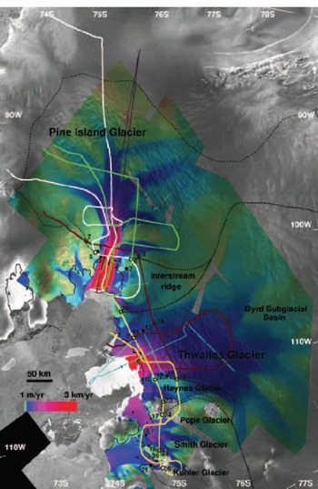
The four flights over Pine Island Bay are shown in Figure 1, overlaid on a mosaic of radar brightness from RADARSAT-1 and a velocity map from ERS-1/-2. The CECS/NASA flights were designed to capture essential glacier features such as transverse and longitudinal profiles near grounding lines, follow major tributaries revealed by InSAR, repeat earlier surveys and follow ICESat orbits. Although the coverage is sparse, the survey provides a major improvement in the amount of ice-thickness data available in the region (Reference Lythe and VaughanLythe and others, 2001), and represents the first laser altimetry data collection in this part of Antarctica.
Fig. 1. Velocity magnitude of the Amundsen Sea glaciers inferred from 1996 ERS-1/-2 InSAR data, overlaid on a RADARSAT-1 radar mosaic on a polar stereographic grid at 150 m spacing. Drainage basins are shown in dotted lines. The 1996 limit of tidal flexing is shown in black lines. Portions of the BAS 1981, 1998 and SPRI 1978 airborne radio-echo sounding flight tracks are shown, respectively, in light green, dark purple and light blue lines. Black filled circles along those flight-lines are located at the end-points of flux gates listed in Table 1. The four CECS/NASA flights, represented as thick lines, are colored, respectively, brown (28 November 2002), white (12 April 2002), green (12 June 2002) and yellow (12 December 2002). Black open circles along those four flight-lines are located at the end-points of flux gates discussed in the text and listed in Table 1 and 2. ©Canadian Space Agency 1997; ©European Space Agency 1996.
2.2. InSAR velocity
Ascending and descending tracks of ERS-1/-2 InSAR tandem data acquired in late 1995–early 1996 were combined to produce a vector velocity mosaic (Fig. 1), assuming surface-parallel flow. Along each track, interferometric pairs were used to measure ice velocity and glacier topography independently. Topographic control was provided by a prior digital elevation model (DEM) of Antarctica (Reference Bamber and BindschadlerBamber and Bindschadler, 1997). Velocity control was provided by the presence of non-moving land sectors along the coasts (nunataks, volcanoes, ice rises, etc.) and glacier divides. Two ERS tracks acquired in 2000 were subsequently added to the mosaic to complete it in regions where ice-velocity changes between 1996 and 2000 are unlikely to be significant.
In several areas used for velocity control, precise InSAR topography was crucial for obtaining reliable zero-velocity reference since the radar interferograms have to be corrected for topography prior to being used for measuring velocity. Combination of long tracks (i.e. >500 km) helped minimize uncertainties in absolute velocity in the interior. Balance velocity was not used to control the mapping, however, since this sector is not in balance (Reference Bamber and RignotBamber and Rignot, 2002). No GPS velocity control is available, which certainly limits the precision of velocity mapping in the interior regions. On the ice shelf, InSAR velocities were corrected from ocean tides. The correction assumes a purely elastic tidal deformation of ice shelves (Reference Rignot, Buscarlet, Csathό, Gogineni, Krabill and SchmeltzRignot and others, 2000) and employs tidal predictions from the FES99 tidal model (Reference Lefevre, Lyard, Provost and SchramaLefevre and others, 2002).
The velocity mosaic reveals major glaciers and tributaries (Reference Stenoien and BentleyStenoien and Bentley, 2000). More than 11 tributaries coalesce to form PIG. Six of these tributaries merge in a confluence zone about 50km upstream of the grounding line. Further downstream, a slow-moving tributary enters the glacier from the south, near the grounding line. Another tributary enters the ice shelf from the south, near the PIG– THW interstream ridge. The mapping of THW, though not complete, also reveals many tributaries. The western boundary of the interstream ridge is well revealed in the velocity map, with clear margins extending several hundred km inland. Haynes Glacier is a distinct feature from the main flow of THW. Smith Glacier results from the merging of several tributaries, one of which discharges ice into Kohler Glacier. A branch of Smith Glacier subsequently discharges ice into Dotson Ice Shelf instead of Crosson Ice Shelf. PIG flows on average near the grounding line at 2.5 km a–1, THW at 2.2 km a–1, Haynes Glacier at 350 m a–1, Pope Glacier at 650 m a– 1, Smith Glacier at 500 m a–1 and Kohler
Glacier at 700 m a–1. The position of the 1996 limit of tidal flexing (Fig. 1) was obtained from InSAR differential data (accuracy 100–200 m).
3. Results
3.1. CECS/NASA thickness vs BEDMAP
Prior to the CECS/NASA survey, no data existed along Haynes, Pope, Smith and Kohler glaciers. The new data reveal that the glaciers flow along distinct, deep troughs that extend far inland. The deepest trough, with ice 2.3 km thick (Fig. 2c), corresponds to Smith Glacier, but Pope, Kohler and Haynes glaciers boast ice thicknesses several hundred meters larger than those of PIG or THW (Fig. 2a–d).
Fig. 2. Velocity magnitude (V, red), thickness (H, black) of (a) Pine Island (‘Downstream’, labels 5–6 in Fig. 1), (b) Thwaites (extension of ‘Downstream’, labels 22–10 in Fig. 1), (c) Pope/Smith/Kohler (labels 24–26 in Fig. 1, excluding western tributary of Kohler), and (d) Haynes (labels 12–23 in Fig. 1) glaciers, measured respectively with 1996 ERS-1/-2 InSAR and 2002 CECS/NASA ISR. Ice fluxes are listed in Table 1 and 2.
Most ice thicknesses measured along THW are in reasonable agreement with BEDMAP. THW has a 120 km long front, with the active part concentrated in a region 20– 30 km wide, yet ice thickness is rather uniform across the whole glacier width (Fig. 2b).
The PIG data reveal that the northern flank of the glacier and its tributaries are shallower, by a few hundred meters, than indicated in BEDMAP. In contrast, the glacier is much deeper than indicated in BEDMAP to the south (not shown in the figures). All southern tributaries flow over deep bedrock, well below sea level. Further details on the comparison of BEDMAP vs CECS/NASA are discussed in a companion paper (Reference Thomas, Rignot, Kanagaratnam, Krabill and CasassaThomas and others, 2004).
3.2. Ice fluxes
Table 1 compares earlier estimates of ice fluxes vs revised ones. Table 2 summarizes ice fluxes for larger areas, typically extending to the full width of the glaciers revealed by InSAR. Earlier flux gates were narrower because ice thickness cannot be calculated reliably from elevation data near glacier margins (rougher topography, more variable surface), and InSAR velocity mapping has since been extended in spatial coverage. The end-points of the flux gates discussed in Table 1 and 2 are labeled in Figure 1.
Table 1. Glacier fluxes (km3 ice a–1) along CECS/NASA flight-lines (end-points in parentheses indicate the position of the end-points of the flux gates in Fig. 1) vs prior fluxes calculated at the grounding line (GL)
ISR thicknesses were reduced by 12 m (e.g. Reference Jenkins and MJenkins and Doake, 1991) to convert the firn layer thickness into an ice equivalent thickness for calculation of ice volume fluxes. Distances along flux gates include a correction factor for the polar stereographic projection since this projection does not conserve distances. The uncertainty in ice velocity is 15 m a–1. The uncertainty in thickness is 15 m. The percentage error in ice flux (Table 1 and 2) is the sum of the percentage error in mean thickness and percentage error in mean velocity.
The grounding-line flux of PIG, previously estimated at 76±4 km3 a–1 (Reference RignotRignot, 1998) and revised at 75 ±3km3 a–1 with BEDMAP (Reference Rignot, Vaughan, Schmeltz, Dupont and MacAyealRignot and others, 2002), is confirmed using a profile along parallel flowlines nearest to the 1996 grounding line (Table 1; labels 3–4 in Fig. 1). The CECS/NASA data, however, permit inclusion of the full width of the glacier, including its western tributary (labels 5–6 in Fig. 1), to yield a total flux of 84.2 ±2km3 a–1 (Fig. 2a; Table 2). Across a transverse profile located further upstream (noted ‘Upstream’ in Table 1; labels 7–8 in Fig. 1), the ice flux is nearly identical. In contrast, the ice flux calculated using the British Antarctic Survey (BAS) 1981 data (Reference Crabtree and M. DoakeCrabtree and Doake, 1982) is lower (Table 1; labels 1–2 in Fig. 1), and unreliable for two reasons: (1) the positional accuracy of the data is uncertain (Reference Jenkins, Vaughan, Jacobs, Hellmer and KeysJenkins and others, 1997); (2) half of the profile is on floating ice where basal melt rates exceed 50 ma–1 (Reference RignotRignot, 1998) and hence ice discharge into the ocean is systematically underestimated.
Table 2. Glacier fluxes (km3 ice a–1) obtained combining 1996 InSAR velocities and CECS/NASA thickness vs snow accumulation. The drainage area (in km2) is indicated in parentheses in the third column. The bottom row shows the mass imbalance in 2000, assuming a 10% and 4% increase in ice discharge for PIG and THW, respectively, and no change for the other glaciers

The ice fluxes of THW calculated at the grounding line and along the Scott Polar Research Institute (SPRI) profile are not confirmed because of an error in earlier calculations of the normal vector to the flux gate (Reference RignotRignot, 2001). The correct flux is 20% larger (Table 1; labels 9–10 in Fig. 1). Along three profiles (SPRI, ‘Upstream’ and ‘Downstream’ in Table 1; labels 11–12, 13–14, and 15–16 in Fig. 1), the revised ice fluxes are within the measurement error. THW is, however, broader than suggested by these earlier flux gates. Over its full extent revealed by InSAR (labels 22–10 in Fig. 1; Fig. 2b), THW discharges 101.8±4 km3 a–1 ice (Table 2). This makes THW the largest discharger of ice in the Antarctic.
The fluxes of Pope and Smith Glaciers calculated earlier using ice thickness deduced from elevation data assuming hydrostatic equilibrium over a narrow gate (Smith/Pope 1996 GL in Table 1, and labels 17–18 and 20–21 in Fig. 1) and a large gate (Smith/Pope Extended in Table 1; and labels 24–25 in Fig. 1) agree with the revised fluxes calculated using the CECS/NASA data (Fig. 2c). Only the western branch of Kohler Glacier (labels 21–26 in Fig. 1) could not be surveyed. Its ice flux was still calculated using ice thickness deduced from the ice-shelf elevation. The total flux from these three glaciers combined (Table 2) is more than one-third of the ice flux of PIG. These glaciers therefore play an important role in the overall ice discharge from this sector. The same conclusion applies to the 8.7±1km3 a–1 discharge of Haynes Glacier, which had never been estimated before because it has no floating ice for which ice thickness can be deduced from ice-shelf elevation (the glacier calves before ice reaches hydrostatic equilibrium).
Overall, the ensemble of PIG, THW, Haynes, Pope, Smith and Kohler glaciers, combined with the region in between PIG and THW (named ‘Interstream ridge’ in Table 2 and Fig. 1) discharge 241 ±5km3 a–1 ice in 1996. If we include a correction factor for the acceleration and widening of PIG (10%) and THW (4%) (Reference Rignot, Vaughan, Schmeltz, Dupont and MacAyealRignot and others, 2002), the total flux in 2000 is 253±5km3 a–1 in 2000 (Table 2). No ERS data were acquired over Haynes/Pope/Smith/Kohler glaciers in 2000 to measure their velocity, and RADARSAT-1 data yield very low signal correlation in this region.
3.3. Mass balance
We compare the ice fluxes calculated for large sectors with snow accumulation in the interior from Reference Giovinetto and ZwallyGiovinetto and Zwally (2000) (Table 2). The drainage basins of the glaciers have been updated to reflect the selection of wider flux gates. We assume that snow accumulation is known with 10% uncertainty over these broad basins. The mass imbalances of PIG, Kohler, Smith and Pope glaciers confirm earlier estimates, but the precision of the results is improved (Reference Rignot and ThomasRignot and Thomas, 2002). The imbalance of THW is larger for the reason indicated earlier. The imbalance of Haynes Glacier and the interstream ridge region had never been estimated. Overall, the mass imbalance of this region is –81 ±17 km3 a–1 in 1996. Using an ice density of 917 kg m–3 and a 1 mm sea-level equivalent of 360 Gt, this implies a sea-level rise of 0.21 ±0.04 mm a–1 in 1996. In 2000, this contribution increased to 0.24±0.04 mm a–1. While the total mass loss is dominated by the negative mass budget of THW, the smaller glaciers are proportionally more out of balance than THW.
3.4. Grounding-line retreat
Hydrostatic equilibrium is calculated from ATM elevations corrected for geoid–ellipsoid separation using the Ohio State University (OSU) 1991 model, and using column-averaged sea-water density of 1027.5 kg m–3 and ice density of 900 kg m–3. Comparison of the OSU 91 geoid with ATM elevation on the ocean surface suggests an uncertainty of <3–4m in the geoid. The use of slightly different values of the water and ice densities does not change the location of the line of first hydrostatic equilibrium of ice by more than a few hundred meters. Prior studies conducted in Greenland indicated that the line of hydrostatic equilibrium of the ice is on average within 1 km of the InSAR-derived limit of tidal flexing (Reference Rignot, Gogineni, Joughin and KrabillRignot and others, 2001). A separation of several km between the 1996 limit of tidal flexing and the 2002 line of hydrostatic equilibrium is therefore significant.
Grounding-line retreat has already been reported for PIG in 1992–1994–1996 (Reference RignotRignot, 1998) and 2000 (Reference RignotRignot, 2002), and on THW in 1992–1994–1996 (Reference RignotRignot, 2001). As shown in Figure 3c, the 2002 limit of hydrostatic equilibrium of ice on PIG is upstream of the InSAR-derived 1996 limit of tidal flexing, which suggests that the grounding line continued its retreat in the last 7 years (early 1996–late 2002). As ice is only 20–40m above hydrostatic equilibrium in the 25 km long ice-plain region immediately upstream (Reference Corr, Doake, Jenkins and VaughanCorr and others, 2001), grounding-line retreat is likely to continue until the entire ice plain is afloat (Reference ThomasThomas and others, 2004).
Fig. 3. Along-flow thickness, H, and laser altimetry elevation, h, of (a) Pope Glacier (mission 12 December 2002), (b) Kohler Glacier (mission 12 December 2002), and (c) Pine Island Glacier (mission 4 December 2002), with bedrock profile corresponding to that expected when ice is in hydrostatic equilibrium in red. The point of departure between the measured bedrock profile and that calculated from hydrostatic equilibrium marks the limit of hydrostatic equilibrium of the ice, which is a proxy for the November– December 2002 position of the grounding line. Diamonds indicate the position of the November 1995–February 1996 limit of tidal flexing of the ice inferred from InSAR.
The grounding line of Kohler Glacier retreated a few km between 1992 and 1996 (Fig. 4). It continued its retreat through late 2002, almost 10 km inland of the 1992 position. The retreat is likely to stop in the near future because of a bedrock high immediately upstream of the present limit of flotation of the ice (Fig. 3b). Once the glacier thins sufficiently for the grounding line to retreat pass this sill, we anticipate that the grounding line will resume its rapid retreat. In contrast, the grounding line of Pope Glacier is only slightly inland of its 1996 position. This may be a temporary position as ice is only 100–200m above hydrostatic equilibrium in the 15 km long segment upstream of the 2002 grounding line (Fig. 3a).
Fig. 4. Limit of tidal flexing of Kohler, Smith and Pope glaciers measured in March 1992 (black line) and November 1995/January 1996 (blue line) with ERS-1/-2 InSAR. Zones where ice is in hydrostatic equilibrium in November–December 2002 are shown in thick red lines along the CECS/NASA flights (thin white lines). Apparently missing zones of red thick lines on the ice shelf are due to the absence of good laser altimetry data in those segments. The data are overlaid on a 1992 double-difference interferogram of the area, where each color cycle represents a 3 cm incremental vertical displacement of the ice shelf due to changes in ocean tide.
The grounding line of Smith Glacier retreated between 1992 and 1996, but not as rapidly as that of its neighbors. Yet, a survey profile acquired in 2002 shows ice to be in hydrostatic equilibrium 15 km upstream of the 1996 limit of tidal flexing, which indicates a large retreat. No ATM/ISR data were collected along the glacier flow direction, but a comparison of ice thickness inferred from the Antarctic DEM assuming hydrostatic equilibrium with CECS/NASA thickness on the ice shelf, and at the 2002 line of hydrostatic equilibrium, shows differences of <100 m. This means that this region was already close to hydrostatic equilibrium in 1994. It is likely to correspond to an ice plain, similar to the ice plain found on PIG and THW.
4. Discussion
The CECS/NASA thickness data, combined with the InSAR velocity mosaic, confirm the overall state of negative mass balance of this region (Reference Rignot and ThomasRignot and Thomas, 2002). This sector alone is contributing significantly to sea-level rise (0.21±0.04 mm a–1), and this contribution will increase in the future if the glaciers continue to accelerate. The new data also suggest that grounding lines are continuing their retreat, with retreat rates of about 1 km a–1, which implies several m a–1 thinning of the glaciers at the grounding line (Reference Shepherd, Wingham and MansleyShepherd and others, 2002; Reference ZwallyZwally and others, 2002). These thinning rates are high by Antarctic standards where near-coastal snow accumulation is 0.4 m a–1 (Table 2). As surface melting or sublimation is negligible, the most likely explanation for the thinning is enhanced flow of the ice. Indeed, the largest glaciers have been accelerating over at least the last decade (Reference Rignot, Vaughan, Schmeltz, Dupont and MacAyealRignot and others, 2002; Joughin and others, 2003; C. E. Rosanova and B. K. Lucchitta, unpublished information). Despite their smaller size and reduced flow rates, Haynes, Pope, Smith and Kohler glaciers contribute largely to the imbalance of this sector and already flow several times faster than their balance velocities.
All glacier floating sections experience high bottom melting near the grounding line because of their deep ice draft (the melting point of ice decreases with increasing water pressure, and is therefore lower for deeper ice) and because of the presence of warm ocean waters (Reference Rignot and JacobsRignot and Jacobs, 2002). Freshening of the ocean waters in the Ross Sea has been attributed in part to enhanced ice-shelf meltwater production in the Amundsen Sea (Reference Jacobs, Giulivi and MeleJacobs and others, 2002). One distinct possibility is that all the glaciers discussed herein, and perhaps other glaciers in the nearby sectors of Getz Ice Shelf, are contributing to this freshening of the ocean. Although the connection between a warmer ocean, thinning ice shelves and retreating glaciers cannot be established firmly from our data, this survey and results already gathered from satellites strongly suggest the possibility of a linkage between glacier speed-up, ice-shelf weakening and a warmer ocean. In contrast, West Antarctic glaciers not directly exposed to warm ocean waters are thickening at present (Reference Joughin and TulaczykJoughin and Tulaczyk, 2002).
5. Conclusions
The results of the CECS/NASA campaign confirm that the glaciers which drain West Antarctic ice into the Amundsen Sea are retreating rapidly and flow over very deep bedrock extending far inland. Their current contribution to sea-level rise, as estimated here, is the largest reported to date from any glaciated region in the world. The deep beds characterizing these glaciers increase the potential for coastal changes to propagate further and rapidly inland and affect a larger part of West Antarctica. There are no major bedrock sills to halt the retreat of these glaciers. The glaciers could flow considerably faster once the ice shelves have been sufficiently weakened, which in turn would increase their contribution to sea level. As part of a research effort to better understand this region, we anticipate more data collection of this nature to complete the mapping of this region and continue to monitor and understand its rapid evolution.
Acknowledgements
We thank pilots, crew members, technicians and staff from the Armada de Chile, University of Kansas, NASA/Goddard Space Flight Center (GSFC) Wallops Flight Facility and CECS who helped make the surveys over Antarctica; M. Arevalo and F. Contreras for providing logistic support in Punta Arenas; Direcciόn General de Aeronáutica Civil for office space and general support at the airport in Punta Arenas; R. Sinclair for coordination in Punta Arenas; T. Hughes for helping with planning flight routes; and BAS, the US Geological Survey, the US National Oceanic and Atmospheric Administration, Direcciόn Meterolόgica de Chile and the field team at base Carvajal for providing weather reports/forecasts and GPS data that made possible the flights and subsequent accurate trajectory calculations. We thank the scientific editor, H. Fricker, the reviewers, T. Scambos and D. Vaughan, and I. Joughin for comments on the paper. The European Space Agency and the Alaska SAR Facility are acknowledged for collecting and distributing the satellite radar data employed in this study. This work was performed at CECS through Fundaciόn Andes and the Millennium Science Initiative, and at the Jet Propulsion Laboratory, California Institute of Technology, the University of Kansas and the NASA/GSFCWallops Flight Facility under a contract with the National Aeronautics and Space Administration, Cryospheric Science Program. The overall success of our surveys owes much to the guidance and persistence of C. Teitelboim from CECS and W. Abdalati from NASA.