


Introduction
The response of ice sheets to climatic forcing is complicated and numerical models are needed to quantify the interaction between ice flow, ice-temperature field, etc. Still, no matter how accurate such a model is, the value of a particular simulation depends critically on the formulation of the surface mass balance. Recently, highly parameterized mass-balance models using simple or more complicated ablation–temperature correlations, such as the degree-day method (setting the ablation proportional to the sum of positive daily temperature), have been developed. But such methods are questionable a priori because (1) future or past climates may involve changes in several climatic elements and not just temperature and (2) the parameters of the ablation–temperature correlation need not be the same under past or future climates as under the present climate. In view of this, a more process-orientated approach is essential. Relatively simple models such as energy-balance models or quasi-geostrophic models do represent the main features of the glaciation period. However, due to their design, they fail to represent some particular features such as the correct ice repartition at the surface of the Earth (Marsiat, 1994).
General Circulation Models (GCMs) are increasingly used for studying the world’s climate under present, past and future conditions, and will be more and more used for coupled climatic simulations involving ice sheets. However, even though they now reproduce quite well the climate on global scales, they are known to show deficiencies on regional scales. Up to now, verification of model climates has mainly been carried out for low- and middle-latitude regions. Performance analysis of GCMs focusing on the simulated ice-sheet’s climate appeared only recently (Herman and Johnson, 1980; Schlesinger, 1984; Mitchell and Senior, 1989; Simmonds, 1990; Tzeng and others, 1993, 1994; Bromwich and Others, 1994; Connolley and Cattle, 1994; Genthon, 1994; Genthon and Braun, 1995). Of course, the real climate over the ice sheets is not well known, the weather stations are very sparse and the data time series are relatively short. But examination of the simulated mass balance of ice sheets will be of crucial importance before running coupled ice–atmosphere models. The performance of the UGCM in simulating the Antarctic climate will be developed in this paper.
1. The Models
The UGCM is based on the forecast model of the European Centre for Medium Range Weather Forecasting (ECMWF). The version we are using is almost identical to that currently being used in the Atmospheric Model Intercomparison Project (AMIP) which has been described in detail by Slingo and others (1994). It is a spectral model using a sigma–pressure hybrid vertical coordinate and using a triangular truncation at total wave number 42. The physical parameterizations are evaluated on a longitude/latitude (Gaussian) grid of 128 by 64 points, where the mesh size is approximately 2.8°. The model has 19 levels in the vertical, five of which are within the boundary layer (150 hPa of the surface).
The radiation scheme is that of Morcrette (1990) and
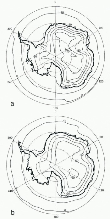
Fig. 1. Simulated (a) annual surface temperature and (b) 2 m air temperature for Antarctica. The contour interval is 5°C.
includes a predictive cloud scheme based on relative-humidity criteria (Slingo, 1987). The cloud scheme allows four cloud types (three-layer clouds and convective clouds). Precipitation results from both moist convection and from super-saturation due to large-scale ascent. A parameterization of the effect of atmospheric gravity waves generated by sub-grid scale orography is also included (Palmer and others, 1986). If the surface temperature is below the freezing point, the precipitation is assumed to be snow; otherwise it is taken as rain.
The land-surface temperature and moisture content are calculated using a three-layer diffusive model. The thermal characteristics of the soil are uniform and constant. They do not lake into account the presence of .snow or ice. A no-flux boundary condition at the bottom of the soil model (approximately 3.4 m thick) is used. This is essential for paleoclimate simulation, because it allows the surface temperature to respond fully to the forcing rather than being lied to some current climatology on long time-scales.
In the moisture budget, snow cover is computed as the balance of snowfall, snow melting and sublimation. In the surface-heat budget, the presence of snow or ice is neglected, except for the solar-flux evaluation. Snow cover and the atmosphere then interact mainly through the albedo. On the land, the albedo varies between the snow-free albedo (fixed to the climatology) and the deep-snow albedo (fixed to 0.8) according to the thickness of the snow cover. Snowmelt occurs when the surface-energy balance demands surface temperatures above freezing point. Surface temperatures are then reset to the freezing point and the excess energy is used to melt the snow.
Most of the diagnostic maps presented here are from a 10 year average present-day simulation. However, in some cases, an additional 1 year simulation has been performed to obtain some diagnostics that were lacking in the previous one. This has minor consequences for the Antarctic ice sheet as the diagnostics do not show a high variability from year to year.
2. Model performance of the antarctic climate
Good model resolution is particularly important for regional climate studies and even more in topography-affected regions as is the case for Antarctica and Greenland. For the internal regions of Antarctica, the spectral envelope topography used with the T42 version of the model is fairly realistic. However, around the edge of the ice sheet, whose slope can be large, this resolution does not correctly represent the rapid variations of surface elevation. Most of the model’s marginal points are at relatively high altitudes. None of the Antarctic ice shelves are considered to be land. The Antarctic continent of the UGCM is represented by 735 points and covers 12.2 × 10⁶ km2, considerably less than the currently estimated true area of 13.9 × 10⁶ km2.
2.1. The surface temperature
The modelled surface (soil upper layer) temperature field of Antarctica (Fig. 1a) is clearly dominated by the topography. Although there seems to be a systematic cold bias (the area average annual mean temperature of Antarctica is −44.7°C), the general pattern agrees quite well with the 10 m borehole climatology of Radok and others (1987). As stressed previously, the high altitude of the marginal areas is responsible for a 5°C deficit along the coast. Comparison with station data shows that the annual cycle of temperature is fairly well simulated at the South Pole (Fig. 2) and inside the northern and eastern coasts, Most of the differences between surface-temperature data and simulation occur on the highest part of the East Antarctic Plateau where the minimum of the simulated annual mean surface temperature is too cold by roughly 15°C. The cold bias seems to be more evident in winter, the coreless winter part of the annual cycle starting later than in the station observations.
Surprisingly, the annual mean air-surface temperature (taken 2 m above the surface) does not show the same cold bias (Fig. 1b). Following Paterson (1994), in dry-snow areas of Antarctica, the mean annual air temperature and
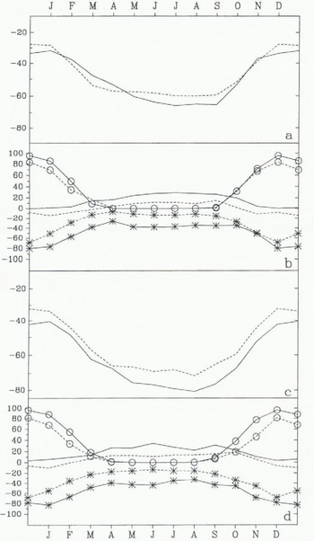
Fig. 2. Seasonal cycle of simulated (full line) and observed (dashed line) (a) surface temperature and (b) surface heat-balance components at South Pole (90° S, 0° E; 2800 m) and (c) surface temperature and (d) surface heat-balance components at Plateau Station (79.3° S, 40.5° E; 3625 m). The heat-balance components are the net shortwave flux (°), the net longwave flux (*)and the sum of the latent- and sensible-heat fluxes. Data from Dutton and others (1989) (South Pole) and from Kuhn and others (1977) (Plateau), the latent-heat and sensible-heat fluxes deduced from the annual cycle.
the 10 m temperature (called firn temperature) should be within 2°C of each other, the firn temperature tending generally to be colder than the air temperature. In the UGCM, the difference reaches up to 20°C on the highest parts of the Antarctic Plateau, the firn being colder than the air.
2.2. The surface heat balance
The heat balance of the surface is the sum of the shortwave, longwave, sensible-heat, latent-heat fluxes and conduction of heat through the surface (all fluxes are defined positive towards the surface and expressed in Wm−2). As this version of the UGCM uses a no-flux boundary condition at the bottom of the soil layers, the heat budget should be zero at each grid point (in a multi-annual average) and at least in an annual a really average over Antarctica. This is effectively almost the case, the residual 0.12 W m−2 is probably due to the fact that the diagnostics are obtained from a single year additional simulation. The surface heat budget shows a balance between the energy gain through the shortwave (32.89 W m−2) and sensible-heat fluxes (19.03 W m−2) and the energy loss through the net longwave surface flux (−51.03 W m−2), The latent-heat flux (0.75W m−2) is negligible compared to the other three. Locally, simulated heat balance has then been compared with the radiative climatologies for Mizuho, South Pole and Plateau Stations (Fig. 2) (all having the advantage of being roughly at the same altitude in the model and reality). Although the annual temperature cycle is quite well simulated at the first two stations, all the points considered show the same trends, enhanced at the Plateau grid point. The simulated surface shortwave flux is generally slightly overestimated. This could be due to a lower albedo or to a sparser cloud cover. The maximum value of 0.8 for the snow albedo is effectively too low. As pointed out by Schwerdtfeger (1984), the mean albedo for Plateau station between October and February is 0.84. The surface loss of energy, through the longwave flux is clearly overestimated. As the surface temperature is already too low, this is probably due to a weakness in the simulated downward longwave flux. This could be related to a lack of cloudiness, or to an incorrect radiative effect of the clouds. The model seems to overestimate the cloudiness, so the explanation can probably be found in some misrepresentation of the optical cloud properties. The simulated sensible-heat fluxes are generally too high, which firs well with the observed cold bias.
2.3. Cloudiness
The annual area-averaged cloudiness simulated by the UGCM is equal to 72% but it shows a fairly large spatial variability (22–100%) with a standard deviation of 15%. The highest cloud cover occurs on the Antarctic Plateau, in some places along the coast and on the Antarctic Peninsula. Cloudiness is more important in winter, the area-averaged June cloudiness equals 85%, while the December value falls to 60%. Comparison with the sparse data stations (Fig. 3) seems to indicate that the simulated winter cloudiness of the Antarctic Plateau is too high. This is in apparent contradiction with the weakness of the downward surface longwave flux. But often, saturation and oversaturation happens over the highest parts of the ice sheet and does not form clouds as a result of the low absolute amount of water vapour present at these altitudes (Bromwich, 1988). This is the cause of frequent clear-sky ice-prism precipitations during the colder seasons (Kuhn, 1970). As the model was originally developed for middle and low latitudes, air saturation is always associated with cloudiness. An appropriate algorithm, taking into account the absolute amount of water vapour and the infrared radiative properties of the ice crystals, could improve the simulated cloud cover and downward infrared flux.
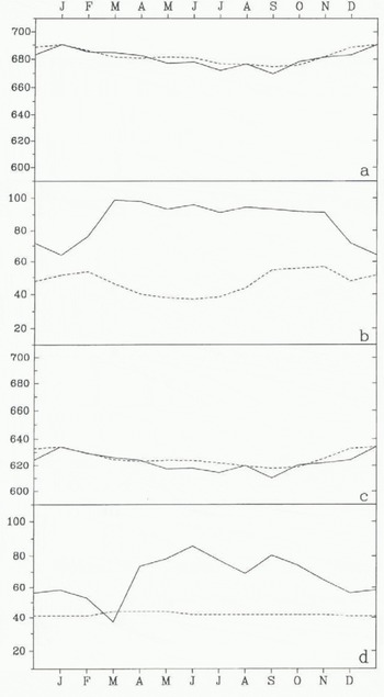
Fig. 3. Seasonal cycle of simulated (full line) and observed (dashed line) (a) surface pressure and (b) cloudiness at South Pole (90° S, 0° E; 2800 m) and (c) surface pressure and (d) cloudiness at Vestok Station (78.45° S, 106.87° E; 3420 m). Data from Jones and Limbert (1987) for the surface pressure and from Warren and others (1986) for the cloudiness.
2.4. Precipitation and accumulation
The UGCM estimates the mass balance of Antarctica (snow precipitation minus snow melting and evaporation–sublimation) to be 1686 × 10−12 kg year−1, which represents an area-average of 138 mm year−1. Although this value is at the lower bound, it falls within the range of accumulation values (from 125 to 210 mm year−1. compiled by Giovinetto and Bull (1987), most of these values are excluding the Antarctic Peninsula. From their accumulation map based on field observations, Giovinetto and Bentley (1985) calculated an area-averaged (excluding the Antarctic Peninsula) accumulation rate of 143 ± 14 mm year−1 (corresponding to 1468 × 1012 kg year−1). Fortuin and Oerlemans (1990) found, using an independent data set, a mass gain at the surface of 1817 × 1012’ kg year−1 (177 mm year−1). Masuda (1990), from the moisture transport deduced from the 1979
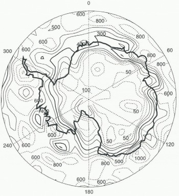
Fig. 4. Simulated snowfall over Antarctica (mm of water eq. Year−1), Contours are 50, 100 (both represented by dashed lines), 150, 200, 300, 400, 500 (all of them represented by full lines, the 300 contour slightly thicker), 600, 800, 1000 and 1200 (all of them represented by dashed lines) mm of water equivalent year−1.
atmospheric analyses by the European Centre for Medium-Range Weather Forecasts (ECMWF), evaluated that the net mass balance for Antarctica was 136 mm year−1 in 1979. The simulated mass balance is also in very good agreement with the Meteorological Office Unified Model (182 mm year−1; Connolley and Cattle, 1994) and with the ECMWF high-resolution model (1594 × 1012 kg year−1) (Genthon and Braun, 1995). The area distribution of snow precipitation (Fig. 4) agrees quite well with the balance map presented by Giovinetto and Bentley (1985). The most notable features are present in our simulation; the desert accumulation area covers most of the East Antarctic Plateau, a bell of high accumulation rates surrounds the coast of East Antarctica, very high accumulation rates are simulated on the Antarctic Peninsula, the two ice shelves are included in the very arid zone and a band of relatively high accumulation rates (15–25 cm year−1) which runs along the Trans-Antarctic Mountains, separating the western and eastern parts of Antarctica, is well simulated. Some features are less well captured by the UGCM, such as the higher accumulation rates on the southern part of the West Antarctic Plateau.
Summer melting is simulated at a few low-altitude grid points (14 points) along the coast and along the Antarctic Peninsula and represents 50 × 10−12 kg year−1, or an area-averaged melting rate of 4 mm year−1. Although this corresponds to the mean of surface ice-melting data compiled by Paterson (1994), this is not really representative because the altitude plays a major role and the steep margins of Antarctica are poorly represented by the spectral envelope. Total snow sublimation reaches an average value of 8.5 mm year−1. As observed in UNESCO (1978), the highest sublimation rates are simulated along the coast, decreasing to zero inland and reversing to net deposition farther in the center of the ice sheet.
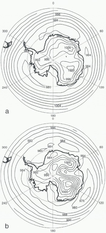
Fig. 5. Simulated sea-level pressure in the southern high latitudes. The contour internal is 4 hPa. (a) Summer (DJF), (b) Winter (JJA).
2.5. The surface pressure
Comparison of the local surface pressure for South Pole and Vostok (Fig. 3) shows very good agreement between observation and simulation in the summer. The winter surface pressure is slightly too low mainly at Vostok but the general agreement is very good.
It is relatively difficult to compare sea-level pressure distributions over the Antarctic continent, because of the elevated topography and the different pressure-reduction algorithms that can be used. Over the peripheral seas, during the summer months (December, January, February) the observed sea-level pressure consists of a circum-polar belt of low-pressure centres located near the Bellingshausen and Ross Seas and in the Indian and South Atlantic Oceans. The lows are about 10–15° of latitude wide with a central pressure around 984–988 hPa. In winter, the strength of the lows increases, The UGCM represents quite well the sea-level pressure field and, in particular, the deep Antarctic trough and the longitudinal position of the lows in summer (Fig. 5). However, the pressure seems to be too deep by roughly 4 hPa and the minimum of the zonal mean sea-level pressure is situated too far south. In winter, there is effectively a deepening of the low situated in the Indian Ocean, while the others become weaker.
2.6. Wind pattern
The wind regime of Antarctica, which is under the influence of large-scale circulation and the katabatic regimes, shows a great directional constancy (Schwerdtfeger, 1984). The katabatic winds are generated by the strong radiative cooling that occur on the Antarctic Plateau and which force air to flow from the interior towards the sea along the slope of the ice sheet. Friction forces, large-scale pressure gradients and the Coriolis force account for the observed wind direction relative to the local ice slope (James, 1989, 1993). During the katabatic events (which can last for several days) convergence of the winds in the icy valleys can result in very high local wind speeds (often more than 50 m s−1; Pettré and André, 1991). These very intense winds are responsible for the break-up and dispersion of the sea ice around the Antarctic ice sheet, and are a prime component of the climate of the polar and sub-polar regions (Bromwich and Kurtz, 1984).
As the model does not resolve the small features of the topography, the simulated wind velocities cannot reach the extreme values cited previously but must be compared to mean wind speeds that are generally observed along the coast (about tens of m s−2; Schwerdtfeger, 1984). The model performs well in simulating the average wind pattern (Fig. 6) when compared to the reconstruction of Mather and Miller (1967) and the simulation of Parish and Bromwich (1991). The wind speeds are also well simulated. Annual mean wind speeds on the Antarctic east coast are of the order of 15 m s−1. They are slightly less on the west coast (± 8 m s−1). Highest speeds are simulated during the sunless months, as observed. The mean June, July and August wind speed reaches 20 m s−1 on the eastern coast.
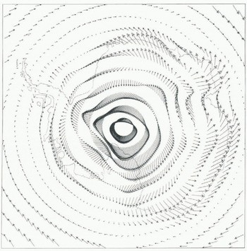
Fig. 6. Simulated wind pattern of Antarctica (m s−1). The longest arrow represents a 20 m s−1 wind.
3. Conclusions
Although the snow-related parameterizations of the UGCM are relatively crude, the simulated Antarctic climate is in good agreement with the available observations and the precipitation/accumulation pattern appears fairly reasonable. The simulated pressures above and around Antarctica are in good agreement with the observations and the general circulation pattern seems to be correctly represented. The low-level winds on the continent are well simulated, given the resolution of the model. The biggest imperfections appear to be related to the surface temperature and the energy budget. The snow-albedo parameterization has to be refined and, as we stressed before, the cloud scheme used in the UGCM could not be adapted to these very extreme conditions, As the Antarctic ice sheet experiences no inching, the animal cycle of surface temperature has no influence on the snow budget, but it could become an important factor in studying past or future climates.
In the future, the ice shelves should he included in the soil domain and the land/sea mask adapted to represent correctly the Antarctic area, faking into account the thermal properties of the snow and ice in the soil atmosphere heat exchange could lead to a better understanding of the Antarctic climate. Further investigations should also be conducted following UGCM performance in simulating the Greenland climate, which is more sensitive to the melting–refreezing processes.
Acknowledgements
This research has benefited from an E.C. Human Capital and Mobility Fellowship (EV5V-CT94-5221). J. King, W. Connoley and C. Genthon helped in collecting the data. Their assistance is gratefully acknowledged. I should also like to thank P. Valdes, J.-L. Ricard and M. Blackburn for helpful discussions.


