Introduction

This paper explores how the spatial pattern of mass balance on a glacier or ice sheet affects its steady-state geometry. Qualitatively, the sensitivity of the surface-elevation profile to the mass balance is low because of the high sensitivity of ice flow to thickness and slope (Reference PatersonPaterson, 1994). Thus, differences in ice transport tend to be accomplished largely by velocity variations driven by relatively small geometry changes. From another perspective, the diffusive effect of ice flow smoothes out spatial irregularities. These notions indicate that spatial variations in mass balance would have only a minor effect on the steady-state elevation profile of the surface of a glacier. The principal purpose of this paper is to test systematically and quantitatively how sensitive (or insensitive) steady-state profile shapes are to the details of the spatial pattern of mass balance.

The Question is significant for several reasons. It is common to report measurements of the mass balance of a glacier in terms of one variable (the mean over the glacier area or the total on that area). Observations indicate that year-to-year changes in mass balance can be uniform over the area of some glaciers. On the other hand, there are examples where inter-annual changes in mass balance do depend on position. Energy-balance modeling of mass balance predicts that the gradient of mass balance with altitude could be expected to change substantially with a change in climate regime (Reference Oerlemans and HoogendoornOerlemans and Hoogendoorn, 1989). Therefore, the question arises as to whether the mean balance is sufficient to determine what will happen to a glacier in response to climate change. The effect on glacier volume is of particular interest because that would affect the response time to climate change (Reference Jóhannesaon, Raymond and WaddingtonJóhannesson and others, 1989) and is of hydrological interest because it represents water storage. A related question is what t an be inferred about the mass-balance pattern of a glacier from its geometry ?

We were also motivated by the desire to test time-dependent models to see whether they approached the correct asymptotic steady state. To make such a test we had to have an independent estimate of the final steady state.

In order to quantify the effects from spatial variations in mass balance, we examined the steady-State geometry predicted by a simple glacier-flow model for a sequence of progressively more complex mass-balance patterns.

Model Description

The flow is assumed to be two-dimensional (2-D) in a vertical plane with X horizontal in the direction of flow. The geometry of the glacier is then described by the elevations of the upper surface Z_s(X) and the bed elevation Z_b(X). The thickness is H(X) = Z_s(X) - Z_b(X). It is assumed that the bed Z_b,(X) and the mass balance B(X) are given as functions of X and fixed independent of time. Then H(X) is to be calculated from the flow dynamics and boundary conditions, which will also determine Z_s(X). Because B is specified to depend only on X and not on H, there is no feedback between mass balance and thickness changes. Furthermore, the 2-D aspect of the model means that only effects from along-flow (longitudinal) variations in B are considered, and nothing is learned about effects from across-flow variations in B.

To set the boundaries of the model glacier, it is assumed that the flow starts against a vertical cliff or a fixed-flow divide at X = 0. The balance flux per unit width Q is then defined as

Q(X) increases through the accumulation area, where B > 0, and decreases through the ablation area, where B < 0. The maximum in Q occurs at X_e , which is the location of the equilibrium line. The location of the terminus X _t, is determined by Q(X_t) = 0 with X _t > 0.

Steady state requires that the flux from ice motion is equal to the balance flux at all locations X. Introduction of a dependence of ice flux on thickness and slope leads to

This form for the ice flux follows from vertically integrated ice deformation neglecting surface-parallel stress gradients and basal sliding. It is a commonly used variable in the modeling of glaciers and ice sheets (Reference PatersonPaterson, 1994). In Equation (2), n is the power in the assumed ice-flow law (Glen's Law) and K is a variable depending on gravitational-force density, flow-law parameters, enhancement factor from fabric, and vertically averaged temperature with a weighting that accounts for variation of stress with depth. These calculations assume that ice density, fabric and temperature are independent of X, and K is constant.

Equations (1) and (2) define a first-order differential equation that determines H(X) given B(X) and Z_b(X). This steady-State model is similar to the Vialov model for an ice sheet (Reference PatersonPaterson, 1994), but allows non-uniform B and Z _b.

To facilitate development of numerical solutions, we introduce dimensionless variables {x, zb, z_s, h, b, q} defined as {X/[L], Z_b/[H], Z_s/[H], H/[H], B/[B], Q/([B][L])}. We take [L] to be approximately the glacier length, [H] to be approximately the elevation difference between the surface at the head and the terminus, and [B] to be approximately the mean accumulation rate in the accumulation area. Introduction of these scalings into Equation (2) gives

where . To mitigate the singularity in Equation (3) at x_t where h = 0, we introduce the substitution

which reduces Equation (3) to

Equation (5) was solved for n = 3 subject to the boundary condition that f(x_t) = 0, which is equivalent to h(x_t) = 0. Commercial solution packages with adaptive gridding were used to produce numerical solutions. Accuracy was tested by comparison to known analytical solutions for spatially uniform or stepped-balance distributions (Reference PatersonPaterson, 1994) and by checking the sensitivity of the results to error tolerances in the solution packages.

Spatial Response

We are concerned with the change in thickness h caused by a change in balance b. Therefore, we set up a reference state for a given z _b described by (equivalently as defined by Equation (1)) and . It is understood that the spatial pattern of this reference state could, in principle, be complex. However, we will consider only the reference states described in figures 1 and 2. These are denoted by a:1, a:2, b:1, .,., d:2, where the number refers to the balance pattern (Fig. 1) and the letter to the bed geometry (Fig. 2). We then examine the steady-state deviations in h from a given reference state forced by a change in b. The deviations are represented as and . We examine different with varying degrees of spatial complexity and determine what characteristics of they cause. The actual calculations are done by solving Equations (4) and (5) numerically with b and h, so it is not necessary for the deviations and to be small compared to the reference values and .

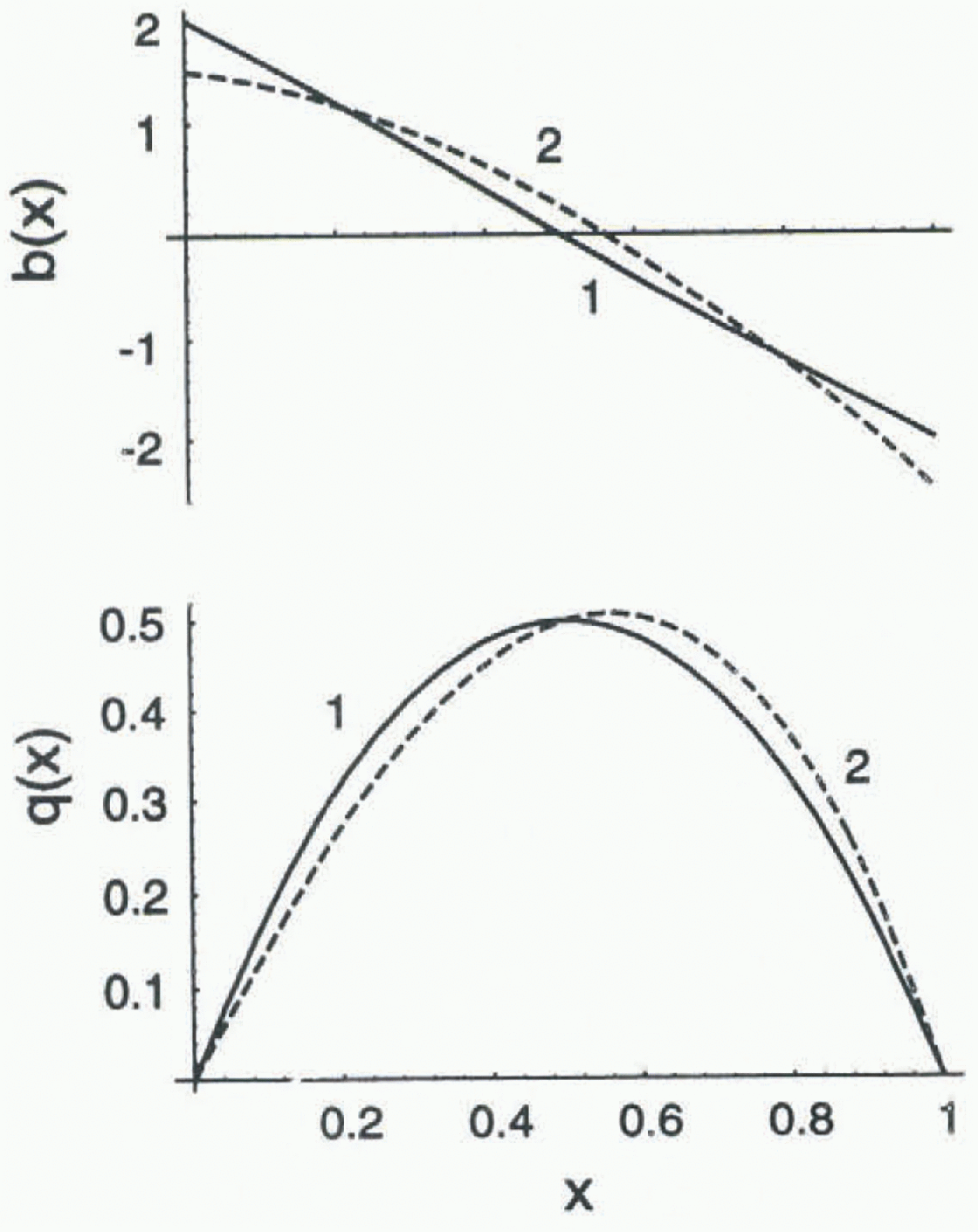
Fig. 1. Example distributions of reference balance (x) (labeled 1 and 2).

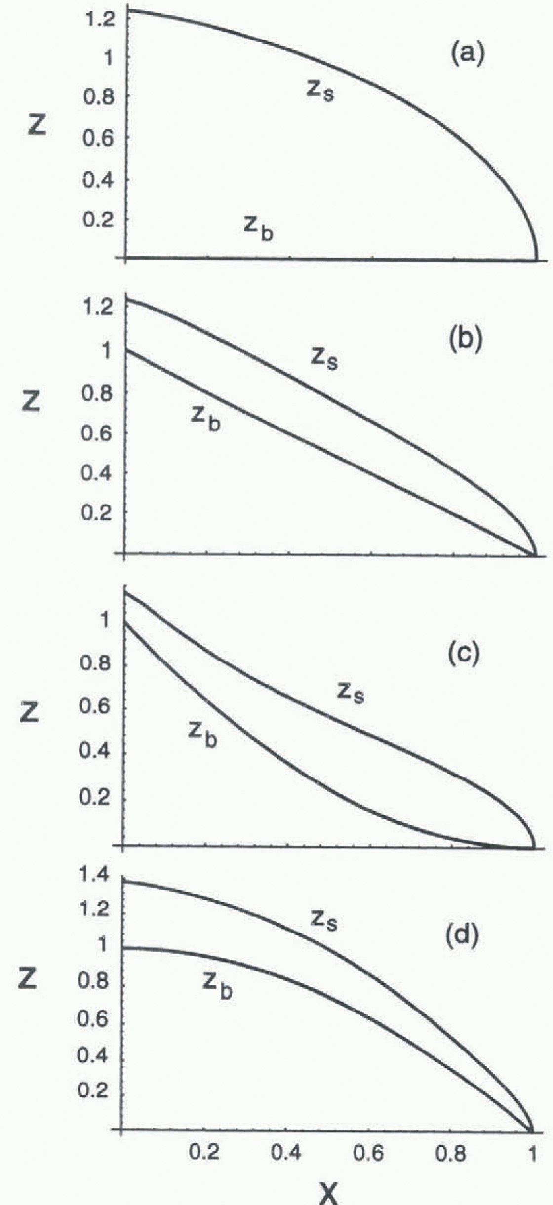
Fig. 2. Model results for reference surface profiles z_s(x) resulting from several combinations of reference bed geometry z_b(x) (labeled a, b, c and d) and b(x) (1 and 2 in Fig. 1). The different surfaces Z_s(x) for a given bed z_b(x) associated with the balance distributions 1 and 2 are not distinguishable at the plotting scale.

We choose [L] = X_t as defined by the reference balance , so that the dimensionless reference length is 1.

Legendre polynomials P_j(x) are used to represent the spatial characteristics of both and over the reference length [0, 1]. The P_j(x) are normally defined on [−1, 1] as

with P ₀ = 1 and P₁ = X. For our purpose, the P_j(x) are shifted and compressed to [0, 1] by defining

Figure 3 shows that increasing orders of P_j(x) represent increasingly fine spatial structure. The P_j(x) form a complete orthogonal set on [0, 1] with the property

Figure 3 illustrates several other important properties of the p_j(x): p_o(x) = 1; the average over [0,1] denoted by is 0 for j > 0 ;p_j (1) = 1 for j ≥ 0.

Fig. 3. Spatial pattern of the scaled Legendre polynomials P_j(x) defined by Equations (6) and (7) for order 0 to 3.

For a given reference state , we consider distributions of b(x) that are represented by βpj(x) one order at a time for j = 0,1, 2,.,.; p_j(x) represents the spatial pattern and β gives the amplitude. Since p_j (1) = 1, there is a decrease in the ablation rate at the terminus (x = 1), when β > 0, and β < 0 gives the opposite effect. Furthermore, since for j > 0. derived from p_j(x) with J > 0 do not change the mean balance (0) over the reference length, and therefore do not cause a change in length. More directly in terms of balance: +p₀(x) is a spatially uniform shift causing an increase in the mean balance on the reference length: +p₁(x) decreases the balance gradient; +p₂(x) decreases the down-glacier increase in balance gradient, which we refer to here as balance curvature.

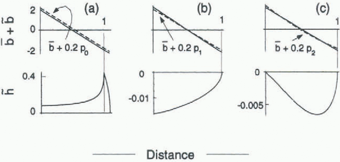
Figure 4 shows examples of calculated for equal to 0.2p₀(x), 0.2p₁(x) and 0.2p₂(x) applied to the reference state a:1 (Figs 1 and 2). Notice that all three of the changes in mass balance correspond to a reduction of ablation at the terminus by 10%. The deviations are largest for , which has a non-zero mean (0.2). This balance deviation causes an increase in length of 10% and an increase in volume of 18%. Even though the balance deviations 0.2p₁(x)) and 0.2p₂(x) have zero means and do not alter the length, they both cause a reduction in glacier volume. The balance deviations 0.2p₀(x) and 0.2p₁(x) result in a reduction in surface slope, and all cause a decrease in the upward convexity of the surface profile over most of the glacier length.

Fig. 4. Thickness deviations produced by balance deviations for the reference state a:1 (Figs 1 and 2) (linear variation of and flat bed Z_b = 0). In the upper panels, solid lines represent reference balance and dashed curves represent disturbed balance + .

We describe the that results from as

The quantity represents the topographic response to a p^j deviation in b of size β projected onto p_i , and is given by

By reference to Figure 3 and Equation (10), for can be interpreted in terms of geometrical changes induced by as follows: gives die increase in volume, is a measure of the decrease in slope and is related to the decrease in upward convexity of the surface.

Figure 5 shows how depend on β for the reference state a:1 (Figs 1 and 2). For β > 0, Figure 5 shows the features concerning change in volume, slope and convexity earlier illustrated in Figure 4 for β = 0.2. The opposite effects are predicted for β < 0 when ∣β∣ is small. For ∣β∣ ≤ 0.1, are approximately linear in β. For larger β, the linearity can break down, as is apparent in Figure 5. Of course, this is expected, because Equation (3) is non-linear. (In this regard, it is important to recognize that in general can not be represented as the superposition of the effects from indiv idual p_j(x) components of an arbitrary mass-balance change. Such a superposition would be valid only in the ease that β_j are small enough to remain in the linear range for all j.)

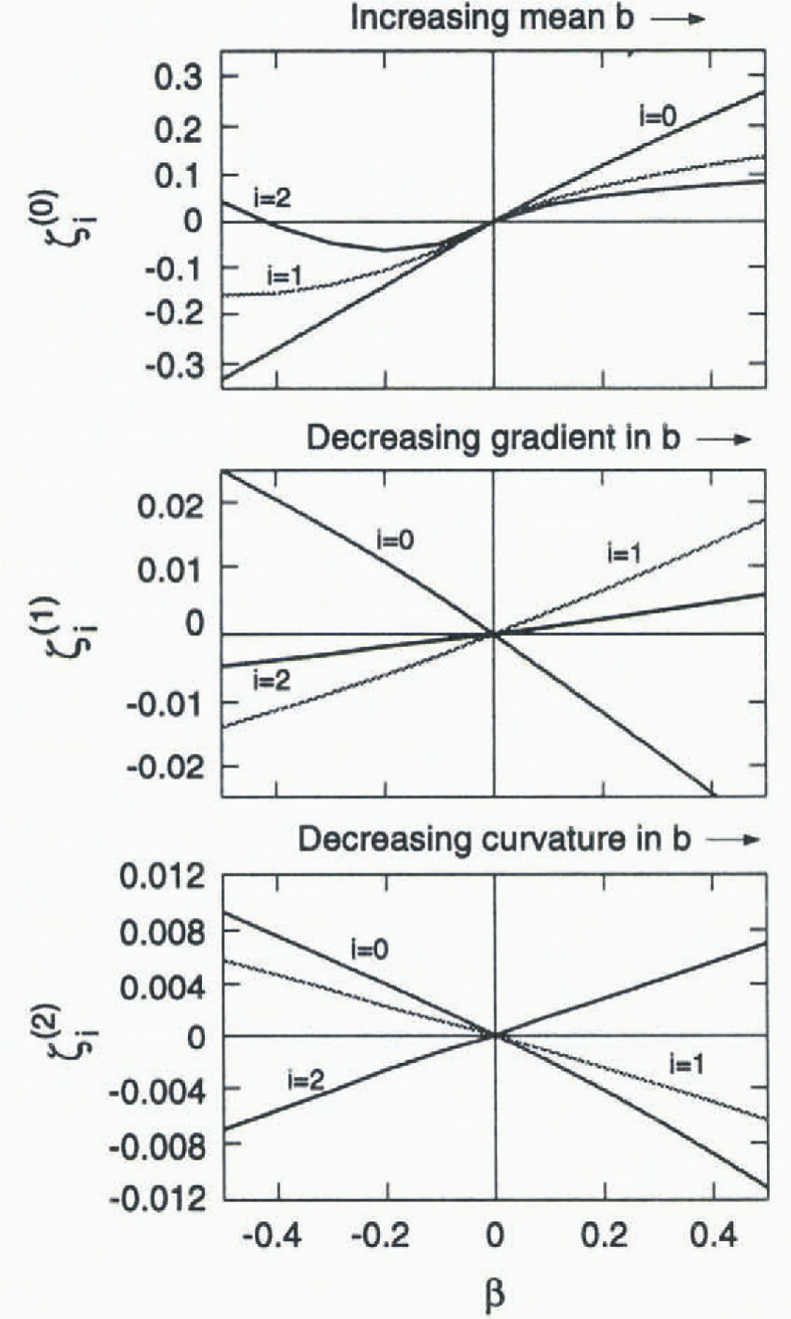
Fig. 5. Topographic response coefficients defined in Equations (9) and (10) calculated for balance deviations corresponding to changes in balance mean (j = 0, top panel), gradient (j = 1, center panel) and curvature (j = 2. bottom panel). Solid curves show topographic response coefficients (Equation (10)) for volume increase , slope decrease (i = 1) and convexity decrease (i = 2). The results shown are for reference state a: 1 (Figs 1 and 2) (linear variation of and flat bed z-b = 0).

The sensitivity of volume, slope and convexity to different spatial patterns of can be represented for small β through sensitivity parameters defined as

where

represents the projection on p_i(x). These parameters are the slopes of the curves in Figure 5 at β = 0, scaled to give the fractional change in geometry characteristics of the surface profile (e.g. volume i = 0, slope i = 1 or convexity i = 2) caused by a unit fractional change in terminus balance for the different spatial patterns of balance change (e.g. mean j = 0, gradient j = 1 or curvature j = 2). For example, S ₀ ⁽¹⁾ gives the fractional changes in volume caused by unit fractional change in balance at the terminus associated with a change in balance gradient. The results for reference stale a:1 (Figs 1 and 2) are shown in Figure 6.

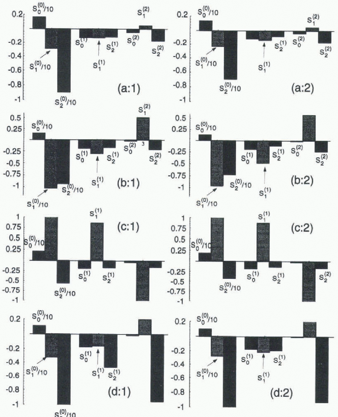
Fig. 6. Shape sensitivity parameters s_i ^(j) defined in Equation (10), (11) and (12). Columns show results for different reference balance (Fig. 1). Rows show results for different reference bed (Fig. 2). Note that sensitivity to shifts in the mean balance shown as s_i ⁽⁰⁾ are divided by 10 for display in this figure.

The same process was followed for the other reference states by imposing a similar selection of on them. The corresponding sensitivity diagrams are also shown in Figure 6. All of these examples show the same systematics with regard to effects on volume, slope and convexity of the thickness profile. The apparently reversed slope effects for the concave bed (geometry c) arises because the reference state is thickess in the lowest part of the profile and the thickness gradient is opposite to the other examples, which are thickest in their upper reaches (Fig. 2).

Discussion

The main result shown in Figure 6 is that the effects on volume, slope and convexity are one order of magnitude larger for a spatially uniform variation in b compared to a change in b that has non-zero mean with the same change at the terminus. A uniform change in b causes changes in thickness that are concentrated in the lower part of the glacier profile, which results in large changes in slope and convexity of the surface (Fig. 4). Clhanges in b with zero mean cause changes in thickness that are largest in the mid- to upper-parts of the glacier profile (Fig. 4). The effect on volume has the opposite sense when comparing zero and non-zero mean changes that have the same change in b at the terminus.

The details of shape sensitivities do not depend significantly on the reference mass-balance pattern (compare columns 1 and 2 in Fig. 6), but there is considerable dependence on the bed geometry (compare rows a, b, c and d in Fig. 6). An important example is that the fractional change in volume per unit change in mean balance in units of terminus ablation rate varies from about 1 to 2 (S₀ ⁽⁰⁾ in Fig. 6). The larger numbers are associated with low bed slope (geometry a) especially near the terminus (geometry c).

It has long been recognized that the change in steady-state length of a glacier is related to the change in mean mass balance by continuity without regard to Iflow dynamics (Reference NyeNye, 1960). The time-scale to complete the change in length is controlled primarily by the volume change required to reach the new steady state : (Reference Jóhannesaon, Raymond and WaddingtonJóhannesson and others, 1989). This time-scale describes how long a glacier “remembers” prior climate. Evidently, it is very insensitive to the spatial pattern of mass balance that causes the changes.

It is of interest to ask whether information about the spatial pattern of the mass-balance change might be found in the changes in glacier geometry up-glacier from the terminus. The results of these calculations indicate that while the glacier shape is affected by the spatial pattern of mass balance, the effects are very small and are likely to be obscured by factors in nature that are not accessible to precise analysis (for example, details of the bed geometry, the physical controls of flow or transient response to climate change). In this regard, it is important to recognize that the conclusions of these calculations can not be extended to short-length scales, where longitudinal coupling Reference Kamb and EchelmeyerKamb and Echelmeyer, 1986) suppresses diffusion effects that smooth the profile (Reference Langdon and RaymondLangdon and Raymond, 1978). It is also important to keep in mind that these calculations specify balance as a function of position, and the feedback between mass balance and geometry can be different than when balance is specified as a function of altitude and the slope of the bed is low.

The most important potential change in b with a zero mean is a change in balance gradient, which would have similarity to a deviation of die Iinni βp₁(x). For example, in main eases a likely effect of climate warming is an increase in balance gradient (Reference Oerlemans and HoogendoornOerlemans and Hoogendoorn, 1989), which corresponds to β < 0 and predicts a consequent increase in volume. The volume increase is necessary to allow a larger flux q in the central part of the profile. The volume sensitivity to a change in balance gradient is about 0.1-0.2 (s ₀ ⁽¹⁾ in Fig. 6), which is much smaller than the volume sensitivity to change in mean mass balance of about 1-2 (s ₀ ⁽⁰⁾ in Fig. 6).

In reality a change in balance gradient may be larger in the ablation area than the accumulation area (Reference Oerlemans and HoogendoornOerlemans and Hoogendoorn, 1989). This would have an added effect of increasing the curvature of the spatial pattern of mass balance described like βp₂{x) with β < 0. The consequence would still be to increase the volume slightly, but at a sensitivity that is yet smaller : s ₀ ⁽²⁾ in Fig. 6).

Conclusions

'Fhe principal conclusion is that most of the information relevant to the geometry of a glacier is contained in the mean mass balance. Details of the spatial pattern of mass balance affect the geometry, but the effects are more than one order of magnitude smaller than those driven by the mean.