Introduction

Antarctic sea ice is greatly influenced by the dynamic nature of the Southern Ocean. Ocean waves can propagate from tens to hundreds of kilometres into sea ice (Reference Kohout, Williams, Dean, Meylan, Komen, Cavaleri, Donelan, Hasselmann and HasselmannKohout and others, 2014), leaving behind a wake of broken ice floes. Over recent decades, the frequency of storms has increased in the Southern Ocean (Reference HartmannHartmann and others, 2013), and wave heights are predicted to increase in the future (Reference Dobrynin, Murawsky and YangDobrynin and others, 2012). Increased storm intensity will bring stronger winds and larger, longer waves, with the potential to travel deeper into the ice pack, increasing the likelihood that ice floes break apart.

Understanding the complicated physical processes of waves-in-ice theory has been a topic of interest for several decades (e.g. Reference Squire, Dugan and WadhamsSquire and others, 1995; Reference SquireSquire, 2007), and has evolved to a point where a more accurate representation of wave decay in sea ice could be included in wave models (Reference SquireSquire and others, 2009; Reference WangWang and Shen, 2010, Reference Wang2011; Reference Dumont, Kohout and BertinoDumont and others, 2011; Reference Bennetts and SquireBennetts and Squire, 2012). The theory, however, has typically depended on measurements collected in the Arctic during the 1970s and early 1980s (e.g. Reference Wadhams, Squire and GoodmanWadhams and others, 1988), from experiments conducted over short timescales and in relatively low-amplitude ocean swells. Additional experiments have since been conducted in the Antarctic (Reference Hayes and JenkinsHayes and Jenkins, 2007; Reference Doble and BidlotDoble and Bidlot, 2013), but a more comprehensive dataset is still required.

To work towards this, we designed a series of waves-in-ice observation systems (WIIOS) to measure waves in Antarctic sea ice. These were deployed on East Antarctic sea ice from RV Aurora Australis, during the Australian-led second Sea Ice Physics and Ecosystem Experiment (SIPEX II). The purpose of SIPEX II was to investigate relationships between the physical sea-ice environment, marine biogeochemistry and the structure of Southern Ocean ecosystems. Upon entering the pack-ice zone, five WIIOS were deployed on the sea ice along a meridional transect line. Every 3 hours, the WIIOS simultaneously woke and recorded wave accelerations for 34min. On 23 September 2012, three WIIOS were deployed via a helicopter hovering ∼2 m above the floe. The remaining WIIOS were deployed via RV Aurora Australis’s aft 7t crane. This was achieved in high winds (up to 2 5 ms^–1 ) and 2-3 m swell. Each WIIOS performed on-board data quality control and spectral analysis before returning the wave spectrum via satellite.

Our aim was to capture the attenuation of wave energy as it propagates into sea ice. There are, however, various levels of complexity associated with extracting wave attenuation. To accurately describe the attenuation, one must consider wave direction, ice conditions, ice extent, storm duration and wave speed. Due to the logistical challenges of the study site, complications due to the proximity of magnetic south, and the duration of the experiment, these details were not comprehensively measured. Reference Kohout, Williams, Dean, Meylan, Komen, Cavaleri, Donelan, Hasselmann and HasselmannKohout and others (2014) analyse this dataset, managing these complexities by applying assumptions and using approximations from satellite imagery. Any errors are minimized by focusing on the significant wave heights, the median decay rates and excluding outliers.

In this paper we summarize the dataset, excluding the assumptions used by Reference Kohout and WilliamsKohout and others (2014). We also describe, in detail, the hardware and software design of the WIIOS. The raw data and metadata are available via Reference Kohout and WilliamsKohout and Williams (2013). All dates throughout this paper are referenced to coordinated universal term (UTC).

Hardware Design

The WIIOS consisted of a single printed circuit board with two processors and four daughter boards. The main sensor was a high-resolution Kistler ServoK-Beam accelerometer (model 8330B3). The Kistler is an analog force feedback sensor incorporating a silicon micro-machined variable capacitance sensing element that provides excellent bandwidth, dynamic range, stability and robustness. Capacitive accelerometers are less prone to noise and variation with temperature, typically dissipate less power and can have larger bandwidths. The Kistler has a range of ±3g (1g = 9.80665 ms^–2 ), a sensitivity of 1200 m V g ^–1, a resolution of 1.3 μg and a –40°C operating temperature limit. Each WIIOS also included a GPS, an Iridium transceiver and lithium batteries. A lower-resolution 9 degrees-of-freedom Razor inertial measurement unit (IMU) was also included in the package. This IMU incorporates an ITG-3200 micro-electromechanical system (MEMS) triple-axis gyro, an ADXL345 triple-axis accelerometer with 286 mVg ¹ sensitivity and a resolution of 4 mg LSB ¹ (LSB is least significant bits) and a HMC5883L triple-axis magnetometer. The board came programmed with the 8 MHz Arduino bootloader and firmware. The intended use of the IMU was for true vertical acceleration correction and wave direction. Unfortunately, due to magnetic south distortion at the time of the experiment, the calculated wave directions are unreliable. The electronics were sealed in a silicon membrane to avoid condensation and were housed in a watertight container. The container was packed with enough lithium batteries to survive for a minimum of 6 weeks. Finally, the container was fitted inside a tyre for protection and flotation (Fig. 1 and 2). The Iridium and GPS aerials were housed in a plastic spherical container on top of a 0.5 m tube attached to the tyre. Protruding screws were fixed to the underside of the tyre to provide friction with the ice.

Fig. 1. The custom-made circuit board, lithium batteries and the watertight case.

Fig. 2. One of the WIIOS shortly after deployment.

Software Design

Signal conditioning

Prior to carrying out any analysis, the raw acceleration data were conditioned. Following Reference EarleEarle (1996), we ran several basic statistical tests on the raw time series. The number of occasions that consecutive unresponsive (or showing no variation) samples occurred was recorded and the fraction of unresponsive samples in the Kistler record was returned. If >15% of the Kistler data were unresponsive, the flat-lined samples were filled with the IMU acceleration. If >50% of the Kistler, IMU or gyro data were unresponsive, it was assumed the full time series was corrupt and it was therefore flagged as bad. If 100% of the IMU magnetometer data were unresponsive, then the time series was again flagged as bad.

We also put a 0.5g upper bound on the magnitude of the acceleration. For a Stokes 120° corner flow, the limiting form of a non-breaking wave at the crest, the downward acceleration of a water particle in the crest is 0.5g (Reference Tucker and PittTucker and Pitt, 2001). We also identified unlikely occurrences (spikes) using a statistical test. These are usually set at a probability level, meaning that they will occasionally fail on valid data. A general approach is to remove data points that exceed a specified standard deviation (Reference Emery and ThomsonEmery and Thomson, 1998). A weakness with this approach is that the spike itself is included in the calculation of the standard deviation. This can be corrected using an iterative process, in which the values outside the accepted range are omitted from each subsequent recalculation of the mean and standard deviation, until the remaining data have near-constant statistics with each new iteration. Reference EarleEarle (1996) used such an approach, with the limit being three standard deviations over three iterations. According to Chebyshev’s inequality, for all distributions, at least 97% of the data will be within six standard deviations of the mean. We therefore used the standard deviation threshold limit, but used six standard deviations as the threshold. The number of spikes was returned and each spike was removed and linearly interpolated from the adjoining valid points. The maximum number of consecutive spikes in the dataset was also returned.

Trends in the time series should be removed before analysis. Reference Tucker and PittTucker and Pitt (2001) suggest a simple and effective detrending scheme:

(1)

where is the nth detrended signal, y_n is the raw signal, . At the start of the computation, s ₀ is set to zero, and as the filter runs into the data, it settles down exponentially with a time constant of ∆t=(1 k). We applied this scheme with k= 0.9995. With a sample rate of 8 Hz (the rate at which the algorithm was applied), this is the equivalent of a single-stage resistor-capacitor (RC) electronic high-pass filter with a time-constant of 250 s (100 s is the lowest that should be used). It is important to remove the mean before the detrend algorithm is applied. If this is not done, the series will begin at the mean of the raw series (rather than at zero). Eventually the series will settle to a mean of zero, but it will need to run through hundreds of iterations before settling. The spike algorithm was reapplied after the detrending algorithm to ensure no spikes were missed due to the presence of a trend.

As shown by Reference Bender and GuinassoBender and others (2010), the method of using only the vertical acceleration relative to the platform

(2)

to approximate the true vertical acceleration (relative to the Earth, is only sufficiently accurate when the tilt is <10° from the vertical. If the instruments are deployed with an angle >10° the heave will be overestimated. can be calculated given the roll, pitch and the platform relative acceleration along three axes (Reference Bender and GuinassoBender and others, 2010),

where θ is the pitch and ϕ is the roll. Therefore, using the high-resolution z-axis accelerometer, and the lower-resolution x- and y-axis accelerations, combined with the roll and pitch calculated via the IMU and the direction cosine matrix algorithm (as described by Reference Premerlani and BizardPremerlani and Bizard, 2009), we can calculate the true vertical accelerations. However, due to the low resolution of the IMU, if small accelerations are present, then the true vertical acceleration may be less accurate than using only the Kistler. After rigorous testing, we found it suitable to apply the true vertical correction if the tilt was >50°. Otherwise, using only the higher-resolution Kistler was the better alternative. For the duration of this experiment the tilt only exceeded 10° twice (and was flagged as bad on these occasions) and did not exceed 50°, so the IMU was not used to correct the vertical acceleration.

Low-pass anti-aliasing filter and decimation

As we take a discrete sample of a continuous function which is not bandwidth-limited, all wave signals greater than the Nyquist frequency where A is the time interval between consecutive samples) are aliased or falsely translated to signals less than f_c. To overcome aliasing, it is necessary to enforce a known limit on the sample by analog filtering of the continuous signal and sampling at a rate sufficiently rapid to give at least two points per cycle of the highest frequency present (Reference Press and TeukolskyPress and others, 1992). The analog filter is an RC filter, where at 8 Hz the power is reduced to half (3 dB). Following Reference Tucker and PittTucker and Pitt (2001), we oversampled at 640 Hz and decimated to 2 Hz. Down-sampling from 640 to 2 Hz was achieved through a multistage decimation of 80 followed by 4, to achieve a total decimation of 320. The multistage decimation was applied, as it reduces computational and memory requirements of the filters. Prior to each downsampling stage, a second-order low-pass Butterworth filter was applied to remove all components above the Nyquist frequency. We first applied the Butterworth filter with a cut-off of 1 Hz and sampled at 8 Hz, and then with a cut-off of 0.5 Hz and sampled at 2 Hz. A second-order Butterworth filter was chosen, as it has a flat frequency response, i.e. small ripple. The cost, however, is a slow roll-off around the cut-off frequency. We minimized this by selecting cut-offs well within the Nyquist frequency. Note that the effectiveness of the anti-aliasing filter depends on the ratio of the amplitude of the noise to the amplitude of the waves within the band limit.

Integration

We are primarily interested in wave displacement and therefore needed to integrate the acceleration time series. A consequence of integrating the acceleration is large low-frequency drifts from simple integration acting on low-frequency noise. We therefore needed to apply a high-pass filter to cut out the large low-frequency drifts (Reference Tucker and PittTucker and Pitt, 2001). We achieved this by applying a Fourier-transform filter, which is an efficient alternative to a moving-average filter in the time domain. The time series was first Fourier-transformed, multiplied by frequency response weights, R(f), and then reverse-transformed to give the filtered time history. We chose real numbers as the weights to ensure no phase shift was produced. Applying frequency response weights of 1/!² is equivalent to double integration of acceleration. We applied the high-pass filter by enforcing a low-frequency cut-off. To prevent an abrupt cut-off, which leads to a long and slowly decaying convolution array, we smoothed the cut-off using a half-cosine taper (Reference Tucker and PittTucker and Pitt, 2001)

(3)

where f is frequency, f_c is the Nyquist frequency and f and f2 vary depending on the specific requirements of the task. Since we were taking a finite record from an infinite source, transients were introduced at the two ends of the record. The effects of these transients after filtering can be significant, and can distort the statistics of the wave heights. The solution (as recommended by Reference Tucker and PittTucker and Pitt, 2001) is to design the filter to restrict the effect of these transients to a short time at each end of the record, and abandon the affected parts (Fig. 3). Following Reference Tucker and PittTucker and Pitt (2001), we selected f = 0.02 and f2 = 0.03, which are suitable for a frequency bandwidth of 4-20s and reduce the convolution function to ∼120s.

Fig. 3. (a) The response function. (b) The wave accelerations after integration and filtering (blue) and the abandoned transients (red).

Spectral analysis

From Parseval’s theorem, and since our time series was real, the power spectral density, PSD, can be defined as

(4)

where C(f) is the time series represented in the frequency domain. Due to data leakage, we can only estimate the PSD. This estimate is known as the periodogram estimate, P. We can minimize leakage by multiplying the input time series, c_j, j = 0,..., N 1, by a window function, wj, which changes more gradually from zero to a maximum and back to zero asj ranges from 0 to N. In typical applications, the window functions are non-negative, smooth bell-shaped curves. Reference Tucker and PittTucker and Pitt (2001) recommend applying a partial cosine taper function. Figure 4 shows weighted displacements for various values of the partial cosine taper coefficient, γ. We used γ = 5 in the WIIOS.

Fig. 4. (a) The partial cosine taper window function for 7 = 1 (solid), 5 (dashed) and 10 (dotted). (b-d) Weighted time series with 7 = 1, 5 and 10, respectively.

Another complication with the periodogram estimate is its variance (Reference Press and TeukolskyPress and others, 1992). Regardless of the number of sampled points, the standard deviation will always be 100% of the value. Following Bartlett’s method, the variance can be reduced by partitioning the original sampled data into K segments, each of 2M consecutive sampled points. This, however, comes at a cost of reduced frequency resolution. Each segment is separately Fourier-transformed to produce an independent periodogram estimate. The K periodogram estimates are then averaged at each frequency. This averaging reduces the variance by a factor of K. Welch’s method extends Bartlett’s method by windowing each segment prior to the Fourier transform. As a result, however, the data at the centre of the window function generally have more influence than the data at the edges, which results in a loss of information. To mitigate that loss, the individual datasets are overlapped in the time domain. Overlapping the segments by half their lengths gives the smallest possible variance per data point (Reference Press and TeukolskyPress and others, 1992). The first and second sets of M points are segment 1, the second and third sets of M points are segment 2, and so on up to segment K, which is made of the Kth and K + 1th sets of M points. The total number of sampled points is therefore (K+ 1)M, just over half as many as with non-overlapping segments. The variance is reduced by a factor of ∼9K/11. Figure 5 gives an example of how we reduced the variance in P. In each WIIOS, we used K = 4 and M = 512. With a 2 Hz sample rate, this gave a segment duration of 512 s. Reference Tucker and PittTucker and Pitt (2001) recommend a minimum of 1000s for minimal leakage. In our case, we have ensured minimal leakage by applying a window on each segment.

Fig. 5. An example of how we reduce variance in the periodogram estimate, P. (a) The windowed time series of each segment (K1,K2,K3,K4); (b) the periodogram estimate of each segment; and (c) the average periodogram estimate at each frequency. The shaded regions in (b) and (c) give the standard deviations of the estimate.

Tucker and Pitt (2001) show how averaging the harmonics, once the record has been analysed, is another effective way to reduce leakage. If the Fourier transform is computed using finer frequency resolution than is required, the neighbouring estimates can be averaged together. An odd number of bins is used, to ensure the centre frequency of the bin remains well defined. Each WIIOS reduced the 512 bins to 55 by averaging five bins for periods <6s and >20s and by three bins for periods between 6 and 8s. To maintain resolution, periods between 8 and 20 s were not averaged.

Useful definitions and statistical results can be expressed in terms of the moments of the PSD. The nth spectral moment is defined by Reference Tucker and PittTucker and Pitt (2001) as

(5)

where P is the periodogram estimate of the PSD. The m ₂ to m3 moments were returned, enabling the calculation of the key statistical results. Note that we calculated the spectral moments before frequency averaging. The significant wave height, H_s, is calculated from the zeroth spectral moment, defining the total variance (or energy of the wave system),

(6)

Confidence intervals

Confidence intervals for the power spectra are given by Reference EarleEarle (1996) as

(7)

where x² are percentage points of a chi-square probability distribution and a defines the confidence interval, i.e. α = 0.9 provides a 90% confidence interval. DoF is the degrees of freedom. For cosine windowed overlapping segmented data, the DoF can be approximated by (Reference EarleEarle, 1996)

(8)

A reduction in this interval is obtained by averaging the harmonics. If L bins are averaged together, the variance (and DoF) is reduced by a factor L. The 90% confidence interval for H_s is approximately 10 to +15% (Reference EarleEarle, 1996). A summary of the variables used in each WIIOS is given in Table 1 and a list of the transmitted variables in Table 2.

Table 1. A summary of variables used during analysis

Table 2. Transmitted data

Testing

A number of testing methods were used throughout the construction of the sensors. Each electrical component was tested in a -20°C freezer for failure and endurance. As the Kistler accelerometer is inherently linear, each individual unit was tested at 1g, obtaining specific offset and gain for each completed assembly. The IMU was factory-calibrated. We found the differences between the two sensors were minimal for accelerations within the limits of the IMU. The software and filtering processes were tested via a series of various pure sine waves, sine waves with artificially generated white noise and acceleration time series from the Ross Sea marginal ice zone (Reference DownerDowner and Haskell, 2001). The combined hardware and software was tested using a purpose-built calibration rig, which included a vertical slide driven by a connecting rod to a rotating wheel. To minimize noise, the motor driving the wheel was very low-geared and controlled with pulse-width modulated power. The wheel was driven by a soft elastic belt. The speed and amplitude of the wheel could be varied and we tested amplitudes in the range 0.03-0.20 m, wave periods 5-20s and accelerations 0.03-50mg. For periods >20s and amplitudes <0.032 m, the test rig and component noise were too great to detect the wave source. The platform could also be pivoted to test the roll and pitch. As a final test, the sensors were deployed in a coastal environment to test measurement and analysis of real wave motion.

Results

In total, we collected ∼600 records of wave spectra over 39 days. We captured our first large wave event shortly after deployment, losing our first instrument, which experienced 2 5 m s ¹ winds and at least 6 m significant wave heights. The second large wave event occurred on 1 October 2012. During this event, we lost another two WIIOS, each of which had lasted a total of 9 days. The next large wave event occurred on 9 October 2012, during which we lost the fourth WIIOS, after 17.5 days. Our final instrument stopped transmitting on 2 November 2012 (Fig. 6). The WIIOS were deployed on floes in the Antarctic marginal ice zone, the region where the open ocean meets the sea-ice pack. Upon deployment, the ice region consisted of individual floes between 2 and 100 m wide, brash ice, grease ice, frazil ice and nilas ice (Fig. 2). We deployed on floes with freeboards <1 m thick and <25 m wide (Table 3). The average floe thickness along the deployment transect ranged between ∼0.5 and 1 m and the majority of floe diameters were 2 - 20 m, depending on their distance from the ice edge. The ice concentration for the duration of the experiment was higher than the mean for this region (Reference Kohout, Williams, Dean, Meylan, Komen, Cavaleri, Donelan, Hasselmann and HasselmannKohout and others, 2014).

Fig. 6. An overview of the location and significant wave heights for each WIIOS (green, red, orange, purple, blue) for the duration of the experiment. (a) The distance, X (km), from the ice edge. (b) The significant wave heights, H _s (m).

Table 3. Approximate floe dimensions (freeboard (FB), width and length) of each WIIOS and the latitude, longitude and distance from the ice edge (X) of each WIIOS upon deployment

Quality control of the full dataset is maintained by returning the mean acceleration and orientation, acceleration and rotational velocity standard deviations, general data quality flags, the number of spikes and unresponsive samples and the power difference between domains (Table 2). A small number of data records were rejected (Table 4). The majority of these were due to too much noise in the gyro standard deviations or too many spikes occurring within the record.

Table 4. The number of data points and missing values for each WIIOS

Frequency distributions of the significant wave heights and peak periods for the entire dataset are provided in Figure 7. The majority of data collected closest to the ice edge were obtained during calm periods, with significant wave heights of 1 –2 m. Further into the ice (>100 m from the ice edge), the majority of waves recorded were 0–1 m. The majority of waves near the edge have peak periods ranging between 10 and 12 s, and the peak periods further into the ice were 14–16s. In summary, as expected (Reference Squire, Dugan and WadhamsSquire and others, 1995), the wave height generally decreased and the peak period increased as the waves propagated into the sea ice.

Fig. 7. The distribution of (a) significant wave heights and (b) the peak periods for the full dataset. The blue and red bars represent data when the WIIOS are within and beyond 100 km of the ice edge, respectively.

Figures 8–12 examine the ice concentrations (Reference KaleschkeKaleschke and others, 2001; Reference Kaleschke and KernKaleschke and Kern, 2006; Reference Spreen, Kaleschke and HeygsterSpreen and others, 2008), hindcast approximations for wave direction (Reference Chawla, Spindler and TolmanChawla and others, 2013), locations, wave heights and wave spectra of five different records.

Fig. 8. (a) The location of each WIIOS (markers), ice concentration (%, contours) and hindcast wave directions (arrows) on 27 September 2012 at 02.00. (b) The significant wave heights, H _s, over time (curves) and on 27 September 2012 at 02.00 (markers) of each WIIOS. (c) The power spectral densities, PSD, of each WIIOS on 27 September 2012 at 02.00. The solid, dashed, long dashed and dotted curves correspond to the square, circle, triangle and diamond markers, respectively. The shaded regions in (b) and (c) give the 90% confidence intervals.

In Figure 8, the conditions on 27 September 2012 at 02.00, during small waves, are considered. The WIIOS are roughly aligned perpendicular to the ice edge. The offshore swell direction from the hindcast is likely to be an error in the model and suggests offshore winds were present (Fig. 8a). The decay of the short-period waves and the persistence of the long-period waves in Figure 8c aligns with the commonly accepted theory presented by Reference Squire, Dugan and WadhamsSquire and others (1995). Figure 9 also considers the WIIOS record during small waves, but on this occasion two spectral peaks are measured near the ice edge. Figure 9c shows how these two peaks evolve as the waves propagate into the ice field. The wave hindcast shows variable wind directions and is again unreliable. On this occasion, the WIIOS are again roughly aligned perpendicular to the ice edge.

Fig. 9. Same as Figure 8, but for data from 26 September 2012 at 5.00.

Figure 10 shows the conditions during a large wave event on 23 September 2012at 20.00. On this occasion, the WIIOS are roughly in line with the hindcast wave direction, providing an ideal opportunity to measure wave attenuation. Also, note that the peak significant wave height occurs at 17.00 at each WIIOS, so simultaneous comparisons are possible. The spectra suggest that as the wave propagates through the ice, the energy at the peak wave period cascades toward longer periods, leading to energy growth (rather than decay) at certain periods. This is indicative of nonlinear interactions in a growing wind sea (Komen and others, 1994).

Fig. 10. Same as Figure 8, but for data from 23 September 2012 at 20.00.

Figure 11 shows an example of a more complicated case. First, the northernmost WIIOS (square and circle markers) are parallel to the wind direction, rather than perpendicular (Fig. 11a). Interestingly, the spectra from the two WIIOS (solid green and dashed red) are very different (Fig. 11c). Perhaps this is due to significantly differing distances, as a result of the angle of the incident wave, that the waves have to propagate through ice before reaching each WIIOS. The deeper two WIIOS (triangle and diamond markers) are, however, in line with the wave direction, and their spectra show decay, as would be expected from standard waves-in-ice theory (Reference Squire, Dugan and WadhamsSquire and others, 1995). Also note that the peak of these deeper buoys occurs 3 hours later than the outermost buoys, presumably again due to the incident wave angle and the extended distance the waves have to travel to get to the deeper WIIOS.

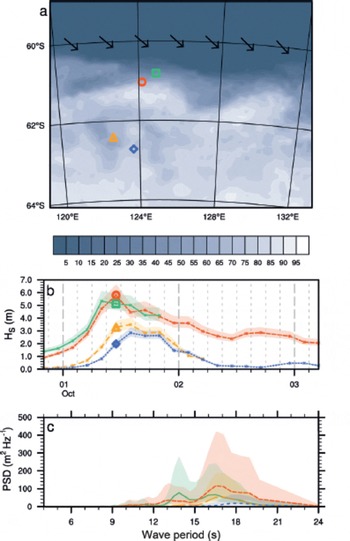
Fig. 11. Same as Figure 8, but for data from 1 October 2012 at 11.00.

Figure 12 is another example of a non-straightforward case. During this event, the wave hindcast calculated westerly swell (Fig. 12a), perhaps explaining why the peak wave height of the deepest WIIOS (diamond) occurred before the peak of the northernmost WIIOS (circle, Fig. 12b). Also unexpected is that the peak period of the deepest WIIOS (dotted) is less than the peak period of the northern WIIOS (dashed, Fig. 12c).

Fig. 12. Same as Figure 8, but for data from 8 October 2012 at 23.00.

These figures highlight the complexities associated with calculating the wave decay at individual frequencies, due to its direct relationship with location, wave direction and ice conditions. For future measurements, it would be beneficial to record the waves continuously, rather than only every 3 hours, in order to track the peaks of each event. We conclude that more data and further analysis are required to conclusively explain the spectral evolution of waves through sea ice.

We also show the spectra from one WIIOS evolving from a growing sea (wave energy (spectra) growing) to a reducing sea (wave energy decaying) (Fig. 13). Here we see the widening spectrum and the peak period increase during a growing sea (solid–dashed). In a reducing sea (dashed– dotted), the wave appears to lose energy evenly across the spectrum (Fig. 13c).

Fig. 13. (a) The location of the WIIOS (markers) on 23 September 2012 at 14.00, 17.00 and 20.00 with ice concentration (%) contours. (b) The significant wave heights, H _s, over time. (c) The PSD on 23 September 2012 at 14.00, 17.00 and 20.00. The circle, square and triangle markers correspond to the 23 September 2012 at 14.00, 17.00 and 20.00, respectively. The shaded regions in (b) and (c) give the 90% confidence intervals.

Summary/Discussion

Five waves-in-ice observation systems (WIIOS) were deployed on Antarctic sea ice during SIPEX II. In this paper, we present the hardware and software details of each WIIOS and an overview of the returned dataset.

The key sensor within each WIIOS was a high-resolution vertical accelerometer. The raw accelerations were oversampled at 640 Hz. A low-pass filter was applied with a cutoff at 0.5 Hz, and the time series was decimated down to 2 Hz. The data were integrated and a high-pass filter applied to obtain displacement. The PSD was then calculated via Welch’s method, using a 10% cosine window and detrending on four segments with 50% overlap. The processed and compressed data were then returned via the Iridium satellite system.

Of the five WIIOS, only one survived the expected lifetime of the WIIOS (6 weeks). The other four stopped transmitting during storms, the first after only 20 hours and the others during subsequent large wave events. In total, we collected 17.5 days of data which can be used to approximate wave decay. The majority of waves measured were during calm seas. Within 100 km of the ice edge, the majority of significant wave heights were 1–2 m and the peak period 10–12 s. Overall, the significant wave height decayed and the wave period lengthened as they propagated beyond 100 km from the ice edge, with the majority of significant wave heights decaying to 0 –1 m and the peak periods lengthening to 14–16s. In addition, several large wave events were measured. We examined a few examples of these in terms of alignment with wave direction and ice extent, and found that to accurately measure the spectral evolution of waves decaying in sea ice, a detailed description of the wave direction and the sea ice is required. To conclusively study the spectral evolution of wave decay in sea ice, returning the directional wave spectra, surveying the ice field before and after each event and measuring the data continuously to capture the arrival times of each peak more accurately would be valuable. Our analysis shows that on occasion, instead of the wave energy simply decaying at each wave period, the energy can cascade, causing more energy than expected at longer periods.