


Introduction
The Wilkins Ice Shelf (WIS) is located in the southwestern part of the Antarctic Peninsula, occupying an embayment between Alexander, Rothschild, Charcot and Latady islands. In early 2008 it had an area of 13 000 km2. Two studies, largely based on remote-sensing data, have given insight into the dynamic character of this ice shelf: Reference Vaughan, Mantripp, Sievers and DoakeVaughan and others (1993) suggested that the mass balance of the WIS was determined largely by surface accumulation and basal melting, and that as a consequence it might be particularly prone to variations in atmospheric and oceanic temperature. Radio-echo soundings indicated that much of the ice shelf was saturated with water. A significant number of tiny ice rises had not led to severe damage, and the calving front was generally free of rift systems. This, together with low rates of ice flow, was taken to indicate that the state of the ice shelf was relatively stable at that time. However, remote sensing of the calving fronts in the early 1990s indicated that the northern ice front had begun to retreat (Reference Lucchitta and RosanovaLucchitta and Rosanova, 1998). This process accelerated during the late 1990s, and a major calving event in 1998 (Reference Scambos, Hulbe, Fahnestock and BohlanderScambos and others, 2000) was a precursor to the most dramatic losses the WIS experienced in the subsequent decade. Increasing basal melt rates, due to variations in the ocean regime, and changes in the material properties, due to atmospheric and oceanic changes, were suggested as possible sources for the reduced integrity of the ice shelf (Reference Braun and HumbertBraun and Humbert, 2009).
During 2008, the WIS experienced major mass loss in three distinct break-up events (Reference Humbert and BraunHumbert and Braun, 2008; Reference Braun and HumbertBraun and Humbert, 2009; Reference ScambosScambos and others, 2009). Two of these occurred along the northwestern ice front between Charcot and Latady Islands. After these break-up events, and the smaller losses that followed soon after, a narrow portion of ice shelf was all that remained between the southern ice shelf and Charcot Island. We describe this as the ice bridge, with a width of only 900 m at its narrowest part. Figure 1 shows the location of the WIS and the shape of the ice bridge at this time. Across the ice bridge, ice thickness varied from 200 to 250 m (Reference Braun, Humbert and MollBraun and others, 2009). By the summer of 2008/09, the imminent failure of this ice bridge was expected and we were of the opinion that its geometry was unlikely to sustain an appreciable load for very long. However, the ice bridge remained intact for more than 9 months, before it finally failed early in April 2009.

Fig. 1. Map of the northern part of the Wilkins Ice Shelf (large image) superimposed on a TerraSAR-X ScanSAR image of 22 February 2009. The insets show the location of the study area on the Antarctic Peninsula (upper) and on the WIS (lower). The blue arrows highlight rifts perpendicular to the ice bridge, mentioned in the text. The ice-front positions in 1990 and prior to the break-up events in 2008 are marked in orange and red, respectively. DLR: Deutsches Zentrum für Luft- und Raumfahrt; ESA: European Space Agency; ASAR: advanced synthetic aperture radar.
The aim of this study is to investigate the deformation of the ice bridge before and during its failure. To achieve this, we analysed high-resolution imagery acquired by the X-band high-resolution synthetic aperture radar TerraSAR-X and data from a GPS (global positioning system) receiver installed on the ice bridge in January 2009.
Deformation of the Ice Bridge
Terrasar-X Data
We used high-resolution TerraSAR-X stripmap-mode images (processed to 3 × 3 m pixel spacing), geolocated using high-precision orbit parameters (leading to sub-pixel position accuracy; M. Eineder and T. Fritz, http://www.geosolutionconsulting.net/uploads/media/Product_Guide.pdf), to measure horizontal displacements of the margins of the ice bridge to a precision of a few tenths of metres. The available images allowed us to build a time series beginning only weeks (29 June 2008) after the ice bridge was formed (Fig. 2) and ending with an image acquired on 4 March 2009. The ice-front positions were identified manually, and limited to the set of images acquired with the same viewing geometry. Figure 2 shows the location of the margin of the ice bridge on 29 June 2008 (red) and 4 March 2009 (blue). Positions of the margins at other dates (we analysed 8 out of 13 very high-resolution TerraSAR-X stripmap-mode images) are not shown but were used in our evaluation of the bridge response. The accuracy of manually identifying the location of the margin is ∼3 pixels.
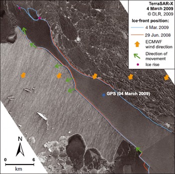
Fig. 2. Deformation of the ice bridge. The ice-front positions on 29 June 2008 (red) and 4 March 2009 (blue) are superimposed on a TerraSAR-X stripmap-mode image of 4 March 2009. The arrows indicate the direction of the movement. Ice rises are marked in purple. The orientation of the surface roughness of the open ocean southwest of the ice bridge represents the wind direction. High winds were indicated by re-analysis data.
The general pattern of the deformation of the ice bridge prior to failure can be divided into three regions. The northernmost part, towards Charcot Island, shifted in a northwesterly direction, with a left-lateral shear rift pattern along the eastern edge of Charcot Island. At the same time, the narrowest part of the ice bridge was being deflected westwards by bending. The southernmost part moved north parallel to the long axis of the ice bridge. The narrowest part of the ice bridge seems to have acted like a hinge and experienced the highest strain. The arrows in Figure 2 show the direction of the movement as determined from the TerraSAR-X imagery using easily identifiable features on the ice shelf. The figure also shows the position of two ice rises that caused the build-up of compressive stress in the northern part of the ice bridge.
Comparison between the ice-front positions on 29 June and 29 August 2008 revealed that some deformation was already in progress. At that time, the ice melange in the northeast of the ice bridge did not appear to be compacted and was probably not exerting stress on the bridge. Thus, we infer that the deformation of the ice bridge at this time was due to ice creep within the ice bridge itself and the flow from the centre of the WIS into the ice bridge.
After the end of August 2008, the ice melange closed up and remained well packed until the end of January 2009 (Envisat and TerraSAR-X images which are not shown here). The ice melange, consisting of mixed icebergs with heights of 10 m and sea ice, had a high surface roughness. This suggests that the surface wind would exert considerable drag on the ice melange. As shown in Figure 2, the patterns of open water on the western side of the ice bridge indicate that the predominant wind direction in this area was from the north-northeast. After January 2009 the ice melange temporarily opened and leads formed, allowing the ice melange to become more mobile.
GPS station data
A single-frequency (L1) GPS receiver, developed at the Institute for Marine and Atmospheric Research Utrecht (IMAU) for continuous remote measurements (Reference Van de WalVan de Wal and others, 2008), was deployed on the ice bridge on 19 January 2009. The receiver was equipped with batteries for unmanned operation over several years, if necessary. The receiver was mounted on a single stake, fixed 1.5 m into the snow surface. Position data were recorded by the GPS every 3 hours, each with an accuracy of 1 m, and were transmitted every 6 days via the Argos system. A substantial limitation of these data is the lack of base-station corrections. However, given the relatively high deformation rates of the bridge, these raw positions remain valuable. After removal of incidental outliers, the positions were used to calculate ice-shelf motion. A small tidal influence was observed in the horizontal displacement, but is not discussed here.
The wind data shown in Figure 3c (bottom panel) were derived from 6 hourly operational analyses of 10 m wind speed and direction, from the weather forecasts produced by the European Centre for Medium-Range Weather Forecasts (ECMWF). These analyses are generated as the best possible estimate of the state of the atmosphere at the moment of generation, and are used as the starting point for operational weather forecasting. Their generation requires assimilation into the ECMWF high-resolution model, using four-dimensional variational data-assimilation techniques, of all observations from the Global Telecommunication System, which includes station, balloon, ship and several satellite observations. The native resolution of this model is 0.25˚ at the Equator; the data presented here have been interpolated to 0.2˚ resolution. The colour in Figure 3c denotes the wind direction. The 2 m wind measurements from Rothera Station are also shown (upper panel of Fig. 3c). Rothera Station is 250 km away and measures wind speeds at a lower height, which may explain some of the differences between the records.
Fig. 3. (a) Absolute velocity of the GPS station prior to the failure. The peaks were correlated with storms. (b) Cumulative displacement as recorded by the GPS station. (c) Rothera and ECMWF wind direction (colour) and velocity from 19 January to 31 March 2009.
Over the period 19 January to 31 March 2009 (before collapse of the ice bridge) the GPS receiver moved 114 m in the west-southwest direction, with a mean velocity of 1.6 m d−1 (587 m a−1). However, during this period, large variations in velocity took place, as can be seen in Figure 3a. In particular, there were a few events during which the velocities increased rapidly. After each of these, the station partly recovered its position, probably as a result of the elastic rebound of the ice bridge (Fig. 3b). These events were apparently correlated with storms shown in the wind records of Rothera Station. The periods when the GPS moved most were correlated with strong northerly winds apparent in both wind datasets. Other peaks in the wind speeds, not correlated to large GPS speeds, occurred when the wind direction was not able to exert pressure on the ice bridge.
These large increases in the GPS velocity observed during storms were unlikely to have resulted solely from the action of the wind on the vertical faces of the ice bridge. We believe it is more likely that the transmission of the wind force via the ice melange, due to its high surface roughness, enhanced the effect of the wind on the ice bridge. The ice-velocity minima seen in Figure 3a on 17 February (the wind direction changed towards the north on this date; Fig. 3c) and 21 February (analogous to backward-oriented displacement in Fig. 3b) are correlated to dates of an un-solidified melange. Figure 1 shows a large part of the ice melange, including leads, in a TerraSAR-X scansar image of 22 February 2009, a date correlated to easterly movement of the GPS station.
We thus infer that the pressure that the melange exerts on the ice bridge contributes considerably to the deformation of the ice bridge in two ways: (1) a periodic enhancement of the wind effect and (2) a monotonic component arising from expansion and strengthening of the ice melange. We conclude that there are three components of ice deformation: (1) a component arising from ice creep of the ice bridge; (2) a monotonic, partly reversible component arising from the ice melange; and (3) a non-monotonic, partly reversible component due to wind.
Failure of the Ice Bridge
Temporal evolution of the disruption
The data discussed above suggest two scenarios for the failure of the ice bridge: (1) growing rates of deformation eventually exceeded a critical limit at the narrowest part of the ice bridge, such that a crack was forced to propagate and the ice bridge became separated from the central WIS; or (2) transient stresses induced by a storm exceeded the critical limit, with the same consequence.
At the end of March 2009, a set of rifts oriented perpendicular to the long axis of the ice bridge began to propagate (blue arrows in Fig. 1), indicating that failure was imminent. The failure began with formation of new cracks on 1 April 2009, as can be seen in the TerraSAR-X stripmap-mode image shown in Figure 4a. The figure highlights the first cracks forming along the long axis of the ice bridge; this was followed by the release of a few small icebergs.

Fig. 4. Temporal evolution of the failure of the ice bridge. (a) TerraSAR-X stripmap-mode image of 1 April 2009 (00:56 UTC). The red curves denote the initial cracks. (b) Envisat ASAR image of 2 April 2009 (5:18 UTC). (c) Envisat ASAR image of 4 April 2009 (12:29 UTC). (d) TerraSAR-X stripmap-mode image of 6 April 2009 (01:05).
An Envisat advanced synthetic aperture radar (ASAR) image acquired on 2 April 2009 (05:18 UTC) showed that several cracks had appeared in the southern part of the ice bridge, parallel to its long axis (Fig. 4b). A second image acquired on the same day (at 11:52 UTC) revealed that the first icebergs had already separated by this time. These observations are consistent with GPS data, which recorded a displacement of 393 m between 2 and 3 April.
The fracture pattern observed in these images suggests the following reason for the occurrence of these cracks. The fracture pattern and the fragments suggest that a preexisting damage texture was present. Consequently, the structural integrity of the southwestern part of the bridge suffered. The damage situation can be thought of as a fibre-like structure. As this fibre-like structure is prone to buckling under compressive axial loads, the break-up event depicted in Figure 4c and d initiated in this region. Given the large undamaged part in the northeast of the bridge, the only possibility is for the fibres to buckle into the open sea on the southwest. Thus, disintegration must have been accompanied by compressive stresses along the bridge axis in the southwestern region, shown in Figure 5. The origin of the compressive stress state is most likely two-fold. At first, the flow of the ice along the bridge is decelerated from the southwestern base (inflow) to the narrowest part. This deceleration is associated with compressive stresses across the bridge width. Secondly, as the narrowest part acts like a hinge, a bending-type deformation of the bridge is observed. This bending induces stresses with varying intensity and sign across the width of the bridge. Due to the bending to the southwest, compressive stresses occurred at the southwestern edge of the bridge. Pure bending would induce tensile axial stresses at the northeast boundary of the bridge. The distribution of axial stresses is sketched in Figure 5. The superposition of the two compressive stress states in the southwestern part explains the buckling-type disintegration of this part of the bridge.

Fig. 5. Stresses and loads on the ice bridge. This figure is based on Figure 2 with superimposed stresses and load. The black arrows characterize schematically the load situation along the eastern ice front, arising from the ice melange. Red arrows denote stresses due to deceleration, blue arrows stresses due to bending.
An Envisat ASAR image of 4 April 2009 (5:55 UTC) (Fig. 4c) shows that the southern part of the ice bridge released scores of icebergs and the northern part of the ice bridge became entirely ruptured. Figure 4d shows a TerraSAR-X stripmap-mode image of 6 April 2009 that indicates the final state of disruption. The size of the disrupted area is –330 km2.
After the failure of the bridge, the GPS unit continued its journey on an iceberg originally ∼5 km long and 500 m wide. Between 2 April and 23 May the iceberg drifted ∼100km in a southwesterly direction towards the open ocean before it finally drowned on 3 August 2009 (Fig. 6).

Fig. 6. Drift of the iceberg carrying the GPS station, after the failure of the ice bridge, superimposed on an Envisat ASAR wide-swath image from 1 to 3 August 2009.
Released energy
In order to assess the energy released during the failure of the ice bridge, the area of the newly formed iceberg surfaces had to be determined. For this purpose, the perimeters of both upright and capsized icebergs were measured using a TerraSAR-X stripmap-mode image from 6 April 2009. Only new side-walls of icebergs that originated along the former ice front were taken into account. Capsized icebergs were assumed to have the maximum width according to the floatation stability criteria. Approximately 75% of the newly formed area originated from upright icebergs, while ∼2 5% was due to capsized icebergs. Since the determination of the area is hampered by image resolution and ice thickness, we only consider a lower limit. Assuming an ice thickness of 200 m, we estimate the newly formed surface to be 150 km2.
The energy release rate, G, during mode I or mode II cracking, when the fracture criterion is fulfilled, is given by
with K Ic and K IIc the fracture toughness for mode I and mode II, respectively, and E the Young’s modulus (Reference Gross and SeeligGross and Seelig, 2006). We assume that the fracturing was either mode I or mode II and that K Ic ≈ K IIc = 125 kPam0.5 (Reference Schulson and DuvalSchulson and Duval, 2009), so Equation (1) reduces to
The Young’s modulus of ice is assumed to be –933 MPa (Reference Schulson and DuvalSchulson and Duval, 2009). These estimates imply an energy release rate, G = 1.675Jm-2. This is defined as energy release per unit crack advance, which implies the formation of two new opposite surfaces. Assuming a homogeneous energy release rate and neglecting possible existing pre-cracks or damaged zones, the amount of energy, ΔE, released during the fracturing event can be estimated from the area, A = 150 km2, of the newly created surfaces during the failure by
This energy release is equivalent to ∼2 7 kg of TNT, and represents a lower limit. While this energy had to be raised by the system before cracking could take place, energy release due to capsizing icebergs was not related to the cracking process itself. Iceberg capsizing leads to a release of potential energy, as the denser ocean water moves to a lower potential level. The energy balance can be written as
where the subscripts ‘pot’ and ‘kin’ indicate potential and kinetic energy, respectively, and ‘prior’ and ‘post’ refer to before and after capsizing. The kinetic energy of the capsized icebergs can be split into
where ![]() is the rotational energy during the capsizing and
is the rotational energy during the capsizing and ![]() s the energy that goes into translational motion of the capsized icebergs. The kinetic energy of the ocean consists of the following components:
s the energy that goes into translational motion of the capsized icebergs. The kinetic energy of the ocean consists of the following components:
with ![]() iaens the kinetic energy of eddy formation
iaens the kinetic energy of eddy formation ![]() the kinetic energy available for formation of waves (e.g. tsunamis). The energy balance, Equation (4), then becomes
the kinetic energy available for formation of waves (e.g. tsunamis). The energy balance, Equation (4), then becomes
with A s the surface area of the capsizing icebergs, H their thickness, ρice the density of ice, ρ sw the density of sea water, b the width of the capsized iceberg and g the gravitational acceleration. The left-hand side of this equation is due to Reference MacAyeal, Okal, Aster and BassisMacAyeal and others (2009), who discussed generation of seismic waves and tsunamis by capsizing icebergs during the February and May 2008 break-up events. Assuming a thickness of 200 m, the capsizing icebergs have a width b ≤ 156 m. The determination of the capsized area from satellite imagery is limited, as only the lengths of the capsized icebergs are visible. Thus, we assume here a lower limit of 22 km2 and an upper limit of 34 km2 for As. The released energy ranges between 1 and 6 × 10¹⁴ J, assuming a lower limit of b = 20 m, which is much larger than the energy release by fracturing. Although a large number of satellite images exist, we are, as yet, unable to determine single terms of the right-hand side of Equation (7), so it remains unclear which amount of energy is accessible for the generation of large waves.
Conclusions
We have described the deformation and ultimate failure of the ice bridge on the WIS. The spatial deformation of the ice bridge was assessed using the high resolution and unprecedented geolocation accuracy of TerraSAR-X stripmap-mode imagery, while the temporal variations were effectively measured using GPS. The deformation of the ice bridge was largest at the narrowest part, which bent towards the west and acted like a hinge. The deformation consisted of monotonic and periodic, partly reversible components. We believe that the reversible component was caused by several distinct storm events. However, the strain due to storm events was not entirely elastic: the strain was not completely recovered after the storm had abated. Similarly, we believe that the monotonic component was largely the result of ice creep as well as being due the ice melange.
The failure of the ice bridge began on 1 April 2009 and proceeded until 4 April 2009. The southern part shattered into >100 tabular floating icebergs and numerous capsized ones. We suggest that the calving of these icebergs was facilitated by a pre-existing damage texture in the ice shelf. The consequence of this texture, analogous to a bundle of fibres, was that it buckled under compressive stresses, and the structural integrity of the ice bridge was lost.
The newly formed surfaces generated during the failure of the ice bridge amounted to at least 150 km2. This increase in surface area implies an energy release of at least 125×106 J, equivalent to 27 kg of TNT, which gives an idea of the energy stored in the ice prior to the collapse of the ice bridge. Subsequently, potential energy ( 10 14 J) was released as icebergs capsized. This available energy can be transformed into kinetic energy of the icebergs, eddy formation and wave generation. However, the observations do not allow a precise estimate of the period over which this energy was released.
Finally, we note that, while this study shows that the deformation and failure of the ice bridge can be described in detail, and many aspects are understood in terms of the broad processes involved, this ice bridge was undoubtedly unique and it may not be possible to draw wider conclusions about ice-shelf break-up in general; this may only be achievable after similarly detailed analysis of several similar events.
Acknowledgements
The TerraSAR-X images were provided by the German Aerospace Center (DLR) under proposal LAN0013. We thank R. Metzig (DLR) for support in acquiring the TerraSAR-X images. The Envisat ASAR images were provided by the European Space Agency (ESA) under proposal ESA IPY AO 4032. We acknowledge the British Antarctic Survey logistics for deploying the GPS equipment. R.M. and M.B. were supported by the German Research Foundation (DFG) under grants MU 1370/4–1 and BR 2105/8–1, and D.G.V. was funded by the Natural Environment Research Council. We thank T. Scambos and F. Pattyn for helpful comments.


