


Introduction
Global data sets collected from spaceborne sensors are a principal component of global change studies. Indeed, several types of spaceborne data are becoming sufficiently extensive, both spatially and temporally, so as to provide important measures of global change. Obviously, if those data sets are to fulfill their promise, careful calibration and validation are essential over the life of individual sensors used to acquire the data (e.g. Reference Cavalieri and SwiftCavalieri and Swift, 1987; Reference Comiso and ZwallyComiso and Zwally, 1989). It is equally important to provide for cross-calibration between a succession of similar sensors when long baselines of observations are required.
Data from NASA's Scanning Multichannel Microwave Radiometer (SMMR), followed by the Navy's Special Sensor Microwave Imager (SSM/I) (Reference Hollinger, Lo and PoeHollinger and others, 1987), as well as predecessor instruments, such as the Electrically Scanning Microwave Radiometer (ESMR), provide an opportunity for a case study of the issues faced by the earth science community when attempting to establish long base-line data sets. Data from each of these passive microwave instruments are separately and routinely processed to derive estimates of sea-ice concentration and multi-year ice fraction (e.g., Reference Zwally, Comiso, Parkinson, Campbell, Carsey and GloersenZwally and others, 1983). Along with operational utility, sea-ice geophysical products from SMMR are being studied extensively for trends in total and hemispheric ice concentrations that would serve as evidence for changes in global temperatures. For example, SMMR observations of sea-ice extent and open water areas show a significant decrease in the Arctic, whereas no significant trends were observed in the Antarctic (Reference Gloersen and CampbellGloersen and Campbell, 1991). Also, time series of SMMR brightness temperature data have also been used to investigate relative trends in surface physical temperature for different sectors of the Antarctic ice sheet. Along with strong seasonal trends, those data reveal important differences in the timing of temperature anomaly events between East and West Antarctica (Reference Jezek, Cavalieri and HoganJezek and others, 1990).
It is natural to attempt combining data from successive satellite programs into a single, long record of measurable geophysical variables. Two approaches are possible, the first being to “match” values of a derived variable obtained near the end of one sensor's useful life with values obtained near the beginning of the follow-on sensor's mission. A second approach is to compare lower level data products and develop a procedure for relative calibration. This latter method is adopted here. Gridded brightness temperatures are compared during the brief overlap between SMMR and SSM/I sensors for the Antarctic ice sheet. Linear regressions are computed using complementary pairs of channels. A calibration scheme was derived and applied to a subset of the SMMR and SSM/I data.
Approach
Data sets used in this study were gridded SSM/I brightness temperature data obtained on CD-ROM from the National Snow and Ice Data Center (NSIDC, 1990; Reference Swift and CavalieriWeaver and others, 1987). Gridded SMMR total calibrated temperature (TCT) data for the overlap time period between the SMMR and SSM/I sensors were obtained from the Goddard Space Flight Center (Reference Gloersen, Campbell, Cavalieri, Comiso, Parkinson and ZwallyGloersen and others, 1992). (The SMMR data used are the latest recalibrated data sampled to the SSM/I grid.)
Only complementary pairs of channel were compared, namely the SMMR 18V, 18H, 37V, 37H and SSM/I 19.35V, 19.35H, 37V and 37H channels during the period of overlap. The period of overlap began on 11 July 1987 and lasted until 20 August 1987. Because SMMR acquired data every other day, this resulted in 20 days of nearly simultaneous observations by both sensors.
Initially, the SMMR and SSM/I gridded data were compared by simply differencing like channels. Raster images of difference maps revealed strong differences in the vertical channels (−14 to +10K) and lesser differences in the horizontal channels (only a few K). Patterns in temperature differences closely mimicked the spatial patterns in the original brightness temperature data for the vertical channels. Spatial patterns evident in the brightness temperature data for the horizontal channels were mostly absent in the difference maps.
Several hypotheses were tested to explain these results. Because of the proximity of the SSM/I 19.35 GHz channels to the 22 GHz water vapor absorption line, we first assumed that water vapor in the atmosphere might be causing the spatial patterns of brightness-temperature differences between the lower frequency SMMR and SSM/I channels. However, we observed similar spatial patterns in the difference maps of the 37 GHz channels, thus refuting the importance of water vapor.
The pointing angles of the two instruments are different (SSM/I points at 53.1°; SMMR points at 50°). A second hypothesis was developed to test the effect of differing angles of incidence. This seemed a promising hypothesis because the pointing angles are close to the Brewster angle for polar firn. This fact would argue for the stronger spatial variations in the vertical channels, as compared to the horizontal channels, that were observed in the difference maps. However, simple Fresnel reflection coefficient calculations using typical values for the density of polar firn (0.35 to 0.5 Mg m−3) showed that the angle of incidence differences account for less than 1 K of variation.
The remaining hypothesis was simply to allow for variations in the relative offset and gain between the various channels. A purely additive offset would account for much of the difference, while a multiplicative gain difference would explain the observation that patterns in brightness temperature were preserved when differences in brightness temperature were mapped.
We tested this hypothesis by correlating the SMMR and SSM/I gridded brightness temperature data during the overlap period. A distinct correlation was observed between data from each pair of complementary channels. The correlation was obviously complicated by unex-plained factors that caused large variances in the comparison. To improve the analysis, we next limited the data geographically to include observations taken only from over the Antarctic ice sheet. Ocean and sea-ice data were masked out to avoid the complexities of the temporally, more volatile, seaward conditions. An example of the correlations for the four pairs of channels for the first and last day of overlap for only the ice sheet area are shown in in Figures 1 and 2 (all correlation plots for the 20 d of overlap are presented in Reference JezekJezek and others, 1991).
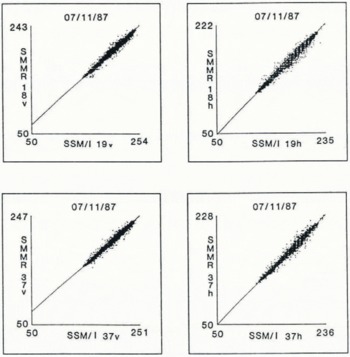
Fig. 1. Regression plots for the four pairs of complementary channels. Data are from the first day of overlap between the two sensors (7 July 1987). Only data taken over the Antarctica ice sheet are included.

Fig. 2. Regression plots for the four pairs of complementary channels. Data are from the last day of overlap between the two sensors (20 August 1987). Only data taken over the Antarctica ice sheet are included.
Results
A linear regression of the form
was applied to each correlation plot, where g is the slope of the regression line, dc is the intercept and SMMR(Tb) and SSM/I (Tb) are the values of brightness temperature. Slopes and intercepts for each pair of data were calculated (see Reference JezekJezek and others, 1991). Figures 3 and 4 show the slopes and intercepts for each pair of channels, plotted as a function of time. Because there is no consistent trend in the time series values of slopes and intercepts, we feel justified in computing average values of the slopes and intercepts for the channel pairs. These are given in Table 1.
Table 1. Average slopes and intercept values determined by a regression between SMMR and SSM/I brightness-temperature data collected over the Antarctic ice sheet

We identified three major concerns with our analysis: the time of collection, geolocation, and sky radiation. SSM/I and SMMR data were not collected simultaneously and there is as much as a 6 h difference between observation times. We do not consider this a serious problem for data taken over the ice sheet for two reasons. At the lower frequencies, several meters of firn contribute emitted energy and the temperature response of that bulk layer of snow to reasonable changes in air temperature over a period of several hours is likely to be small (a degree or two at most). Air temperature variations may affect the interpretation of the higher frequency data, but temperature records acquired from automatic weather stations at several locations in Antarctica indicate that diurnal variations over much of the continent during the dead of winter are only a few degrees (data from Automatic Weather Station Program, University of Wisconsin-Madison).

Fig. 3. Slope values derived from the regression analysis for each pair of complementary channels during each day of overlap.

Fig. 4. Intercept values derived from the regression analysis for each pair of complementary channels during each day of overlap.
During the early part of the SSM/I mission, a gcolocation problem was discovered with a magnitude of 25 km or about 1 pixel. We have not attempted to improve the co-registration of the data, primarily because the gradients in brightness temperature across the ice sheet are on an average less than 2 K per pixel, although in some coastal areas and in mountainous areas, the gradient can be as high as 5 K per pixel. We note that increased brightness temperature gradients and a stronger diurnal cycle of physical temperature change near the coast may explain the slight broadening of the variances about the regression lines at higher brightness temperatures. There is some suggestion (Figs 1 and 2) that the variances at higher temperatures increase with time, possibly coinciding with the seasonal lengthening diurnal cycle.
Finally, there may be a diurnal difference in the amount of atmospheric radiation emitted directly to the sensors and reflected off the surface that might corrupt the regression of non-simultaneous data. We do not measure strong trends in the regression coefTicients during the overlap time period even though the average surface air temperature in August, 1987 at Byrd Station was 7°C cooler than in July and about 4°C cooler at Dome C. Consequently, we do not believe that sky radiation is an important issue in this analysis.
Figures 3 and 4 demonstrate that the slopes of regression lines are significantly different from unity and that the intercepts are significantly different from zero. In fact, the intercepts can be quite large, exceeding 30 K for the 37v channel comparison. It seems reasonable to ask why such apparently large offsets would go unnoticed during the initial inspection of each data set. The answer lies with the fact that the relative difference between SMMR and SSM/I brightness temperatures changes with the magnitude of the temperature. That point is demonstrated in Figure 5 where predicted differences are plotted as a function of SSM/I brightness temperature. The functions plotted in Figure 5 are derived from the regression analyses and the equation
Using Figure 5, it can be seen that in the SSM/I temperature range from 150 to 250 K, corresponding deltas span a range from about + 10 to −10 K, depending on the channel. Thus, while the differences at these temperatures may be reduced relative to the intercept values, geophysical analysis at only these temperatures would tend to overlook the details of the relative calibration differences.

Fig. 5. Differences between SMMR and SSM/I brightness temperature data predicted using the regression coefficients listed in Table 1 when compared to the SSM/I brightness data.

Fig. 6. Mean monthly values of brightness temperature for the ice domes area from the SMMR and SSM/I data sensors.

Fig. 7. Mean monthly values of corrected SMMR and SSM/I brightness temperatures for the ice-domes area.
We next examined data averaged over a sector of East Antarctica to test the calibration coefficients derived from the SMMR and SSM/I data sets. This area was the focus of prior work by Reference Jezek, Cavalieri and HoganJezek and others (1990) with SMMR data and is named the Ice Domes region in their Figure 1.
Daily brightness temperature values were extracted from the 19.35 v, 19.35 h, 37 v and 37 h SSM/I channels. The daily values were averaged on a monthly basis to compare with earlier SMMR monthly data. The entire series of monthly brightness temperatures from the SMMR and SSM/I sensors are shown in Figure 6 (January 1979 through June 1990). Gridded SMMR data for 1986 were unavailable at the time of our study. Seasonal variations in the SMMR and SSM/I data are broadly similar, however, there is a large offset between the SMMR and SSM/I data. The SMMR data were then adjusted using the calibration coefficients in Table 1. The results are shown in Figure 7, which demonstrates that the calibration eliminates the offset.
Discussion
Brightness temperatures are strongly modulated by the seasonal changes in physical temperature over the entire data set (Fig. 7). The coldest brightness temperatures occur between months 42 and 46 (June through October, 1982) and coincide with the 1982 El Niño event as previously noted in Reference Jezek, Cavalieri and HoganJezek and others (1990) (Fig. 8).
Unlike the unadjusted SMMR data (Fig. 6), Figure 7 shows that the 18 GHz vertical channels tend to fall within the 37 GHz envelope. This is to be expected because the lower frequency channels average over a greater depth, thus muting the temperature response of the ice sheet. The 18 GHz horizontal channel tends to be biased towards a lower mean temperature than the 37 GHz horizontal channel. We speculate this may be due to the relatively greater effect of stratigraphy on the reflection coefficient for horizontally polarized waves.
In Figure 8 we plot maximum summer and minimum winter brightness temperatures for each channel. Maximum summer brightness temperatures for the SMMR and SSM/I vertical and horizontal channels occur during January. There is less than a 1 deg increase in average maximum summer brightness temperature for the 37 GHz vertical channel for SMMR, when compared to the 37 GHz vertical channel for SSM/I. The 37 GHz horizontal channels for the two sensors vary in a similar manner. However, there is a 3 deg increase in average maximum summer temperature between the SMMR 18 GHz and SSM/I 19.35 GHz vertical channels. The 18 and 19.35 GHz horizontal channels for the two sensors vary in a similar manner.

Fig. 8. Maximum summer and minimum winter mean monthly brightness temperature for the ice-domes region.
The minimum monthly winter averages for the SSM/I 19.35 GHz channel, when compared to the SMMR 18 GHz channel, increase by 2 deg for both the horizontal and vertical channels. The brightness temperatures for the SSM/I 37 GHz vertical channel also increase by 2 deg when compared to the SMMR 37 GHz; the SSM/I 37 GHz horizontal channel only increases by 1 deg. Nevertheless, there seems to be good continuity across the SMMR and SSM/I time series, particularly for the minimum winter temperatures, which argues against a calibration problem for the two sensors and argues for a short-term trend in physical properties.
Conclusions
Global change monitoring programs must rely on long time series of calibrated data. Regarding observations from space, our analysis demonstrates that overlap between each sensor in a sequence of phased deployments is essential in providing a high level of confidence in at least the relative calibration between sensors.
Acknowledgments
This report was prepared with support from the Polar Oceans and Ice Sheets Program of the National Aeronautics and Space Administration (NAGW-2035) and the Office of Naval Research.


