


1. Introduction
In Greenland and Antarctica, several deep ice-core projects have been carried out during recent decades (Camp Century, Dye 3, GRIP and GISP2 in Greenland; Vostok and Byrd Station in Antarctica) or are currently under way (NorthGRIP in Greenland; Dronning Maud Land, Dome C and Dome Fuji in Antarctica). These ice cores reveal a wealth of direct and indirect information on palaeoclimatic conditions such as atmospheric composition, surface temperature and snowfall rate, going back some hundreds of thousands of years, and have therefore greatly improved our knowledge of Earth’s climate and its variability during the Pleistocene and Holocene (e.g. Reference DansgaardDansgaard and others, 1993; Reference PetitPetit and others, 1999; Reference JohnsenJohnsen and others, 2001).
In order to obtain time series of these climatic parameters, proper age–depth relations for the ice and the boreholes are required. In the upper parts, these can be established rather precisely by counting annual signals of isotopic composition and impurities downward. However, beyond ages of a few tens of kyr these stratigraphic techniques fail due to layer thinning and diffusion, so flow models are needed to compute age–depth profiles in the lower parts of the boreholes (cf. Reference JohnsenJohnsen and others, 2001, and references therein).
Applications of the three-dimensional dynamic/thermodynamic ice-sheet model SICOPOLIS to compute ages for the Greenland Summit (GRIP/GISP2) region were discussed by Reference GreveGreve (1997) and Greve and others (Reference Greve, Weis and Hutter1998, Reference Greve, Mügge, Baral, Albrecht, Savvin, Hutter, Wang and Beer1999), and for Dronning Maud Land (where a deep ice core is planned within the European Project for Ice Coring in Antarctica (EPICA)) by Reference Calov, Savvin, Greve, Hansen and HutterCalov and others (1998) and Reference Savvin, Greve, Calov, Mügge and HutterSavvin and others (2000). In these studies, the present state of the Greenland and Antarctic ice sheets was obtained via palaeoclimatic simulations over two glacial/interglacial cycles, and the three-dimensional age field was computed by solving the advective age evolution equation along with the thickness, temperature and flow-velocity equations. A major limitation in those calculations was the need for some artificial diffusion in the vertical direction in order to achieve numerical stability, which requires an unphysical boundary condition for the age at the ice base. Reference Calov, Savvin, Greve, Hansen and HutterCalov and others (1998) show that this leads to a basal boundary layer of ~15% of the ice thickness in which the computed ages are affected by this arbitrary boundary condition and therefore erroneous.
In this study, we consider a simple one-dimensional steady-state approximation for the age computation. This simplification allows an analytical solution for the age– depth relation against which numerical methods can be checked. After showing a general method to construct numerical solution schemes, we discuss a variety of different schemes in terms of their accuracy and convergence properties.The objective is to find out which scheme is most suitable for applications in full three-dimensional time-dependent simulations in order to provide age fields as precisely as possible over the whole depth of ice cores.
2. Age Equation In Ice Sheets
2.1. General equation
Let us consider an ice sheet in Cartesian coordinates x, y (which span the horizontal plane), z (vertical) and time t. the equation which describes the evolution of the age field A(x, y, z, t) in the accumulation zone of the ice sheet is then
where d/dt is the material time derivative which follows the motion of the ice particles with velocity v = (vx, vy, vz), and z = h(x, y, t) is the free surface of the ice sheet where the ice particles settle as snowflakes. In an Eulerian frame,
where ∂/∂t is the local time derivative. Assuming incompressibility, div v =0, Equation (2) can be written in conservative form as
This equation is of hyperbolic type with a constant source term and a homogeneous Dirichlet boundary condition.
2.2. One-dimensional steady-state approximation
We now assume steady-state conditions and neglect horizontal advection in Equation (2), which is a coarse approximation of the flow conditions in the vicinity of many ice-core positions in Greenland and Antarctica situated on or close to ice domes or ridges (GRIP, GISP2, Dome C, DML05, etc.). Equation (2) then simplifies to
or equivalently in conservative form,
With the scales
where H is the local ice thickness and as is the net accumulation rate, dimensionless quantities ![]() are introduced as
are introduced as
If we choose z = 0 for the local ice base, then for the free surface z = h = H, or ![]() and the dimensionless forms of Equations (4) and (5) become
and the dimensionless forms of Equations (4) and (5) become
In the following, all quantities are taken dimensionless, and tildes are omitted for simplicity of notation.
For the vertical velocity, a Dansgaard–Johnsen type distribution (Reference Dansgaard and Johnsen.Dansgaard andJohnsen, 1969) is assumed, which consists of a constant vertical strain rate ∂vz/∂z from the free surface z = 1 down to a position z = z*, and a linearly decreasing vertical strain rate ∂vz/∂z ∝ z below. With vz(1) = –1 (vertical velocity balances accumulation at the free surface), ![]() (small offset at the base in order to avoid an infinite age) and continuity of vz and ∂vz/∂z at z = z*, this yields
(small offset at the base in order to avoid an infinite age) and continuity of vz and ∂vz/∂z at z = z*, this yields
where
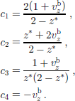
Note that all constants c1–c4 are positive provided ![]() and
and ![]() In the following, we will set
In the following, we will set
The resulting profile is plotted in Figure 1.
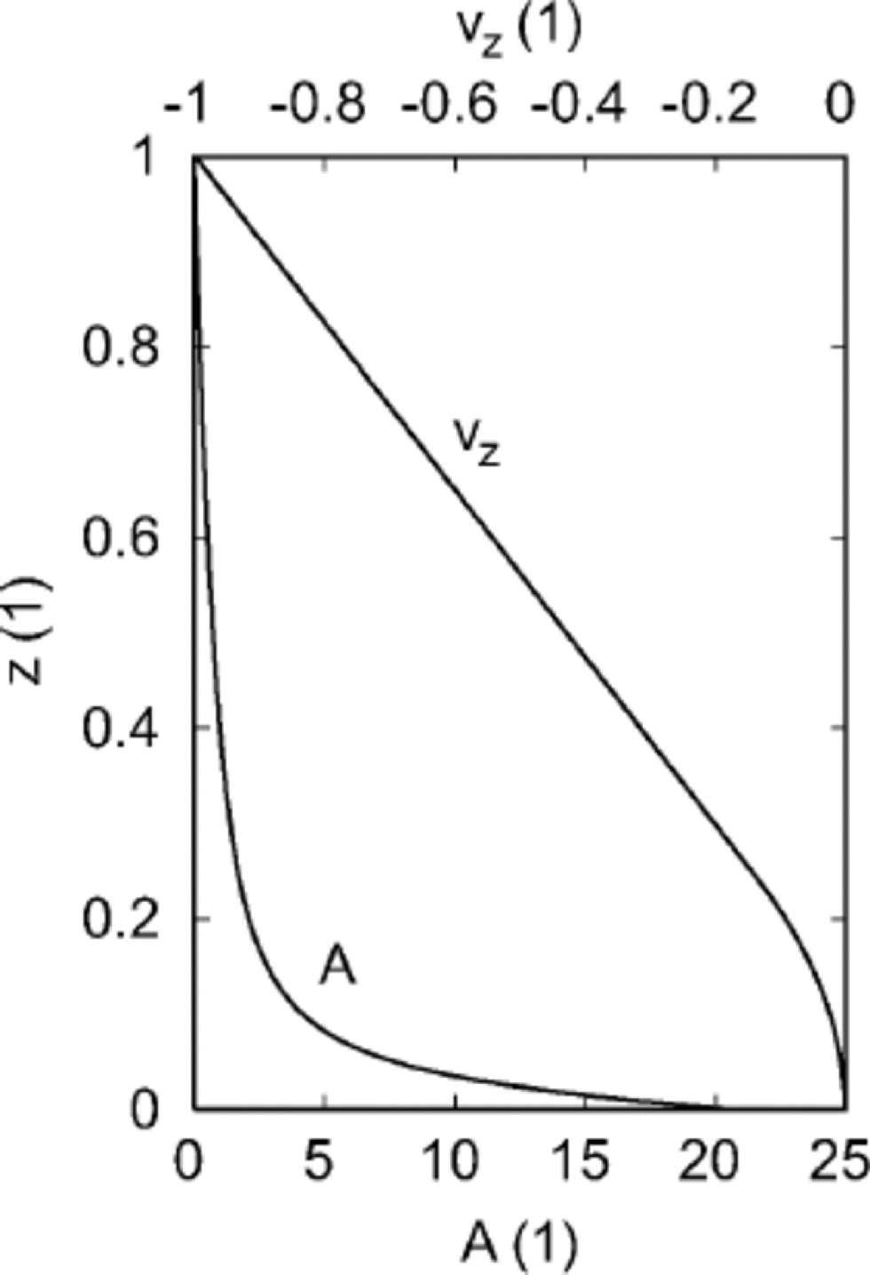
Fig. 1 Analytical profiles of the vertical velocity vz (Equation (9)) and the age A (Equation (12)).
With the velocity distribution (9), an analytic solution of the age Equation (8) 1 can readily be obtained. It reads
This solution is plotted in Figure 1. At the bottom, A = 20.76, which for the GRIP ice core (H = 3028m, as = 0.23m ice equiv. a–1; Reference Dahl-Jensen, Johnsen, Hammer, Clausen, Jouzel and PeltierDahl-Jensen and others, 1993) corresponds to 273.2 kyr. That age is in reasonable agreement with current estimates of about 250 kyr (Reference DansgaardDansgaard and others, 1993; Reference GreveGreve, 1997).
3. Numerical Schemes
3.1. General considerations
We now turn to the numerical solution of the one-dimensional age Equation (8) 2. In order to investigate schemes that can be adopted for non-steady-state conditions, we do not attempt to solve this equation directly, but iterate
with the initial condition A(t = 0) = 0 until steady state is reached. By introducing the flux F and source Q as
Equation (13) can be written in compact fashion,
Let us introduce a discretization of space and time,
where Δz and Δt are the grid spacing and the time-step, respectively, and define averaged ages ![]() fluxes
fluxes![]() and sources
and sources ![]()
Then integration of Equation (15) over the space–time rectangle ![]() in the sense of a finite-volume approach yields the difference equation
in the sense of a finite-volume approach yields the difference equation
which is still exact.
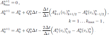
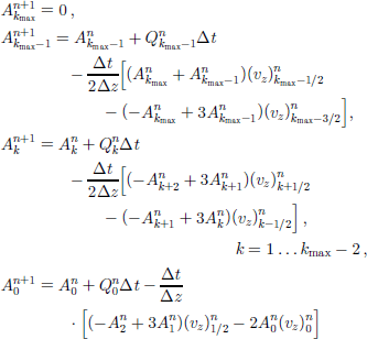
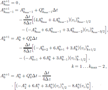
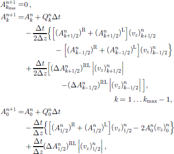
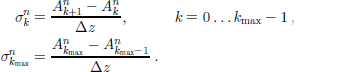
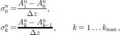
The bottom gridpoint k = 0 needs to be treated separately. Here,
and by integration of Equation (15) over [z0, z1/2]×[tn, tn+1],
Numerical solution schemes can be constructed by assigning approximate values to the averaged quantities in Equations (18) and (20). We will only consider explicit schemes with

where ![]() denote an optional dissipative limiter. Thus, the general iteration rule is
denote an optional dissipative limiter. Thus, the general iteration rule is
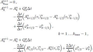
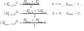
We apply a numerical grid for which the ages A and sources Q are defined on gridpoints (nodes) k, and the velocities vz on cell boundaries k ± 1/2 (staggered grid, Fig. 2). In addition, the basal velocity (at k = 0) is assumed to be known. Therefore, in Equation (22) the ages ![]() do not conform to the grid, and the several numerical schemes derived from Equation (22) differ only in the method of computing the ages
do not conform to the grid, and the several numerical schemes derived from Equation (22) differ only in the method of computing the ages ![]() from neighbouring ages
from neighbouring ages ![]() and in the selection of dissipative limiters
and in the selection of dissipative limiters ![]()
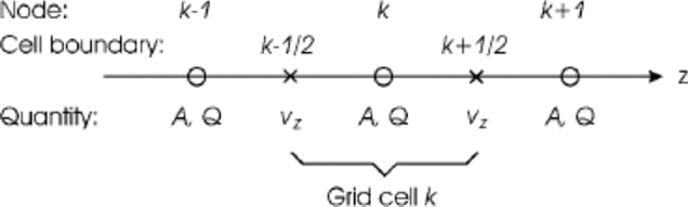
Fig. 2 Staggered numerical grid for the one-dimensional age computation.
3.2. Errors
We assess the error of several solution techniques by comparison with the analytic solution (Equation (12)). Near-basal ice is of particular interest, so we consider the relative error of the basal age,
where A0 is the steady-state basal age of Equation (22) and![]() is the exact analytic value given by Equation (12). We also introduce the relative error for an arbitrary position in the column,
is the exact analytic value given by Equation (12). We also introduce the relative error for an arbitrary position in the column,
Note that, in contrast to ![]() does not contain the sign information because of the logarithmic plotting to be applied.
does not contain the sign information because of the logarithmic plotting to be applied.
3.3. Central differences
The simplest calculation of ![]()
leads to the forward-time central-space scheme (FTCS)
which is of first order in time and of second order in space. However, the resulting iteration is always unstable (Reference Morton and Mayers.Morton and Mayers, 1994). Stability can be achieved by extending the time integration over two time-steps (``leap-frog’’),
which is known as the central-time central-space scheme (CTCS, of second order in time and space). In order to restrict the growth of spurious numerical modes due to decoupling of even and odd iteration steps n, every 101st time-step the CTCS scheme (Equation (27)) is replaced by the FTCS scheme (Equation (26)). This number was found to be sufficient to avoid decoupling. the calculation is also initialized with the FTCS scheme.
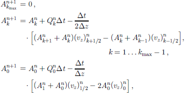
3.4. First-order upstream
The CTCS scheme tends to produce numerical oscillations due to the unphysical central discretization of the advection term. At any point in space, the flow of information is from the upstream direction only. to correct for this, non-central differences pointing in the upstream direction can be used. Schemes of that kind are called upstream (upwind) schemes, 0 and the simplest one is constructed by choosing
For our problem, ![]() (Equation (9); Fig. 1), so that
(Equation (9); Fig. 1), so that
This is the first- order upstream scheme (UP1), which is of first order in time and space.
By subtracting Equations (29)2 and (26)2, one obtains the difference
which corresponds to an additional diffusion term
(numerical diffusivity λnum) on the righthand side of the age equation (15), which is discretized by central differences. the numerical diffusion efficiently dampens numerical oscillations, but a disadvantage is that regions with steep gradients within a smooth solution are smeared out over the spatial domain.
3.5. Second-order upstream
An improvement can be made in the numerical diffusion by replacing Equation (28) with a linear upstream interpolation,
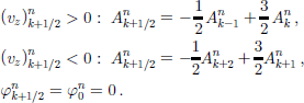
With ![]() and central interpolation for
and central interpolation for ![]() the second-order upstream scheme (UP2)
the second-order upstream scheme (UP2)
is produced. This scheme has first-order accuracy in time and second-order accuracy in space.
3.6. QUICK
Another upstream scheme, the Quadratic Upstream Interpolation for Convective Kinematics (QUICK; Reference LeonardLeonard, 1979), is defined by
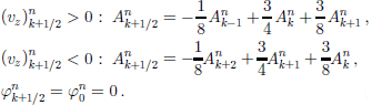
As in UP2, with ![]() and central interpolation for
and central interpolation for![]() the corresponding iteration rule is
the corresponding iteration rule is
This scheme is of first order in time and of third order in space.
3.7. TVD Lax–Friedrichs
The concept of Total Variation Diminishing (TVD) schemes was introduced by Reference HartenHarten (1983). the main idea of TVD methods is to combine the advantages of accurate high-order schemes and dissipative first-order schemes like UP1. This is achieved by introducing a dissipative limiter which ensures that no spurious oscillations develop near a discontinuity or a zone with steep gradients, and high-order accuracy is retained elsewhere. for instance, the solution can be second- or third-order accurate in the smooth parts, whereas the scheme possesses only first-order accuracy at local extrema or discontinuities. In this way only negligible numerical diffusion is introduced, and advection problems even with discontinuities like travelling shock waves can be well modelled. for more details on TVD and related schemes see, for example, Reference YeeYee (1989), Nessyahu andTadmor (1990) and Reference Jiang, Levy, Lin, Osher and TadmorJiang and others (1998).
TVD schemes make use of a piecewise linear reconstruction of quantities within gridcells. for our problem this means that for a gridcell ![]() in place of the single age value
in place of the single age value ![]() as was used in the above schemes (this corresponds to a piecewise constant step reconstruction), a linear reconstruction
as was used in the above schemes (this corresponds to a piecewise constant step reconstruction), a linear reconstruction
is applied. for the slope limiter
![]()
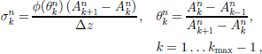
which yields a weighted average of the left-sided and right-sided gradients, and at the boundaries the one-sided gradients
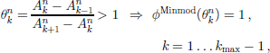
are used. the function ϕ(θ) in Equation (36) must satisfy certain conditions in order to yield second-order-accurate cell reconstructions and satisfy the TVD property (Reference SwebySweby, 1984). We consider three limiters. the Superbee limiter
produces the largest slopes and the smallest numerical diffusion, while the Minmod limiter
produces the smallest slopes and the largest numerical diffusion. the Woodward limiter
lies between those extremes. With all three functions, the slope limiter (Equation (36)) is symmetric with respect to the one-sided gradients ![]() and
and ![]() and vanishes for
and vanishes for ![]()
![]() or sgn n
or sgn n ![]() sgn
sgn![]()
A typical TVD method is the TVD Lax–Friedrichs scheme (TVDLF), defined by
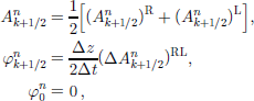
where
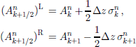
are the values at the cell boundary k+1/2 resulting from reconstruction (35) for the adjacent left (index k) and right (index k + 1) cell, respectively (with either Superbee (TVDLF/S), Minmod (TVDLF/M) orWoodward (TVDLF/ W)), and
A difficulty with the TVDLF scheme is that the dissipative limiter(41)2, which is chosen in analogy to the usual Lax–Friedrichs scheme, results in rather large numerical diffusion. An alternative we therefore also consider is the modified TVD Lax–Friedrichs scheme (MTVDLF/S,M,W) in which the Courant number ![]() is used as a multiplier1 (Reference Tόth and OdstrčilTόth and Odstrčil, 1996), so that
is used as a multiplier1 (Reference Tόth and OdstrčilTόth and Odstrčil, 1996), so that
This leads to the scheme
which possesses first-order accuracy in time and up to second-order accuracy in space.
4. Discussion
In order to compute the steady-state solution of the age equation (15), we iterate from t = 0 until tf = 1000, which is, considering the maximum age of the analytical solution A = 20.76 at the bottom, easily sufficient to reach steady state. We test the solution schemes using a variety of domain grid densities, kmax =20,40,60,80,100, which correspond to grid spacings Δz =1/20,1/40,1/60,1/80 and 100respectively. the time-step is Δt =0.5Δz, Friedrichs–Lewy condition so that with ![]() the Courant–
the Courant– ![]() (Reference Morton and Mayers.Morton and Mayers, 1994) is fulfilled.
(Reference Morton and Mayers.Morton and Mayers, 1994) is fulfilled.
Table 1 shows the relative errors of the basal age, ![]() of the computed age profiles for the numerical schemes we wish to test. for all schemes and all grid spacings, stable integration is achieved, and all schemes show clear convergence toward the analytical solution with decreasing grid spacing (increasing number of gridpoints). Surprisingly, for the smallest number of gridpoints (kmax = 20), the UP1 scheme, which has the smallest spatial accuracy (first order) and the largest numerical diffusion, gives by far the best result with
of the computed age profiles for the numerical schemes we wish to test. for all schemes and all grid spacings, stable integration is achieved, and all schemes show clear convergence toward the analytical solution with decreasing grid spacing (increasing number of gridpoints). Surprisingly, for the smallest number of gridpoints (kmax = 20), the UP1 scheme, which has the smallest spatial accuracy (first order) and the largest numerical diffusion, gives by far the best result with ![]() less than 4%, whereas for the other schemes
less than 4%, whereas for the other schemes ![]() is greater than 20%. Apparently, the discretization error and the error due to numerical diffusion cancel each other out to a large extent. However, this balance disappears for larger numbers of gridpoints, so that for kmax ≥ 60 the result of UP1 is worst, and even for kmax = 100 the error is larger than for kmax = 20.
is greater than 20%. Apparently, the discretization error and the error due to numerical diffusion cancel each other out to a large extent. However, this balance disappears for larger numbers of gridpoints, so that for kmax ≥ 60 the result of UP1 is worst, and even for kmax = 100 the error is larger than for kmax = 20.
Table 1. Relative errors rb of computed basal ages (see Equation (23))
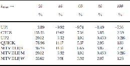
The spatially second-order schemes UP2 and MTVDLF/ M give the best results throughout (except at kmax = 20, as noted above), and further, the results of the two schemes are identical. Closer inspection shows that this surprising finding does not hold in general, but is due to our particular problem (see Appendix). the errors rb of both schemes are very small, ≤1% for kmax ≥ 60. Even for the third-order scheme QUICK, rb is distinctly greater than for UP2 and MTVDLF/M at all resolutions. As for the TVD schemes, application of the less diffusive limiters (MTVDLF/S, MTVDLF/W) reduces the accuracy, so that some numerical diffusion is evidently desirable.
The CTCS scheme is particularly bad for small numbers of gridpoints, kmax = 20, 40. This is because it tends to produce some oscillations over the whole spatial domain, which may even lead to unstable integrations. These oscillations become evident in Figure 3, which shows the relative errors of the computed age profiles as functions of z for kmax = 20, 100 (schemes MTVDLF/S,W not considered). An attempt may be made to minimize this problem by adjusting the frequency of FTCS steps (section 3.3), but nevertheless the CTCS scheme cannot be recommended due to this susceptibility to instabilities.
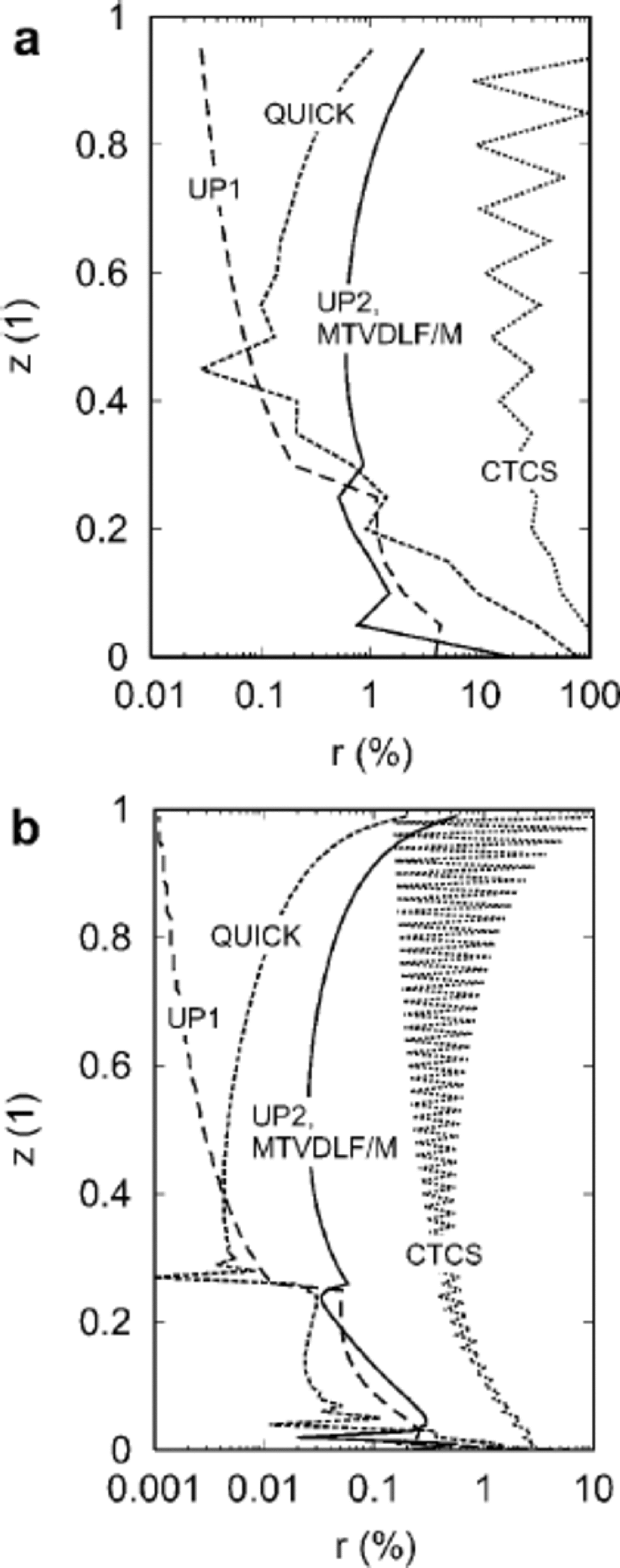
Fig. 3 Relative errors r of computed ages (see Equation (24)) for (a)> kmax = 20 and (b) kmax = 100.
A comparison of the relative errors of UP1, UP2, MTVDLF/M and QUICK over the whole column is instructive (see Fig. 3). for UP1 the error is smallest close to the surface and increases essentially monotonically toward the base. By contrast, for UP2, MTVDLF/M and QUICK the errors are somewhat larger close to the surface, reach a minimum at approximately half the depth and increase again further down. This is probably because UP2, MTVDLF/M and QUICK use central interpolation like CTCS for the age ![]() see Equations (32)2 and (34)2), so that the near-surface error resembles that of CTCS. the errors of UP1 and QUICK are smaller than those of UP2 and MTVDLF/M for
see Equations (32)2 and (34)2), so that the near-surface error resembles that of CTCS. the errors of UP1 and QUICK are smaller than those of UP2 and MTVDLF/M for ![]() (small age gradients), whereas for z < z* (large age gradients) UP2 and MTVDLF/M perform better. Nevertheless, except for the very basal gridpoint at z = 0 (see above discussion of the basal error) the simplest UP1 scheme yields results comparable to those of UP2 and MTVDLF/M for high and low resolutions.
(small age gradients), whereas for z < z* (large age gradients) UP2 and MTVDLF/M perform better. Nevertheless, except for the very basal gridpoint at z = 0 (see above discussion of the basal error) the simplest UP1 scheme yields results comparable to those of UP2 and MTVDLF/M for high and low resolutions.
At the transition point ![]() where the vertical velocity is discontinuous in the second and the age in the third z derivative, the errors of UP1, UP2, MTVDLF/M and QUICK show some jumps, naturally more pronounced for high resolution. Further, some oscillations appear for high resolution close to the base. Generally, among those schemes the most artificial structure is introduced to the age profile by QUICK due to its high spatial order.
where the vertical velocity is discontinuous in the second and the age in the third z derivative, the errors of UP1, UP2, MTVDLF/M and QUICK show some jumps, naturally more pronounced for high resolution. Further, some oscillations appear for high resolution close to the base. Generally, among those schemes the most artificial structure is introduced to the age profile by QUICK due to its high spatial order.
It is worth noting that in other similar models, different schemes are favoured. Reference Wang, Straughan, Greve, Ehrentraut and WangWang and Hutter (2001) investigate the one-dimensional problem of a discontinuity (Heaviside step) of some field quantity which travels with constant velocity c in direction x in an infinitely extended system governed by the advective wave equation ![]() Apart from the missing source term, the constant velocity and the missing boundaries, this model equation is equivalent to our age equation (15). However, the moving discontinuity poses a challenge to numerical schemes that is not present for our continuous age profile. Reference Wang, Straughan, Greve, Ehrentraut and WangWang and Hutter (2001) show that numerical diffusion in the UP1 scheme largely smears out the discontinuity, and CTCS, UP2 and QUICK produce some numerical oscillations in the vicinity of the discontinuity. Best reproduction is achieved by the MTVDLF schemes; however, in contrast to our problem the less diffusive limiters (MTVDLF/S, MTVDLF/W) are favourable because they best preserve the shape of the Heaviside step.
Apart from the missing source term, the constant velocity and the missing boundaries, this model equation is equivalent to our age equation (15). However, the moving discontinuity poses a challenge to numerical schemes that is not present for our continuous age profile. Reference Wang, Straughan, Greve, Ehrentraut and WangWang and Hutter (2001) show that numerical diffusion in the UP1 scheme largely smears out the discontinuity, and CTCS, UP2 and QUICK produce some numerical oscillations in the vicinity of the discontinuity. Best reproduction is achieved by the MTVDLF schemes; however, in contrast to our problem the less diffusive limiters (MTVDLF/S, MTVDLF/W) are favourable because they best preserve the shape of the Heaviside step.
To conclude, our tests show clearly that second-order upstreaming (UP2), modified TVD Lax–Friedrichs (MTVDLF/M) solution techniques and, with limitations of the accuracy directly at the base for higher resolutions, even first-order upstreaming (UP1) yield the best results for typical age profiles in ice sheets (here approximated by a one-dimensional model problem). UP1 and UP2 are less expensive computationally, but spatial discontinuities of the age field (which are not included in our model problem) will either be smeared out (UP1) or will be accompanied by artificial oscillations (UP2). MTVDLF/M has the potential to reproduce such jumps more accurately at the cost of more computing time.
Generalization of the methods presented in section 3 to three-dimensional time-dependent situations described by Equation (3) is straightforward and will be carried out in the near future within the ice-sheet model SICOPOLIS. the applicability to such problems was successfully demonstrated by Reference Wang, Straughan, Greve, Ehrentraut and WangWang (2001) in the context of wind-induced circulations in lakes, where three-dimensional advection occurs in the evolution equations for the flow velocity and the temperature field.
Acknowledgements
The very thorough and constructive reviews of C. L. Hulbe and an anonymous referee are gratefully acknowledged. We also thank K. Hutter for reading and correcting the original manuscript. the scientific editor was T.H. Jacka.
Appendix
Equivalence Between MTVDLF/M AND UP2
The equivalence between the two schemes MTVDLF/M and UP2 for our particular problem can be proved in the following manner. for the whole spatial domain 0 ≤ z ≤ 1, the analytical steady-state solution of the age equation (15) has the properties
(see Fig. 1). Provided the numerical solution at time tn is sufficiently close to the analytical steady state so that these relations also hold for the numerical solution, then, due to (A1)3,
and with (A1)2,
so that the slope limiter (Equations (36) and (37)) computed with Minmod is
Thus, from Equation (42),
When this result and condition (A1)1 in the form |vz| = –vz are inserted into the MTVDLF/M scheme (Equation (45)), it reduces to the UP2 scheme (Equation (32)) for all grid-points k = 0 . . . kmax.
The equivalence of MTVDLF/Mand UP2 can be similarly shown for the cases
For case (A6) the proof is analogous to (A1), whereas for (A7) and (A8),
so that the slope limiter is
which is (except for k = 0) the upstream direction for positive velocities vz.


