


1. Introduction
Over the past few decades, Arctic sea-ice cover has decreased dramatically (Reference Comiso, Parkinson, Gersten and StockComiso and others, 2008). In September 2007 it reached a record minimum of 37% less than the climatological average over 1979–2007. the extent of summer Arctic sea-ice cover is a sensitive indicator of climate change, and is also a potential amplifier of climate change through the ice-albedo feedback mechanism, resulting from the contrast between the albedo of sea ice and open water.
Solar radiation is the dominant energy source driving sea-ice melting during the summer. Reference Perovich, Light, Jones, Runciman and NghiemPerovich and others (2007) examined satellite-derived ice concentrations and solar radiation, determined from reanalysis data, to show that decreases in sea-ice extent led to an increase in the amount of solar energy absorbed in the upper ocean, in turn accelerating sea-ice decay through ice-albedo feedback. the disposition of incoming solar radiation within sea ice and the upper ocean is critical to the heat and mass balance of sea ice. the heat balance of the ice–upper-ocean coupled system has been examined by simple ice–ocean coupled models (e.g. Reference SteeleSteele, 1992; Reference Ebert, Schramm and CurryEbert and others, 1995). However, there have been few observational studies examining the ice–upper-ocean coupled system of the Arctic Ocean. Reference Inoue, Kikuchi and PerovichInoue and others (2008) suggested that the relationship between ice concentration and upper ocean temperature is a good indicator for evaluating the heat balance of solar heat input, sea-ice melting, and heat storage in the ocean mixed layer, by observing the ice and ocean from icebreakers. In summer 2007, ice mass-balance observation demonstrated that there was an extraordinarily large amount of bottom melting of ice in the Canada Basin and that solar heating of the upper ocean was the primary heat source (Reference Perovich, Jones and LightPerovich and others, 2008). While much of the solar radiation transmitted to the ocean is through open water, a substantial portion is also transmitted through ponded ice. Reference PerovichPerovich (2005) and Reference Inoue, Kikuchi and PerovichInoue and others (2008) suggested that there was an effect of solar radiation transmittance through ponded ice on sea-ice melting, based on the year-long drift of the ice station SHEBA (Surface Heat Budget of the Arctic Ocean) in 1998 and on trans-Arctic cruises conducted by the US Coast Guard Cutter (USCGC) Healy in 2005. Further reductions in summer sea-ice extent have continued since these observations were made. Additionally, thick and old ice has decreased rapidly (Reference Maslanik, Fowler, Drobot and ZwallyMaslanik and others, 2007). Transmitted solar radiation through the ice may be enhanced because of decreasing average sea-ice thickness in the Arctic Ocean. To understand the sea-ice melting process under recent reduced-ice conditions, additional in situ ice and ocean observations are needed.
We observed sea-ice cover and upper ocean conditions from icebreakers in the Arctic Ocean (Fig. 1). From August to September 2006 and from July to August 2007, the Canadian Coast Guard Ship (CCGS) Louis S. St-Laurent operated in the Canada Basin. From July to September 2007, the Research Vessel (R/V) Polarstern operated in the eastern Arctic Ocean. the purpose of this study was to describe sea-ice melting processes, based on ice and ocean conditions data, obtained during the summer from icebreakers in the Arctic, and to compare these results with those of a simple ice–upper-ocean coupled model.

Fig. 1. Time series of sea-ice concentration in the Arctic Ocean on (a) 1 August 2006, (b) 1 September 2006, (c) 1 August 2007, (d) 1 September 2007, (e) 1 August 2008 and (f) 1 September 2008, deduced from Advanced Microwave Scanning Radiometer for Earth Observing System (AMSRE) data provided by the US National Snow and Ice Data Center (NSIDC). the NASA Team algorithm is used. the cruise tracks are superimposed. Red line in (a) and (b) denotes the cruise tracks of CCGS Louis S. St-Laurent in 2006. Light blue line in (a) and (b) denotes the trajectory of ITP3/IMB2005B from July to August in 2006. Red line in (c) and (d) denotes the cruise tracks of CCGS Louis S. St-Laurent in 2007. Yellow line in (c) and (d) denotes the FYI region during cruise CCGS Louis S. St-Laurent in 2007. Green line in (c) and (d) denotes the cruise track of R/V Polarstern in 2007. Light blue line in (c) and (d) denotes the trajectory of ITP6/IMB2006C from July to August in 2007. Light blue and green lines in (e) and (f) denote the trajectories of ITP13/IMB2007E and ITP18/IMB2007F from July to August in 2008. Thick lines in (a), (c) and (e) ((b), (d) and (f)) indicate the ship position in August (September).
2. Observations
The CCGS Louis S. St-Laurent operated in the Canada Basin from the beginning of August until mid-September 2006 and from the end of July until the end of August 2007 (hereafter, we call these cruises LSSL2006 and LSSL2007, respectively). From the end of July until the end of September 2007, the German R/V Polarstern operated in the eastern Arctic Ocean (hereafter PS2007). the cruise routes of LSSL2006, LSSL2007 and PS2007 are shown in Figure 1, superimposed on satellite images of sea-ice concentrations.
Temperature and salinity data obtained from conductivity–temperature–depth (CTD) units and expendable CTD (XCTD) were used in this study. Visual observations of sea-ice cover were made, according to the methods of Reference Worby, Allison and DiritaWorby and others (1999), from the bridge while the ship was moving through the ice (Fig. 2). For each visual observation, we estimated ice concentration, ice type and ice thickness. Time intervals for each parameter are listed in Table 1. In this study, we used data on the percentages of open water, ponds, ice, and ice type and thickness.

Fig. 2. Photographs of the ice cover taken from the bridge of LSSL2007 at (a) 76˚ N, 150˚W and (b) 77˚ N, 135˚ W.
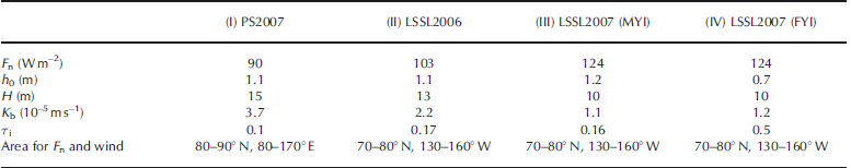
Table 1. Time interval of visual ice observation during PS2007, LSSL2006 and LSSL2007. Dashes indicate the parameter was not observed

In addition to the ship-based data, ice and ocean data obtained from ice mass-balance buoys (IMBs) and ice-tethered profilers (ITPs) were used. Observations of the ice surface and bottom melt were made using autonomous IMBs (D.K. Perovich and others, http://imb.crrel.usace.army.mil)that drifted with the ice pack. ITPs, which collected temperature and salinity profiles beneath the ice to 800m (Reference Krishfield, Toole, Proshutinsky and TimmermansKrishfield and others, 2008), were also deployed. Here, ocean and ice data were examined using ITPs (ITP3, ITP6, ITP13, ITP18) and co-located IMBs (IMB2005B, IMB2006C, IMB2007E, IMB2007F) in the Canada Basin during the melting seasons in 2006, 2007 and 2008 (Fig. 1).
3. Ice and Ocean Conditions
Figure 1 shows the time series of sea-ice concentrations during summer in 2006, 2007 and 2008. Summer sea-ice extent has decreased significantly since the late 1990s. Sea-ice extent in 2006, 2007 and 2008 has shrunk compared with that existing before the 2000s. In particular, in September 2007 the extent of Arctic sea-ice cover reached a record minimum, which was 37% less than the climatological average over the period since September 1979 (Reference Maslanik, Fowler, Drobot and ZwallyMaslanik and others, 2007; Reference Comiso, Parkinson, Gersten and StockComiso and others, 2008). the retreat was particularly pronounced on the Pacific side of the Arctic Ocean. In most of the observational area of LSSL2007, the sea ice had completely melted by mid-September. In September 2006 and 2008, the sea ice did not retreat as much as it did in 2007. Interestingly, a polynya appeared above Northwind Ridge (~76˚ N, 160˚ W) in 2006.
Figures 3–5 show the distribution of the observed ice and ocean characteristics along the cruise routes of PS2007, LSSL2006 and LSSL2007, respectively. Temperature and salinity were approximately uniform from near the surface to depths of 10–25m (data not shown). Thus, we used the average temperature and salinity from 8 to 12m as the surface mixed-layer temperature and salinity. Temperature above the freezing point of local sea water (ΔT) is a good indicator of how much the upper ocean is heated by solar radiation, particularly in areas where salinity is not horizontally uniform.

Fig. 3. Ice and ocean observational data from PS2007 cruise. (a) Solid and dashed curves indicate latitude and longitude of ship position corresponding to the cruise track. Solid line indicates the analysis areas in Figure 6a. (b–d) Distribution of (b) temperature and salinity between 8 and 12 m derived from the CTD and XCTD data (filled cricles: temperature; open circles: salinity), (c) ice concentration derived from ice-watch data (dark grey: open water; light grey: melt pond; white: sea ice) and ice concentration deduced from AMSRE data (solid curve) and (d) ice thickness obtained by the ice watch.

Fig. 4. Ice and ocean observational data from LSSL2006 cruise. (a) and (b) correspond to Figure 3a and b, respectively. Solid line in (a) indicates the analysis areas in Figure 6b. (c) Distribution of ice concentration derived from ice-watch data (dark grey: open water; white: sea ice) and ice concentration deduced from AMSRE data (solid curve). Melt pond fraction and ice thickness observation were not carried out.

Fig. 5. Ice and ocean observational data from LSSL2007 cruise. (a), (b) and (d) correspond to Figure 3a, b and d, respectively. (c, e) Distribution of (c) ice concentration derived from ice-watch data (dark grey: open water; white: sea ice; light gray dots: melt pond fraction) and ice concentration deduced from AMSRE data (solid line) and (e) fractions of multi-year ice (MYI) and first-year ice (FYI) from ice watch (filled circles: MYI; open circle: FYI). Sums of the fractions of MYI and FYI are equal to A i. Black and gray lines in (a) indicate the analysis areas in Figure 6c and d.
The temperature was typically above freezing even in regions that were almost completely ice-covered (>90% cover), as shown in Figure 3–5. During LSSL2007, ΔT was very high in the open-water and marginal-ice regions of the southern Canada Basin. We discuss this in more detail in sections 4 and 5. Melt ponds covered 27% and 31% of the sea-ice area during PS2007 and LSSL2007, respectively. the average ice thicknesses during PS2007 and LSSL2007 were 0.9 and 1.0 m, respectively. Average ice thickness in the central Arctic (north of 85˚ N) was 0.8 m in 2007 and 1.9 m in 2005 from trans-Arctic observations (Reference PerovichPerovich and others, 2009), suggesting decreasing ice thickness from 2005 to 2007. Melt pond fraction and ice thickness observations were not carried out during LSSL2006.
4. Relationships Between Ice Concentration and Water Temperature
The relationship between ice concentration and temperature is a consequence of heat balance in the ice–upper-ocean coupled system, maintained by solar radiation, sea-ice melting, and heat storage in the ocean mixed layer (Reference Ohshima, Yoshida, Wakatsuchi, Endoh and FukuchiOhshima and others, 1998; Reference Inoue, Kikuchi and PerovichInoue and others, 2008). Here we describe the relationships between ice concentrations observed by on-board ice watch and upper ocean temperatures obtained by CTD and XCTD observation. Because local heat balances in the ice–upper-ocean system hold over 20–30km spatial scales (Reference Ohshima, Yoshida, Wakatsuchi, Endoh and FukuchiOhshima and others, 1998; Reference Nihashi, Ohshima, Jeffries and KawamuraNihashi and others, 2005), ice and ocean data in areas where the ice concentration was >50% were averaged to a 25 km spatial running mean. We refer to PS2007 and LSSL2006 as cases I and II, respectively. We divided the stations of LSSL2007 into two areas, because sea-ice thickness and the relationship between ice concentration and temperature in the southern Canada Basin were very different from those in the northern Canada Basin. We refer to the thick multi-year ice (MYI) region (ice thickness h = 1.2 m) and the thin first-year ice (FYI) region (h = 0.7 m) as cases III and IV, respectively. During LSSL2007, ΔT was very high in the open-water and marginal-ice regions of the southern Canada Basin. Additionally, the ΔT from 6 to 11 August in the southern Canada Basin along 150˚\W below 78˚N was higher than that from 11 to 19 August in the northern Canada Basin above 78˚ N, although the ice concentration remained high (80–90%) from 6 to 19 August. In the former region, ice thickness was relatively low (<1 m) and the fraction of MYI was almost zero (see Fig. 2a). As these stations are 100–1000km from the ice margin, heat advection from open-water areas is not a reasonable explanation.
Figure 6 shows the ice-concentration (A i)–ΔT plots (hereinafter CT plots) during August for cases I–IV. In all cases, ΔT increased as the ice concentration decreased, consistent with results obtained from Antarctic cruises off Syowa station (Reference Ohshima, Yoshida, Wakatsuchi, Endoh and FukuchiOhshima and others, 1998) and in the Ross Sea (Reference Nihashi, Ohshima, Jeffries and KawamuraNihashi and others, 2005), and Arctic cruises in the Canada Basin (Reference Inoue, Kikuchi and PerovichInoue and others, 2008). This indicates that as ice concentration decreases, ΔT increases due to the greater absorption of solar radiation into open water (ice-albedo feedback). Correlation coefficients between ΔT and 1/A i for cases I–III were above the 99% confidence level for significance. If heat advection from open water outside the ice edge, vertical heat flux from below the mixed layer, and transmittance of solar radiation through the ice are neglected, ΔT should approach 0˚C towards 100% ice concentration on a CT plot (Reference Ohshima, Yoshida, Wakatsuchi, Endoh and FukuchiOhshima and others, 1998; Reference Nihashi, Ohshima, Jeffries and KawamuraNihashi and others, 2005; Reference Inoue, Kikuchi and PerovichInoue and others, 2008). However, ΔT was above zero even in almost completely ice-covered regions (e.g. ice concentrations of >90%). Heat advection from open-water areas is not a reasonable explanation for this increased ΔT (hereinafter ΔT-gain), because the ΔTwas above zero even 100–1000km from the ice edge. Vertical heat flux from below the mixed layer can also be neglected due to strong stratification during the Arctic summer. Thus, transmittance of solar radiation through ponded ice apparently affected ΔT-gain in largely ice-covered regions, consistent with the results of Reference Inoue, Kikuchi and PerovichInoue and others (2008).

Fig. 6. Scatter plots of the ice concentration versus temperature above the freezing point (ΔT) from (a) case I, (b) case II, (c) case III and (d) case IV. Ice concentration derived from on-board ice-watch data and ΔT calculated from the CTD and XCTD data are spatially averaged using a 25 km running mean. the dashed curves are regression curves (linear with respect to 1/A i) based on the observations. R and RMSE indicate the correlation coefficient and root-mean-square error, respectively. the solid curve is the same regression curve after subtracting the quantity (ΔT-gain A i=100%A i), which we take as the warming caused by transmission of solar radiation through the ponded ice.
According to the analytic solution obtained by Reference Ohshima, Yoshida, Wakatsuchi, Endoh and FukuchiOhshima and others (1998), ΔT is inversely proportional to A i. In fact, CT plots from Reference Ohshima, Yoshida, Wakatsuchi, Endoh and FukuchiOhshima and others (1998), Reference Nihashi, Ohshima, Jeffries and KawamuraNihashi and others (2005) and Reference Inoue, Kikuchi and PerovichInoue and others (2008) show inverse proportionality. Thus, we applied simple regression lines (ΔT = α/A i + β), similar to Reference Inoue, Kikuchi and PerovichInoue and others (2008). the dashed curves in Figure 6 are regression curves based on the observations for each area. the total ΔT-gain is the sum of the contributions of heat from open water and ponded ice. ΔT-gain where the ice concentration is 100% (ΔT-gain A i=100%) should be ΔT-gain only resulting from heat transmittance through ponded ice (ΔT i). Therefore, ΔT-gain resulting from heat input through open water (ΔT o) can be obtained by subtracting the ΔT-gainA i=100%, weighted by A i, from the total ΔT-gain. We note that the discussion here assumes that pond fraction and transmittance of ponded area does not change as A i decreases. the solid curves in Figure 6 are adjusted regression lines for ΔT o (ΔT-gain – ΔT-gainA i=100% A i). the area enclosed between these two curves indicates the ΔT i induced by A i. In a specific example, to gain 0.068˚C of ΔT when 90% of the area was covered by ponded ice, total ΔT-gain was partitioned into ΔT o = 0.03˚C and ΔT i = 0.038˚C in Figure 6a. Although the contribution of ΔT o was the dominant heat source over most of the area, the role of ΔT i was considerable beneath largely ice-covered areas. the contribution of ΔT i to total ΔT-gain was greater than that of ΔT o where the ice concentration was more than 88%, 82%, 83% and 65%, for cases I, II, III and IV, respectively.
Even at the same ice concentrations, ΔT-gains were different between cases I, II, III and IV (Fig. 6). the ΔT i was anomalously high in case IV (LSSL2007 FYI region). As these stations were far from the north of the ice margin (100– 1000 km), heat input due to transmitted solar radiation through the ice rather than horizontal heat advection from open-water areas is a reasonable explanation for this ΔT i. We examine ΔT-gain more closely in section 5, using a simple ice–ocean coupled model.
From PS2007, only data from the 90˚ E section are shown in Figure 6. Sections along 34˚ E and 60˚ E, in the Nansen Basin, also showed negative correlations in the CT plots, although ΔT-gain was higher than in case I. A possible explanation for this might be differences in solar radiation because of the timing of observations and/or the horizontal heat advection of Atlantic water from open water. As the number of stations in this area was so small, we did not include them in this study.
5. Simple Models to Evaluate Heat Balance of Ice–Upper-Ocean Coupled System
In this section, we develop a simple model to examine the observed ice concentration and temperature relations, which is a consequence of the heat balance in the ice– upper-ocean coupled system in the Arctic melting season.
5.1. A model without transmitted solar radiation through the ponded ice
5.1.1. Model description
As heat input into the ice–upper-ocean system mainly occurs in open water when the ice concentration is relatively low, we began by examining the observed CT plot using a simple ice–upper-ocean coupled model in which sea-ice bottom and lateral melting are caused only by the heat input through open water (as proposed by Ohshima and Reference Nihashi, Ohshima, Jeffries and KawamuraNihashi (2005) and Reference Inoue, Kikuchi and PerovichInoue and others (2008)). As shown in section 4, we separately evaluated the surface water heating caused by heat input through open-water areas (ΔT o) and through ponded ice areas (ΔT i), using simple regression curves applied to observed CT plots (Fig. 6). Here we briefly describe the model, schematically shown in Figure 7a. the upper ocean is represented simply by a mixed layer of thickness H with a uniform temperature, T, and salinity, S. Heat and water exchange with the ocean below the mixed layer are also assumed to be zero due to the strong stratification during the Arctic summer. the net heat flux to the ocean over the ice-covered area, A i, is assumed to be zero; thus, the surface net heat flux would only be supplied in the open-water area, 1 – A i. If sea-ice melting is caused by this heat input, the heat balance of the upper ocean can be given by

Fig. 7. A schematic illustration of the coupled ice–ocean model. A i is ice concentration, so 1 – A i is the open-water fraction. h is ice thickness. the upper ocean is simply represented by one layer of thickness H with a uniform temperature, T, and salinity, S. (a) Incident solar flux at the surface, F n, is supplied only over the open-water area. (b) Transmitted solar radiation through the ponded ice area is included as well as heat flux into the open-water area.
where F n is the incident solar flux at the surface, c w = 3990 J kg–1 K–1 is the heat capacity of sea water, ρ w = 1026 kgm–3 and ρ i = 900 kgm–3 are the densities of sea water and sea ice, respectively, L f is the latent heat of fusion for sea ice and t is time. We used a fixed value of L f = 0.316 MJ kg–1, corresponding to a MYI salinity of 2 psu (Reference Eicken, Lensu, Tucker, Gow and SalmelaEicken and others, 1995). the ice thickness, h, is defined as the average thickness, and α o = 0.06 is the surface albedo of open water.
We assume that sea ice melts at the bottom and lateral faces at a rate proportional to the difference between the water temperature and the freezing point (i.e. ΔT). We implicitly assume that the open water is well mixed with the water just beneath the ice. Bottom melting is parameterized as
where K b is the bulk heat transfer coefficient between ice and ocean. Lateral melting is parameterized in a similar way to Reference HiblerHibler (1979), as
In this equation, h* is defined as an effective sea-ice thickness averaged over each of the gridcells, including the open-water fraction. Thus, h* can be regarded as the total ice volume per unit area. Note that the actual average ice thickness is h = h* /A i in this model.
Using this model, we discuss the relationships between the ice fraction and the temperature above the freezing point. on the basis of in situ observations from the icebreakers, the surface mixed layer thickness, H, and initial sea-ice thickness, h 0, were set to the values listed in Table 2. the incident solar flux at the surface, F n, was set to one-third of the shortwave radiation at the top of the atmosphere for each area using Reference KeyKey’s (2001) radiative transfer model, as a follow-on to the results of Reference Inoue, Kikuchi, Perovich and MorisonInoue and others (2005, Reference Inoue, Kikuchi and Perovich2008). the F n averaged over the period from 5 days before observations began until the end of the observation period for the study area noted in Table 2 was used for model calculations, because 10–15 days corresponds to the convergence timescales of the model (Reference Ohshima, Yoshida, Wakatsuchi, Endoh and FukuchiOhshima and others, 1998; Ohshima and Reference Nihashi, Ohshima, Jeffries and KawamuraNihashi, 2005; Reference Inoue, Kikuchi and PerovichInoue and others, 2008). the model values of F n are listed in Table 2.
Table 2. Value of each parameter for simple ice–ocean model for PS2007, LSSL2006 and LSSL2007 (both MYI and FYI). F n is incident solar flux at the surface, h 0 is initial ice thickness, H is mixed-layer thickness, K b is heat transfer coefficient between ice and ocean, and τ i is solar radiation transmittance through ponded ice area. F n and wind speed data used in Figure 12 are averaged in the bottom row
5.1.2. Results
The CT relationship converges asymptotically with a timescale of 10 days regardless of the initial conditions of A i and ΔT (Reference Ohshima, Yoshida, Wakatsuchi, Endoh and FukuchiOhshima and others, 1998; Ohshima and Reference Nihashi, Ohshima, Jeffries and KawamuraNihashi, 2005; Reference Inoue, Kikuchi and PerovichInoue and others, 2008). ΔT is zero under completely ice-covered areas, because solar radiation transmittance through the ice is not treated in this model. Therefore, the modeled ΔT-gain is comparable to the analyzed ΔT o calculated from the linear regression curve shown by a solid curve in Figure 6. the characteristics of the convergent curves are determined by parameters, F n, K b, h and H. Because h and H are observable parameters and F n can be obtained as described above, K b is the least-known parameter. the modeled CT relationship can be used to estimate the bulk heat transfer coefficient between ice and ocean, K b, by least-squares fitting the analyzed ΔT o. the blue curves with the values of K b noted in Figure 8 provided the best fit to the observed CT plots for cases I–IV. In section 5.1.1 we show that these derived values of K b seems to be physically reasonable. Using estimated values of K b, the modeled CT relationships agreed with the analyzed A i–ΔT o relationships (Fig. 8), suggesting that the model can approximately describe the heat balance of the ice–upper-ocean system that includes only heat input through open water.

Fig. 8. Blue and red solid circles are model results without and with effect of solar radiation transmittance through the ponded ice area after 15 days of time integration. Convergent curves are linearly extrapolated toward 100% ice concentration with respect to 1/A i. Open blue and red circles indicate the extrapolated values. Dashed blue curves show the results with F n changed by ±15Wm–2. Dashed red curves show the results with ± i changed by ±0.05 (cases I, II and III) or ±0.15 (case IV). the solid and dashed black curves are the same as shown in Figure 6.
Here we briefly examine the dependence of the CT plots on the controlling factors, F n, K b, h and H. In a test case, F n, K b and H were set to 120Wm–2, 2.0×10⁻⁵ms–1 and 13 m, corresponding to typical summertime values in the Arctic. Initial ice thickness is set to 1.2 m. To examine the sensitivity of the calculated CT curve to variations in F n, K b, h and H, cases with these parameters halved and doubled are shown in Figure 9. In regions with relatively high ice cover, the

Fig. 9. Relationship between ice concentration and upper-ocean temperature above freezing, derived from the ice–ocean coupled model illustrated in Figure 7a. the solid black curve shows the base case with initial ice thickness set to 1.2 m, F n set to 120Wm–2, and K b set to 2.0×10⁻⁵ms–1. Red, blue, yellow and green thick (thin) dotted curves indicate cases with F n, K b, h and H, respectively, doubled (halved) from the base case.
modeled curves are most sensitive to F n and K b. To examine the sensitivity of CT plots for cases I–IV to changes in F n, the results with F n changes by ±15m–2, approximately the variation of F n among our cases, are also plotted in Figure 8. In regions with relatively high (>70%) ice cover, the resulting differences in ΔT were <0.1˚C. This is much smaller than the observed ΔT difference among cases I–IV, which was caused by both F n and K b differences. Thus, the observed ΔT difference is primarily due to K b.
Figure 10 shows the ratio of heat used for ice melt to heat input into open water for cases I–IV in the model. the heat ratio also converges asymptotically, with a timescale of 10 days (Ohshima and Reference Nihashi, Ohshima, Jeffries and KawamuraNihashi, 2005). This indicates that the distribution of upper-ocean heat between sea-ice melt and upper-ocean heating can be determined by ice concentration. In regions of relatively high (>70%) ice cover, the total heat input to open water is distributed 80–95% to ice melting and 5–20% to upper-ocean heating during the Arctic summer. Reference Toole, Timmermans, Perovich, Krishfield, Proshutinsky and Richter-MengeToole and others (2010) proposed that 76% of total heat into open water went to bottom melt, based on the result from a one-dimensional mixed-layer model, which is consistent with the observation by ITP and IMB from June to early September 2007. Over that observational period, ice concentration averaged ~60%. Their result supports our estimation of heat balance between ice melting and ocean heating.

Fig. 10. Ratio of the heat used for ice melt to the heat input through open water as a function of ice concentration, derived from the ice– ocean coupled model illustrated in Figure 7a. Thick dotted, thin dotted, thick solid and thin solid curves denote the results with the parameters for cases I, II, III and IV, respectively.
5.1.3. Bulk heat transfer coefficient in the ice–upper-ocean system, Kb
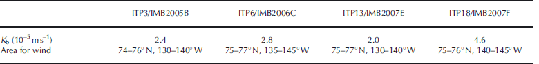
The K b estimated by our model is a bulk heat transfer coefficient in the ice–upper-ocean system. However, Reference McPheeMcPhee (1992) and Reference McPhee, Kikuchi, Morison and StantonMcPhee and others (2003) estimated the heat transfer coefficient using the eddy correlation method in the Arctic Ocean. K b in this study corresponds to Ch ×Uτ in their study (Ch : heat transfer coefficient; Uτ : friction velocity). the estimated K b in Reference McPheeMcPhee (1992) and Reference McPhee, Kikuchi, Morison and StantonMcPhee and others (2003) was 3.1×10⁻⁵ms–1, which is of the same order as that estimated in this study. Based on results from the Antarctic Ocean, Reference Nihashi and OhshimaNihashi and Ohshima (2008) proposed that K b was proportional to the cubed or squared wind speed (friction velocity). Here we examine the relationship between the estimated K b listed in Table 3, and wind speed in the Arctic Ocean.
Table 3. The estimated K b for ITP3/IMB2005B, ITP6/IMB2006C, ITP13/IMB2007E and ITP18/IMB2007F. Wind speed data used in Figure 12 are averaged in the bottom row
K b can also be estimated based on data from ITP and IMB. Equation (4) can be obtained by canceling A i from Equation (2).
We used the ΔT averaged from 8 to 12 m during July and August for each ITP. Rates of bottom melt (dh/dt) were calculated from changes in ice flow depth over that period for each co-located IMB.
Figure 11 shows the relationship between estimated K b and wind speed. the K b values are those estimated in this subsection for our four cases, along with those estimated above from the ITP/IMB data, and one additional
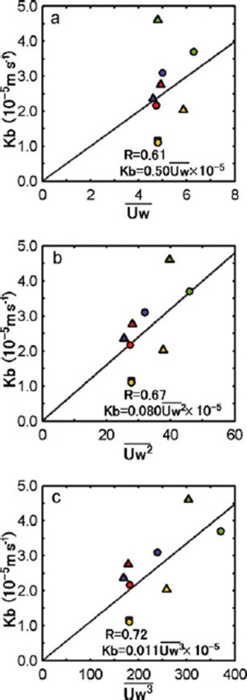
Fig. 11. Scatter plots of the bulk heat transfer coefficient, K
b, versus wind speed. Six-hourly 10m wind speed data from ERA-Interim provided by ECMWF over the period from 5 days before observations began to the end of the observation ![]() for the study area noted in Tables 2 and 3 are used in (a).
for the study area noted in Tables 2 and 3 are used in (a). ![]() and
and ![]() by averaging
by averaging ![]() over that period for each area are used in (b) and (c), respectively. Solid line is a least-squares fittings line. Blue, red, yellow and green dots indicate results from a cruise on the Healy in 2005 (Reference Inoue, Kikuchi and PerovichInoue and others, 2008), cases I, II and III, respectively. Yellow squares indicate results from case IV. Blue, red, yellow and green triangles indicate results from ITP3/IMB2005B, ITP6/ IMB2006C, ITP13/IMB2007E and ITP18/IMB2007F, respectively.
over that period for each area are used in (b) and (c), respectively. Solid line is a least-squares fittings line. Blue, red, yellow and green dots indicate results from a cruise on the Healy in 2005 (Reference Inoue, Kikuchi and PerovichInoue and others, 2008), cases I, II and III, respectively. Yellow squares indicate results from case IV. Blue, red, yellow and green triangles indicate results from ITP3/IMB2005B, ITP6/ IMB2006C, ITP13/IMB2007E and ITP18/IMB2007F, respectively.
estimate from Reference Inoue, Kikuchi and PerovichInoue and others (2008). the mean wind speed ![]() was calculated from 6 hourly, 10m wind (U
w) from the European Centre for Medium-Range Weather Forecasts (ECMWF) Interim Re-analysis (ERA-Interim) over the areas given in Tables 2 and 3, for the period from 5 days before observations began to the end of the observation period. the quantities
was calculated from 6 hourly, 10m wind (U
w) from the European Centre for Medium-Range Weather Forecasts (ECMWF) Interim Re-analysis (ERA-Interim) over the areas given in Tables 2 and 3, for the period from 5 days before observations began to the end of the observation period. the quantities ![]() and
and ![]() are the mean of
are the mean of ![]() and
and ![]() over the same area and time periods. K
b and surface wind speed are positively correlated, consistent with the results from the Antarctic Ocean reported by Reference Nihashi and OhshimaNihashi and Ohshima (2008). K
b is more likely to be proportional to
over the same area and time periods. K
b and surface wind speed are positively correlated, consistent with the results from the Antarctic Ocean reported by Reference Nihashi and OhshimaNihashi and Ohshima (2008). K
b is more likely to be proportional to ![]() and
and ![]() rather than having a linear relationship with
rather than having a linear relationship with ![]() Each of these correlation coefficients is significant at a level of 95%. These results indicate that upper-ocean heat can be used more for ice melting as wind speed increases if other parameters (F
n, H and h) are constant. Unfortunately, only nine data points were obtained to describe the K
b–surface-wind-speed relationship (Fig. 11), so more observational evidence is needed for further discussion. However, it seems that our derived K
b values for cases I–IV are at least realistic.
Each of these correlation coefficients is significant at a level of 95%. These results indicate that upper-ocean heat can be used more for ice melting as wind speed increases if other parameters (F
n, H and h) are constant. Unfortunately, only nine data points were obtained to describe the K
b–surface-wind-speed relationship (Fig. 11), so more observational evidence is needed for further discussion. However, it seems that our derived K
b values for cases I–IV are at least realistic.
5.2. A model with transmitted solar radiation through ponded ice
5.2.1. Model description
In areas of high ice cover, heat input due to solar radiation through the ponded ice area is also effective in heating the upper ocean, as described in section 4. the model that includes this input is schematically shown in Figure 7b. We examined the effect of transmitted solar radiation through ponded ice on the sea-ice melting process by including additional terms related to these parameters in Equation (1), as proposed by Reference Inoue, Kikuchi and PerovichInoue and others (2008):
where τ o=1–α o = 0.94 and τ i are the transmittance of open water and ponded ice, respectively, and A o is the area fraction of open water. the model does not separately treat transmission through the ponds, but rather accounts for a combined transmission through the ponds and bare ice. the initial conditions are the same as in the previous model (section 5.1).
With this version of the model, the modeled ΔT is greater than 0, even for A i = 1, due to transmitted solar radiation through the ponded ice. the modeled CT relationship can be used to estimate solar radiation transmittance through the ice (τ i) by least-squares fitting the observed CT plots. Curves with the values of τ i noted in Figure 8 provide the best fit to the observed CT plots. In the FYI region (case IV), the estimated τ i was much larger than in the MYI region (cases I, II and III).
5.2.2. Results
The model approximately describes the heat balance of the ice–upper-ocean system that includes heat input through ponded ice, as well as directly into open water (red curves in Fig. 8). Our results indicate that solar radiation transmittance through the ice is highly dependent on sea-ice thickness. the anomalously high ΔT in case IV can be explained by the large solar radiation transmittance through the ponded thin first-year ice. A possible explanation for the τ i differences among the MYI regions of cases I, II and III is the melting stage of sea ice (i.e. fraction and depth of melt ponds).
Reference PerovichPerovich (2005) estimated that the heat transmittance through ponded multi-year ice was 0.16 during the melt season, based on the sea-ice observations of a year-long field experiment (SHEBA). Reference Inoue, Kikuchi and PerovichInoue and others (2008) estimated the solar radiation transmittance of melt ponds and multi-year ice as 0.55 and 0.09, respectively, based on sea-ice and ocean observation by USCGC Healy in 2005. Because melt ponds covered 25% of the sea-ice area during that cruise, solar radiation transmittance of ponded ice area is ~0.21 (=(0.55×0.25) + [0.09×(1 – 0.25)], i.e. (τ pond×pond fraction) + [τ ice×(1 – pond fraction)]). These results are consistent with our estimation of transmittance through the ponded MYI region. There was no observation of solar radiation transmittance of thin first-year ice (h~0.7 m). However, transmittance of thinner ice would be larger than that of thick ice, because radiance in ice rapidly decreases with depth as shown by Reference Perovich, Roesler and PegauPerovich and others (1998).
5.3. Effects of transmitted solar radiation through ponded ice on the acceleration of sea-ice melting
Observed higher ΔT is a consequence of solar radiation transmittance through ponded ice, as suggested above. the evolution of ice concentration and ice thickness can be controlled by heat input through the ice as well as from open water. If a time integration is done using Equations (5), (2) and (3), the time evolution of ice concentration and ice thickness is obtained. Figure 12 shows the changes over time of ice thickness and ice concentration for three cases of ice solar radiation transmission. Solar radiation transmittance through the ice, τ i, is set at 0.0, 0.15 and 0.5. Initial ice concentration and ice thickness are set at 97% and 1.2 m, respectively. F n and K b were set at 120Wm–2 and 2.0×10⁻⁵ms–1, corresponding to typical summertime values in the Arctic.

Fig. 12. Time evolution of ice concentration (a) and sea-ice thickness (b) in August calculated from the ice–upper-ocean coupled model. Time integration is done with Equations (5), (2) and (3). Initial ice concentration and ice thickness are set at 97% and 1.2 m, respectively. F n and K b were set at 120Wm–2 and 2.0×10⁻⁵ms–1. Thick dotted curves denote the case without the effect of solar radiation transmittance through the ice (τ i = 0.0). Thin solid and thick solid curves denote the cases with the effect of solar radiation transmittance through the ponded ice, calculated using τ i = 0.15 (corresponding to thick multi-year ice) and τ i = 0.5 (corresponding to thin first-year ice), respectively.
In calculations including solar radiation transmitted through the ice, sea ice decayed rapidly. For thin first-year ice (τ i = 0.5), both ice thickness and ice concentration decreased about three times as much as they did in multi-year ice (τ i = 0.15). In contrast, in calculations without solar radiation transmission through the ice, the ice thickness and ice concentration hardly changed. As noted by Reference Inoue, Kikuchi and PerovichInoue and others (2008), even in MYI regions (τ i = 0.21) the amplification of ice-albedo feedback by transmitted solar radiation through ponded ice is significantly larger than that of warming perturbation caused by doubled CO2 forcing. In thin FYI areas (τ i = 0.5), this ice-albedo feedback is much stronger due to the larger heat input through the ice.
6. Summary and Discussion
Sea-ice melting processes were inferred from in situ sea-ice and ocean condition data obtained during the Arctic research cruises of the CCGS Louis S. St-Laurent and R/V Polarstern in the summers of 2006 and 2007. We examined the relationships between ice concentrations observed by on-board ice watches and temperatures above freezing (ΔT) in the surface mixed layer obtained from CTD and XCTD data, because ice concentration and the ΔT relationship are consequences of the heat balance in the ice–upper-ocean coupled system, which is maintained by solar radiation, sea-ice melting, and heat storage in the ocean mixed layer. Using spatially averaged data (25 km), ice concentration and temperature plots (CT plots) showed negative correlations. This indicates that as ice concentration decreases, the upper ocean becomes warmer from higher absorption of solar radiation, which, in turn, further promotes ice melting (ice-albedo feedback). Additionally, ΔT showed a positive bias when the region was almost completely ice-covered. This indicates that solar radiation transmittance through ponded ice affects upper-ocean warming, which promotes sea-ice melting, particularly in areas of high ice cover. Using simple regression curves applied to the observed CT plots, we separately evaluated the surface water heating caused by heat input through open water and by heat input through ponded ice. Heat input through ice was found to contribute more to ice melting than did heat input through open water when the ice concentration was more than 82–88% in MYI regions and 65% in FYI regions.
We developed a simple model to clarify the observed ice concentration and temperature relationships. the relationships between ice concentration and surface mixed-layer temperature derived from our model are consistent with the observed relationships. By comparing the observed CT plot and the model, the bulk heat transfer coefficient between ice and ocean (K b) and transmitted solar radiation through the ice were estimated. the estimated K b increased with increasing wind speed. This result indicates that more of the total heat input into the upper ocean can be used for ice melting as wind speed increases. Substantial differences in transmission were found between first-year ice (h = 0.7 m) and multi-year ice (h = 1.2 m). Transmitted solar radiation through thin ponded first-year ice was estimated to be approximately three times larger than that through thick ponded multi-year ice. the time evolution of sea-ice decay calculated from the model suggested that solar radiation transmittance through ponded ice is amplified by the ice-albedo feedback mechanism, particularly in thin ice regions.
Over the past few decades Arctic sea-ice cover has decreased dramatically (Reference Comiso, Parkinson, Gersten and StockComiso and others, 2008). Due to the large contrasts in albedo between sea ice (>0.6) and open water (~0.06), an increase in the open-water fraction enhances solar heat input to the upper ocean, which promotes ice melting. This ice-albedo feedback mechanism accelerates sea-ice decay in the Arctic Ocean (Reference Perovich, Light, Jones, Runciman and NghiemPerovich and others, 2007). As well as open-water areas, in regions of high ice cover, ponded areas act as heat sources due to transmitted solar radiation. Recently, the extent of old and thick multi-year ice has been rapidly reduced (Reference Maslanik, Fowler, Drobot and ZwallyMaslanik and others, 2007; Reference Kwok and RothrockKwok and Rothrock, 2009; Reference Kwok, Cunningham, Wensnahan, Zwally and YiKwok and others, 2009). As thin ice increases in the Arctic Ocean, the average solar radiation transmittance by ponded areas during the melting season will also increase, as suggested in this study. Thus, even if the extent of open water does not increase, heat input to the upper ocean will be enhanced and ice melt accelerated in an Arctic with an increasing seasonal ice zone area.
Acknowledgements
We are greatly indebted to the officers and crew of the CCGS Louis S. St-Laurent and R/V Polarstern, and to the scientists and technicians who collected the data. Comments from the scientific editor, S. Hudson, and two anonymous reviewers were very helpful for improving the manuscript. We thank A. Proshutinsky who is a collaborator on the CCGS Louis S. St-Laurent science cruise and supported by US National Science Foundation (NSF) grant No. OPP-0424864. We also thank U. Schauer who is principal investigator on the R/V Polarstern science cruise. We are deeply indebted to S. Nishino and A. Orlich for their help with observation. We acknowledge S. Nihashi for discussion. Support was also provided by the Japan Agency for Marine–Earth Science and Technology (M.I., J.I., K.S., T.K., J.H.), Fisheries and Oceans Canada (S.Z., F.M., E.C.), the NSF (J.H.) and the International Arctic Research Center (J.H.). the ITP data were collected and made available by the Ice-Tethered Profiler Program based at the Woods Hole Oceanographic Institution (http://www.whoi.edu/itp).


