Introduction

Sea ice is an integral component of the Arctic climate system, restricting exchanges of heat, mass and momentum between the ocean and the atmosphere, reflecting most of the solar radiation incident upon it, releasing salt to the underlying ocean during freezing and transporting fresh water Equatorward through sea-ice advection. It is also of vital importance to the ecology of the Arctic, serving as a habitat for organisms living within it, a platform for animals wandering over it and either a help or a hindrance to numerous marine plant and animal species. Hence, changes in the sea-ice cover can have many outreaching effects on other elements of the polar climate and ecological systems. Furthermore, through the interconnectedness of the climate system, major changes in the sea-ice cover could have more far-reaching effects, extending well beyond the polar regions. For instance, changes in the ice transport of cold fresh water southward in the Greenland Sea could impact the deep-water formation in the northern North Atlantic and thereby affect the conveyor-beltcirculation that cycles through much of the global ocean.

Considerable attention has been given recently to decreases in Arctic sea-ice extents detected through analysis of satellite passive-microwave data since late 1978 (e.g. Reference Johannessen, Miles and BjørgoJohannessen and others, 1995; Reference Maslanik, Serreze and BarryMaslanik and others, 1996; Reference Bjørgo, Johannessen and MilesBjørgo and others, 1997; Reference Parkinson, Cavalieri, Gloersen, Zwally and ComisoParkinson and others, 1999). These studies have emphasized decreases examined for the record length as a whole or for annual or seasonal averages. Here we update the annual and seasonal decreases to a 21 year record through the end of 1999, and additionally present time series and trends for each month. Results are given for the Northern Hemisphere as a whole and for each of nine regions, identified in Figure 1. Although a much longer record would be desired (if available), this 21 year period does include El Ninño and La Ninña episodes, positive and negative phases of the North Atlantic Oscillation and the Arctic Oscillation, and major volcanic eruptions of El Chichón, Mexico (28 March–4 April 1982), and Mount Pinatubo, Philippines (15 June 1991). Hence it provides researchers studying those phenomena with a chance to examine effects they may have had on the Arctic sea-ice cover, thereby helping to quantify the respective climate interconnections.

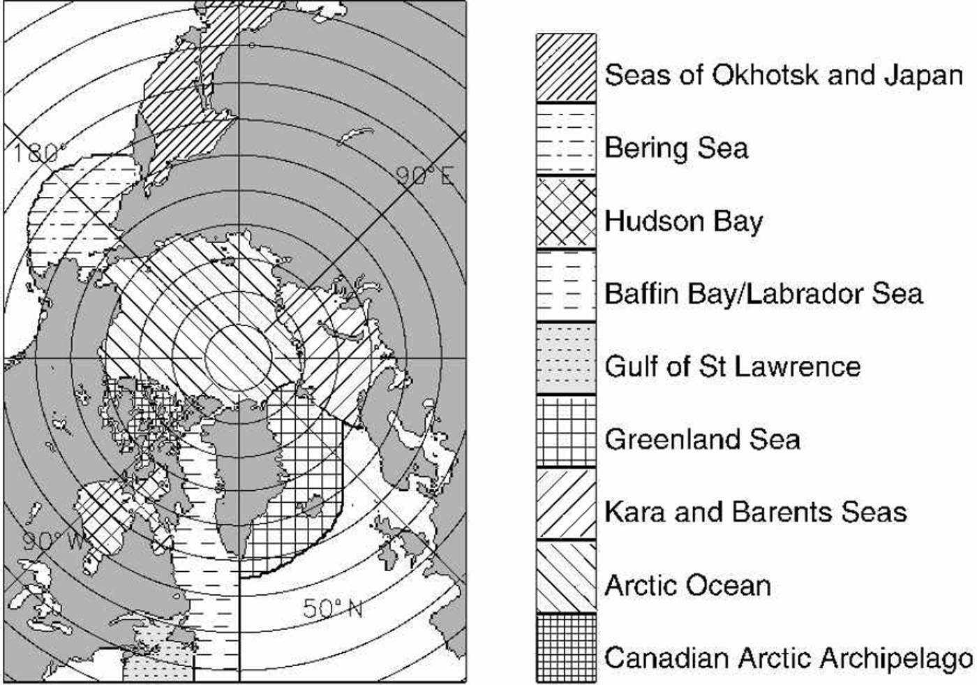
Fig. 1. Identification of the nine regions used in the analysis.

Data And Methodology

The data used in this study are satellite passive-microwave data from the Nimbus 7 Scanning Multichannel Microwave Radiometer (SMMR) and three U.S.Defense Meteorological Satellite Program (DMSP) Special Sensor Microwave/Imagers (SSM/Is). Microwave data are particularly applicable for sea-ice research because the microwave emissions of sea ice and liquid water differ significantly, thereby allowing a ready distinction between ice and water from the satellite microwave data. Complications arise from the diversity of ice surfaces and from melt ponding and snow cover on the ice, but the satellite passive-microwave data still allow a clear depiction of the overall distribution of the ice and thereby allow a calculation of ice extents (areas covered by ice of concentration at least 15%).

The SMMR was operational on an every-other-day basis for most of the period 26 October 1978 to 20 August 1987, and the sequence of SSM/Is has been operational on a daily basis for most of the period since 9 July 1987. The SMMR and SSM/I data have been used to create a consistent dataset of sea-ice concentrations (per cent areal coverages of ice) and extents through procedures described in Reference Cavalieri, Parkinson, Gloersen, Comiso and ZwallyCavalieri and others (1999). Briefly, the method used for obtaining consistency was one of matching sea-ice extents and areas during periods of overlap between consecutive sensors. This procedure reduced errors resulting from different sensor frequencies, footprint sizes, observation times and calibrations. While the periods of overlap were shorter than desirable, the average ice-extent differences between sensors were reduced to 50.05%, and the average ice-area differences were reduced to 0.6% or less.

The ice concentrations are gridded to a resolution of approximately 25 km×25 km (NSIDC, 1992) and are available at the U.S. National Snow and Ice Data Center (NSIDC) in Boulder, CO. The ice extents are calculated by adding the areas of all gridcells containing ice with a calculated concentration of at least 15%. This is done for each of the nine regions identified in Figure 1 and for the total.

Trends in the ice extents are determined through linear least-squares fits separately on the monthly-averaged, seasonally averaged and yearly-averaged data. The trends are calculated for each of the nine regions and the total, and in each case an estimated standard deviation of the trend (σ) is calculated following Reference TaylorTaylor (1997). Trends are considered statistically significant in those cases where the trend magnitude exceeds 1.96σ, signifying a 95% confidence level that the slope is non-zero. Trends with magnitudes exceeding 2.58σ are considered significant at a 99% confidence level (Reference TaylorTaylor (1997)).

Results

Sea-ice extents

Results show that over the 21year period 1979–99 the average annual cycle of north polar ice extents ranges from a minimum of 6.9610⁶ km² in September to a maximum of 15.3610⁶ km² in March. All the monthly-average ice extents over the 21years are plotted in Figure 2 for the Northern Hemisphere total and in Figure 3 for each of the nine regions of Figure 1. Monthly averages through the end of 1996 are plotted chronologically in Reference Parkinson, Cavalieri, Gloersen, Zwally and ComisoParkinson and others (1999), highlighting the strong annual cycle each year. Here, rather than simply update the earlier time series, which would indeed show a continued strong annual cycle in each year, we instead provide plots that emphasize the interannual changes in each month (Fig. 2 and 3). By doing so, we highlight several aspects of the seasonal cycle that are not readily apparent in the time series of Reference Parkinson, Cavalieri, Gloersen, Zwally and ComisoParkinson and others (1999), such as the variability in the timing of maximum and minimum ice coverage.

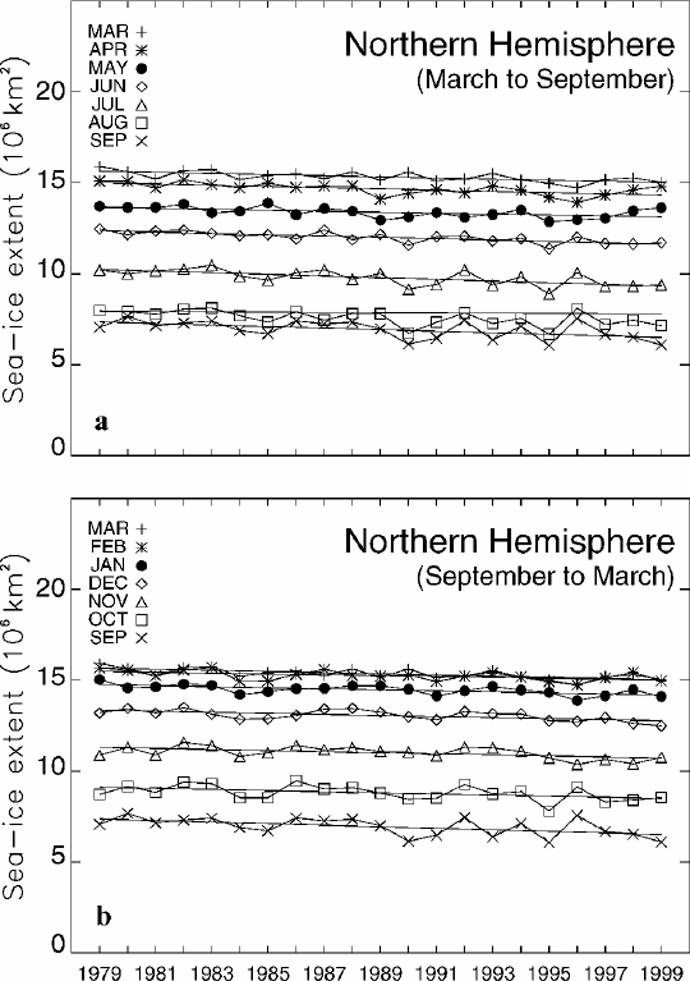
Fig. 2. Time series of monthly sea-ice extents, arranged by month, for the total ice cover of the regions identified in Figure 1. (a) The ice-cover decay, March–September; (b) the ice-cover growth, September–March. Lines of linear least-squares fit are included for each month.

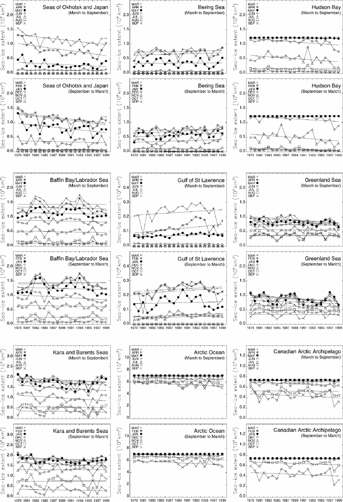
Fig. 3. Time series of monthly sea-ice extents, arranged by month, for each of the nine regions of Figure 1. For each region, the top plot presents the results for March–September, and the bottom plot presents the results for September–March. Lines of linear least-squares fit are included for each month.

The month of minimum ice coverage is consistently September for the Northern Hemisphere as a whole (Fig. 2) and regionally is consistently either August or September except in the cases of the Seas of Okhotsk and Japan and the Gulf of St Lawrence, where the ice cover is reduced to zero for the 3 months July–September, and in the case of Hudson Bay for 1993, when the minimum occurs in October (Fig.3). September is the month of minimum ice coverage in each year for Baffin Bay/Labrador Sea and the Kara and Barents Seas, in each year except 1993 for Hudson Bay, in each year except 1980 and 1997 for the Canadian Arctic Archipelago, in each year except 1980,1987 and 1992 for the Arctic Ocean and in 16 of the 21 years for the Greenland Sea. The one anomalous region is the Bering Sea, in which the month of minimum ice coverage is consistently August rather than September, although with near-zero ice coverage throughout the 4 months July–October (Fig. 3).

The month of maximum ice coverage is considerably more variable than the month of minimum ice coverage. For the Northern Hemisphere as a whole, the month of maximum coverage is March in 17 of the 21 years but February in 1981, 1987, 1989 and 1998 (Fig. 2). Hudson Bay, the Arctic Ocean and the Canadian Arctic Archipelago have their ice extents capping out at the full area of the region for February and March of each year and often for January, December and/or April as well (Fig. 3). In the Seas of Okhotsk and Japan, the month of maximum ice coverage is March for 16 of the years and February for the remaining 5 years; in Baffin Bay/Labrador Sea, it is March for 12 years and February for 9 years; and in the Gulf of St Lawrence, it is February for 16 years and March for 5 years. The variability is greater in the Bering Sea, Greenland Sea and Kara and Barents Seas, in each of which each of the first 4months of the year is the month of maximum for at least one of the years of the 21 year record. In the Greenland Sea, there is even one year (1995) when May is the month of maximum (Fig. 3).

The greater variability observed for the month of maximum ice coverage than for the month of minimum ice coverage results from the presence of ice at lower latitudes during winter. Regions that have open southern boundaries are particularly susceptible to the passage of storms and thus increased variability. For instance, the particularly high variability in the Greenland Sea and the Kara and Barents Seas is almost certainly related to the high frequency and interannual variability in the storm systems in this general area, which tends to experience the strongest and most frequent winter cyclones of the high northern latitudes (e.g. Reference Serreze, Box, Barry and WalshSerreze and others, 1993). Similarly, the Bering Sea is particularly susceptible to variations in the Aleutian Low and associated storm tracks (e.g. Reference Overland and PeaseOverland and Pease, 1982).

Storm systems might also be involved in the prominent increase in variability of summer and early-fall ice extents in the Arctic Ocean region after 1988 (Fig. 3). In fact, Reference Walsh, Chapman and ShyWalsh and others (1996) report marked sea-level pressure reductions over the central Arctic in the period 1987–94 vs the earlier 1979–86 period, and Reference Maslanik, Serreze and BarryMaslanik and others (1996) report an increased frequency of cyclones in the central Arctic starting in 1989. The center of the increase in cyclonic activity was located north of the Laptev Sea, at about 85°N, 120°E (Reference Maslanik, Serreze and BarryMaslanik and others, 1996, fig. 4), in a position to influence directly

summer and fall sea-ice extents in the Arctic Ocean region.

Ice-extent trends

Table 1lists the trends, calculated as the slopes of the lines of linear least-squares fit, in the yearly-averaged ice extents for each of the nine regions of Figure 1, plus the trends in the yearly- and seasonally averaged ice extents for the Northern Hemisphere total. All trends are for the 21 year period 1979–99 and are updated from the 18 year results presented in Reference Parkinson, Cavalieri, Gloersen, Zwally and ComisoParkinson and others (1999). The Northern Hemisphere total continues to show negative trends for each season and for the yearly average, although the overall annual trend has decelerated slightly, by a statistically insignificant 3.2%, from the 18 year value of –34 000±8300 km² a^–1 (–2.8±0.7% per decade) (Reference Parkinson, Cavalieri, Gloersen, Zwally and ComisoParkinson and others (1999)) to –32 900±6100 km² a^–1 (–2.7±0.5% per decade) (Table 1). Summer, defined as in Reference Parkinson, Cavalieri, Gloersen, Zwally and ComisoParkinson and others (1999) as July– September, is the season with the greatest negative trend, both in absolute terms and on a percentage basis, although all four seasons have statistically significant negative trends (Table1).

Regionally, the largest contributor to the negative yearly-average trend is the Arctic Ocean, at –9400±3400km² a^–1, and the next largest contributors are the Kara and Barents Seas (not statistically significant) and the Seas of Okhotsk and Japan (Table 1). When the record had extended only through 1996, the largest contributor to the negative trend was the Kara and Barents Seas, with a trend statistically significant at a 99% confidence level (Reference Parkinson, Cavalieri, Gloersen, Zwally and ComisoParkinson and others (1999)); but relatively high ice extents in the Kara and Barents Seas in 1999 and especially 1998 (Fig.3) weakened the negative slope for that region, while relatively low ice extents in the Arctic Ocean in 1998 and 1999 (Fig. 3) led to a strengthening of its negative trend (Table1 vs Reference Parkinson, Cavalieri, Gloersen, Zwally and ComisoParkinson and others (1999)).

Table 1. Trends (and their standard deviations) in 1979–99 yearly-averaged sea-ice extents for the nine regions of Figure 1 and in 1979–99 yearly- and seasonally averaged sea-ice extents for the Northern Hemisphere total; also, the 21year average extents for each case

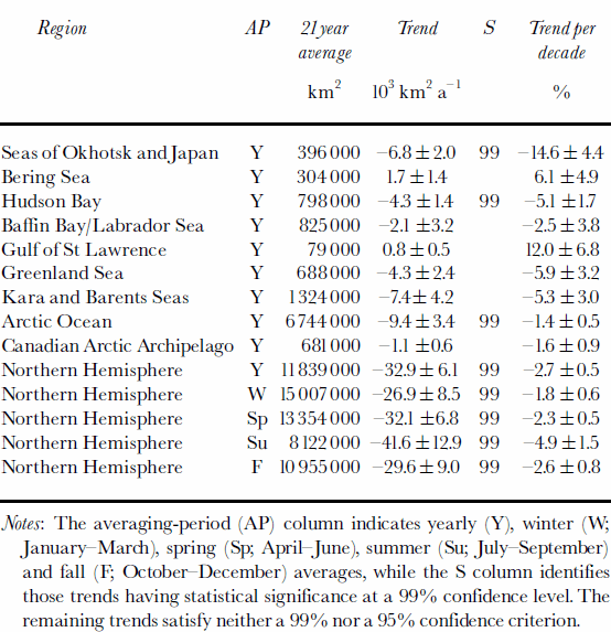
The trend values in each case are the slopes of the lines of linear least-squares fit through the appropriate 21 monthly-average ice extents.

The ice-extent trend values for each month are plotted in Figure 4, for each of the regions and the Northern Hemisphere total. Summer trends are zero in the Seas of Okhotsk and Japan and the Gulf of St Lawrence due to the disappearance of the ice in those regions in each summer; and winter trends are zero in Hudson Bay, the Arctic Ocean and the Canadian Arctic Archipelago due to the complete coverage of each of those regions by ice of at least 15% concentration in the winter months (Fig. 4). In general, with the exception of the zero and near-zero trends, the sign of the trend tends to be the same throughout the year for any individual region; i.e. a region with a negative January trend tends to have negative or zero trends in each month. The two primary exceptions to this are the positive February trend for Baffin Bay/Labrador Sea, a region for which the remaining months have negative or zero trends (Fig. 4d), and the seasonal contrast in the Bering Sea, where the trends are clearly positive in December–April but near zero or negative in May–November (Fig. 4b).

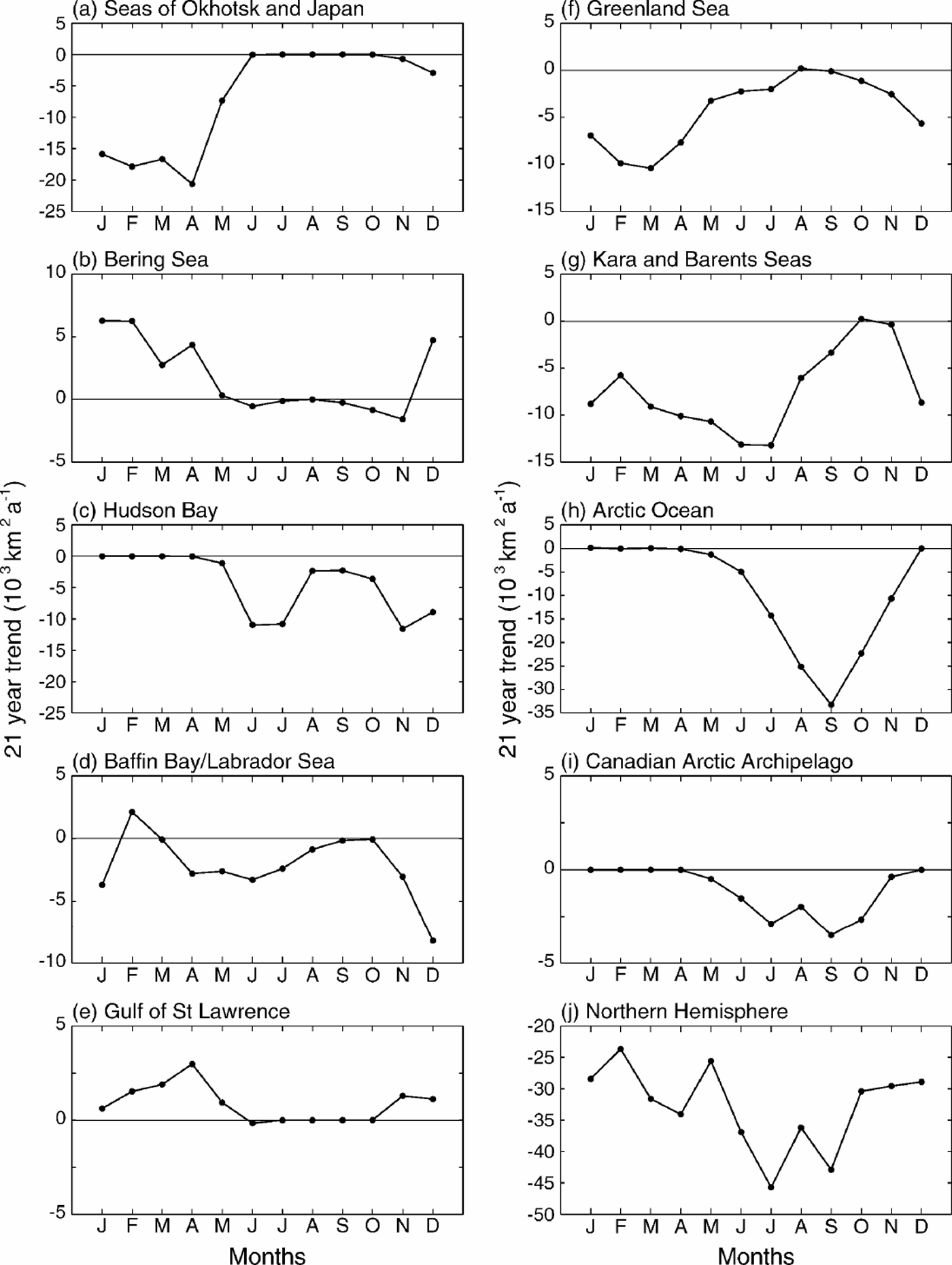
Fig. 4. Trends, by month, in the sea-ice extents of (a–i) the nine regions of Figure 1 and (j) the total, calculated over the 21years1979–99.

The timing of the strongest trends varies from region to region (Fig. 4). For the Arctic Ocean, the ice reductions are strongest in the late summer, with September experiencing reductions, on average, of 33300±13 000 km² a^–1 and the magnitude of the reductions for the rest of the non-winter months being approximately symmetric about the September peak (Fig. 4h). By contrast, reductions in the Kara and Barents Seas peak in June andJuly (Fig. 4g), and those in the Seas of Okhotsk and Japan peak in April (Fig.4a). The varied regional responses combine to a Northern Hemisphere total that has 21 year linear least-squares reductions of at least 23600 km² a^–1 in all 12 months, with the greatest reductions coming in July, at 45700±12200 km² a^–1, and the second greatest in September (Fig. 4j).

From an analysis of Arctic surface air-temperature data for the period 1979–97, Reference Rigor, Colony and MartinRigor and others (2000) report seasonal and spatial trends in their data that are generally consistent with the sea-ice extent trends shown in this study. For December–February they report a warming trend over the Eurasian land mass and over the Laptev and East Siberian Seas to the north of Russia, whereas for eastern Siberia and north of the Canadian Arctic Archipelago they report cooling trends. During September–November, the regions showing cooling trends are Alaska and the Beaufort Sea. March–May show warming trends over the entire Arctic region. During June–August, however, there are no significant trends in the temperature data (Reference Rigor, Colony and MartinRigor and others, 2000), which is interesting because June–September are the months for which we find the strongest negative trends for the ice cover as a whole (Fig. 4j).

Discussion

Satellite technology provides a powerful resource for monitoring the Arctic sea-ice cover’s distribution and extent, and we have taken advantage of this by using this technology to quantify changes in the Arctic ice cover since the late 1970s, with results presented in Table 1 and Figures 2–4 for the 21 year period 1979–99. Most notably, the ice cover as a whole has negative trends for every month, with a trend in the annual averages of –32 900±6100 km² a^–1.

Because of the sharp contrast between the microwave emissivities of liquid water and ice, the satellite passive-microwave data are particularly good at revealing the distribution of the sea-ice cover, which in turn allows calculation of the ice extent and determination of changes in ice extent. These satellite data are not as appropriate for determining changes in ice thickness, but analyses of submarine data have revealed a thinning of the ice cover (e.g.Reference Rothrock, Yu and MaykutRothrock and others, 1999) that is even more dramatic, percentage-wise, than the ice-extent reductions reported here. (However, Reference WinsorWinsor (2001) reports that the thinning did not continue in the 1990s, at least over a limited region from north of Alaska to the North Pole.)

Of course neither the satellite data nor the submarine data can explain the causes of the sea-ice changes or predict future changes. If the decreasing ice coverage is tied most closely to an ongoing Arctic warming (Reference Martin, Munoz and DruckerMartin and others, 1997; Reference SerrezeSerreze and others, 2000) that continues, then the ice cover is likely to continue to decrease as well; but if the sea-ice changes are tied more closely to oscillatory behaviors in the climate system, such as the North Atlantic Oscillation and the Arctic Oscillation (as suggested by, e.g., Reference Deser, Walsh and TimlinDeser and others, 2000; Reference Morison, Aagaard and SteeleMorison and others, 2000; Reference ParkinsonParkinson, 2000), then it is likely that there will also be fluctuations between periods of sea-ice decrease and periods of sea-ice increase.