


Introduction
Forests affect the climate through several mechanisms, such as water cycles, greenhouse gas fluxes, aerosols, and surface albedoFootnote 1 (Myhre et al. Reference Myhre, Shindell, Bréon, Collins, Fuglestvedt, Huang, Koch, Lamarque, Lee, Mendoza, Nakajima, Robock, Stephens, Takemura, Zhang, Stocker, Qin, Plattner, Tignor, Allen, Boschung, Nauels, Xia, Bex and Midgley2013; Smith et al. Reference Smith, Bustamante, Ahammad, Clark, Dong, Elsiddig, Haberl, Harper, House, Jafari, Masera, Mbow, Ravindranath, Rice, Robledo Abad, Romanovskaya, Sperling, Tubiello, Edenhofer, Pichs-Madruga, Sokona, Farahani, Kadner, Seyboth, Adler, Baum, Brunner, Eickemeier, Kriemann, Savolainen, Schlömer, von Stechow, Zwickel and Minx2014). Here, we focus on two mechanisms that force the climate in opposite directions: carbon storage and surface albedo. Removing carbon from the atmosphere cools the climate. Increasing carbon storage in biomass, products, and soils has been therefore proposed as a way to mitigate climate change. Nevertheless, increasing carbon storage means expanding forest area or density, both of which reduce Earth's albedo (i.e., make Earth's surface darker). Dark surfaces absorb more solar radiation than light surfaces. Thus, making Earth's surface darker warms the climate. There is a tradeoff between the cooling impact of increased carbon storage and the warming impact of decreased albedo, especially in the boreal regionFootnote 2 (Betts Reference Betts2000). In economics, these climatic impacts are considered an externality of forestry. Carbon storage and albedo can be optimally regulated by pricing them according to their social value (Pigou Reference Pigou1920, Thompson, Adams, and Sessions Reference Thompson, Adams and Sessions2009). In this way, their social value becomes internalized in private landowners’ management decisions. Here, we consider the market-level implications of the joint regulation of carbon and albedo on land allocation, carbon storage, and timber harvests and prices.
Stand-level forest management for timber, carbon, and albedo has been previously studied by Thompson, Adams, and Sessions (Reference Thompson, Adams and Sessions2009), Lutz and Howarth (Reference Lutz and Howarth2014), Lutz and Howarth (Reference Lutz and Howarth2015), Lutz et al. (Reference Lutz2016), and Matthies and Valsta (Reference Matthies and Valsta2016). However, the stand-level approach has two important limitations. First, the timber price is treated as a fixed exogenous parameterFootnote 3, although in reality, prices react to policies (such as carbon and albedo pricing) that affect the timber supply. A market-level model is needed to capture these price effects that also influence stand-level forest management. Second, stand-level models depict the management of a single land parcel in a fixed use and therefore cannot be used to examine land use change. However, because pricing carbon and albedo alters the value of land in forestry and agriculture, it is likely to encourage land use change. A market-level model is needed to understand these land-use effects that contribute to the climatic impacts of joint regulation.
To our knowledge, only one study so far has addressed the market-level implications of joint regulation. Sjølie, Latta, and Solberg (Reference Sjølie, Latta and Solberg2013a) consider the issue in the context of the Norwegian forest sector. Our approach differs from theirs in two ways. First, Sjølie, Latta, and Solberg (Reference Sjølie, Latta and Solberg2013a) do not consider land use change; their model only includes forest land. Our model includes a competing land use (agriculture). This allows us to study the policy's land-use implications. Second, while Sjølie, Latta, and Solberg (Reference Sjølie, Latta and Solberg2013a) consider the impacts of the regulation in a specific, highly detailed geographical context, we look at the question in a more abstract setting. This allows us to freely explore how the policy's impacts depend on our modelling assumptions.
We conduct our analysis using a partial equilibrium market-level model with two land uses (forestry and agriculture) and markets for two goods (timber and crops). Forests are age structured. Carbon fluxes and surface albedo are priced according to their social value (Lutz and Howarth Reference Lutz and Howarth2014). The general structure of our model is based on a market-level model by Salo and Tahvonen (Reference Salo and Tahvonen2004) that includes two land uses but no externalities. The model has been extended to include carbon by Cunha-e-Sá, Rosa, and Costa-Duarte (Reference Cunha-e-Sá, Rosa and Costa-Duarte2013), Lintunen and Uusivuori (Reference Lintunen and Uusivuori2016), Rautiainen, Lintunen, and Uusivuori (Reference Rautiainen, Lintunen and Uusivuori2017), and Tahvonen and Rautiainen (Reference Tahvonen and Rautiainen2017).Footnote 4 Here, we extend it to include both carbon and albedo. In line with projections made using global integrated assessment models (e.g., Nordhaus Reference Nordhaus2014), we allow carbon and albedo pricesFootnote 5 to change over time.
The rest of the article is organized as follows. First, we outline our market-level model and derive rules that characterize optimal land allocation and harvests and, thus, define how land use and forest age structure change over time. Then, we analyze an artificial market-level steady-state solution, applying the same standard assumptions that have been previously applied in stand-level analyses. In other words, we assume (1) time-invariant prices, (2) a fixed land allocation, and (3) the existence of a unique optimal rotation. The results from stand-level models formulated in this context (e.g., Thompson, Adams, and Sessions Reference Thompson, Adams and Sessions2009) suggest that it is optimal to manage forests according to a Hartman rotation (Hartman Reference Hartman1976) that takes into account both externalities. We show that the same result can be obtained from our market-level model, if the same (restrictive) static-world assumptions are applied. This highlights the theoretical connection of our market-level results and previous stand-level studies.
We then relax the steady-state assumptions and solve the model in a (more realistic) dynamic setting, in which prices, land use, and forest age structure are allowed to change over time. In this setting, it is no longer meaningful to assume the existence of a single optimal rotation. Rather, it may be optimal to harvest wood from various age classes at the same time. We numerically simulate the temporal development of the land-use system with alternative climate policies and discounting schemes. We focus on four factors: land allocation, climatic impacts, timber harvests, and timber prices. We compare the impacts of imperfect (carbon-only or albedo-only) regulation with comprehensive (carbon and albedo) regulation, and the status quo in which forests’ climatic impacts are not regulated. We show that carbon pricing leads to an overprovision of climate benefits at the expense of food and timber production. Complementing the policy with albedo pricing reduces these welfare losses, as it limits the afforestation of agricultural land and maintains harvests at a higher level. Furthermore, we show that the outcome of the optimal regulation is sensitive to the strength of the albedo effect (i.e., how much the warming power of a hectare of mature forest differs from that of treeless land), the productivity of the forest land and the stringency of the applied climate policy. We discuss the policy implications of our results and the limitations of this study.
Model
Model Overview, Underlying Assumptions, and Solution Concept
We develop a partial equilibrium model of a small economy. The model consists of a description of the markets for two goods (crops and timber) and the land use system that produces them. The demand for the goods is depicted by two separate exogenous inverse demand functionsFootnote 6. The supply of the goods is determined endogenously as a result of land use decisions. Crop supply in each time period depends on the extent of the land area allocated to agriculture. Timber supply is determined by age-class-specific clear-cutting decisions.
The climatic impacts of land use are regulated. Albedo is priced based on the social cost of forcing (SCF) and the warming power of the land coverFootnote 7, as in Lutz and Howarth (Reference Lutz and Howarth2014). The SCF is the global monetary value of the social damage caused by marginal radiative forcing at a given instant (Wm−2). Rautiainen and Lintunen (Reference Rautiainen and Lintunen2017) outline how the social cost of any forcing agent whose temporal decay profile and radiative efficiency are known can be calculated based on the SCF. Carbon fluxes are priced according to a the Social Cost of Carbon (SCC), which is the monetary value of the global social damage caused by a marginal ton of CO2 emitted into the atmosphere at a given date. The carbon and albedo prices in the analytical model are generic. The specific SCC and the SCF values used in the numerical examples (later on) are both from Rautiainen and Lintunen (Reference Rautiainen and Lintunen2017), where the SCC trajectory is calculated based on the SCF trajectory. This guarantees that the prices of carbon and albedo are mutually consistent. That is, the same social cost is associated with a warming impact of a similar magnitude, occurring at the same point in time, regardless of whether it is caused by carbon or albedo.
The SCC and SCF are measures of global marginal damageFootnote 8. These marginal damages are determined by the total amount of anthropogenic radiative forcing. Because the economy depicted by our model is small compared to the global economy, it contributes only marginally to total anthropogenic radiative forcing. Its ability to influence global SCC and SCF values is therefore negligible, and these prices can be safely depicted by exogenous trajectoriesFootnote 9.
The market equilibrium is solved as a social welfare maximization problem. In this study, social welfare is defined as economic surplus (i.e., the sum of consumer and producer surpluses) plus the social value of the climate externality.Footnote 10 From basic microeconomic theory we know that (in the absence of market failures) welfare is maximized at the market equilibrium. Thus,—thinking conversely—the market equilibrium can be found by maximizing surplus. The aggregate market-level behavior described by the applied model type is the same as the behavior that emerges when the land use and consumption decisions are made by separate price-taking agents (Lintunen and Uusivuori Reference Lintunen, Laturi and Uusivuori2016). Market-level phenomena can therefore be analyzed without explicitly modelling landowner and consumer behavior. We make use of this property. We present and solve the model as a social planner's welfare maximization problem (which is simpler than separately modelling producers and consumers) but interpret the outcome as a market equilibrium. Moreover, as we do not model the behavior of individual agents, we do not explicitly need to define how the incentives to regulate carbon and albedo are decentralized to private landownersFootnote 11. It suffices that all climatic impacts are priced consistently and comprehensively in the social welfare maximization problem.
The model is intended to be parsimonious: we have restricted its features to the bare essentials required for understanding the market-level impacts of joint regulation. Some examples of the simplifying assumptions applied in the model are: the inclusion of only two land uses, the omission of land use conversion costs, a simplified representation of the soil carbon stocks and the exclusion of the possibility to use logging residues for bioenergy. All of these features can be modelled in more detail (see, e.g., Rautiainen, Lintunen, and Uusivuori (Reference Rautiainen, Lintunen and Uusivuori2017)). However, as they are not essential to developing an understanding of the general principles of the optimal regulation, they are omitted for clarity.
Model set-up
Land Allocation and Harvests
The extent of total land area is normalized to one unit. There are two land uses: agriculture and forestry. Agriculture produces agricultural crops and forests provide timber. Agricultural area in period t ∈ {1, 2, …} is denoted by y t ≥ 0. Forests are divided into age classes, a ∈ {1, 2, …}; the area of each age class is denoted by x at. All timber harvests are clear cuts. The area z at is harvested from class a ≥ 1. Harvests take place at the beginning of each period, and the cleared forest land may be allocated to either land use. Total bare land available after timber harvest is  $y_{t - 1} + \sum\nolimits_{a = 1}^\infty \; {z_{at}} $, and it can be allocated to agricultural use for that period, y t, or planted to grow forest. An auxiliary age-class $x_t^0 $ denotes the area of new stands established in a given period. The land use dynamics are summarized by Equations (1)–(3).
 $$ x_t^0 + y_t = \; y_{t - 1} + \; \mathop \sum \limits_{a = 1}^\infty z_{at}\; \forall \; t$$
 $$x_{a + 1,t + 1} = x_{at} - z_{at\; \;} \forall a \ge 1,\; \; \; {\rm and}\; \; \; x_{1,t + 1} = x_t^0 $$
 $$y_t \ge 0\comma \; \; x_t^0 \ge 0, \;\;{\rm and} \; \; \; x_{at} \ge z_{at} \ge 0\; \; \forall \; t$$
 The crop yield per unit area, b, is constant. Thus, crop harvest  $\tilde{h}_t$ is
 $$\tilde{h}_t = \; by_t.$$
 The per-hectare timber volume (m3), v a, increases with stand age (i.e.,  $ v_{a + 1} \gt v_a\forall a$). The total harvested timber volume (m3), h t, is
 $$h_t = \mathop \sum \limits_{a = 1}^\infty v_az_{at}.$$
However, timber from different age classes is valued differently in the markets: young stands produce less valuable timber grades than old stands. Hence, we specify quality weighted harvests
 $$q_t = \mathop \sum \limits_{a = 1}^\infty {\rm \sigma} _av_az_{at}\comma \; $$
where the parameters σa ∈ (0, 1) are quality weights. We assume that quality improves as the stand ages, i.e., σa+1 >σa.
Climatic Impacts of Land Use
Land use affects the climate through surface albedo and carbon storage. Surface albedo depends on the current land cover. Its climatic impact can be expressed as mean annual warming power (hereafter, simply warming power), measured in MWha−1. Bright, Strømman, and Peters (Reference Bright, Strømman and Peters2011) describe how warming power can be calculated based on the top-of-the-atmosphere net shortwave (SW) fluxFootnote 12.
We assume that the warming power of forest, w a, depends on stand age. The warming power of a recently established forest stand, w 0, is equal to that of open shrub. Lukeš, Stenberg, and Rautiainen (Reference Lukeš, Stenberg and Rautiainen2013) identify a negative relationship between stand albedo and biomass for boreal coniferous forests. In our model, biomass increases—and, thus, albedo decreases– with stand age. We therefore assume that warming power increases with stand age, i.e.,  $w_a \lt w_{a + 1}\; \forall \; a$. In line with Lukeš, Stenberg, and Rautiainen (Reference Lukeš, Stenberg and Rautiainen2013), the increases in warming power between age classes diminish as the canopy closes, i.e., w a+2 − w a+1 < w a+1 − w a. We assume that the warming power of agricultural land, w y, is constant and equal to the warming power of open shrub (w y = w 0). The total warming power of the land surface in period, W t, is
 $$W_t = w_0\lpar{x_t^0 + y_t} \rpar+ \mathop \sum \limits_{a = 1}^\infty w_a\lpar x_{at} - z_{at}\rpar .$$
 The net change in the terrestrial carbon stock,  ${\rm \Delta} _t^C $, indicates the net flux between ecosystems and the atmosphere (i.e., ${\rm \Delta} _t^C \; \gt 0 $ means net removals, ${\rm \Delta} _t^C \; \lt 0 $ means net emissions). ${\rm \Delta} _t^C $ includes changes in carbon stored in biomass, $\Delta _t^B $, soils, $\Delta _t^S $, and wood products, $\Delta _t^P $, i.e.,
 $$\Delta _t^C = \Delta _t^B + \Delta _t^S + \Delta _t^P. $$
Formally, the biomass carbon stock changeFootnote 13 is
 $$\Delta _t^B = \lpar \gamma _v + \gamma _b\rpar \left[ {\mathop \sum \limits_{a = 1}^\infty \lpar v_{a + 1} - v_a\rpar x_{at} + v_1x_t^0 - \mathop \sum \limits_{a = 1}^\infty v_{a + 1}z_{at}} \right] , $$
where γ v ∈ ℝ+ is the carbon density of timber, and γ b ∈ ℝ+ is the carbon content of other woody biomass proportional to the timber volume.
When a stand is cut, the carbon contained in biomass is transferred into products (as timber) and soils (as residues). Wood products (e.g., paper wrappers and furniture) have different lifespans. The share of carbon contained in goods produced in period t and released in period t + j is denoted by  ${\rm \delta} _j^P \; \ge 0$ (where j ∈ {0, 1, …} and $\sum\nolimits_{j = 0}^\infty \; {{\rm \delta} _j^P \; = 1} $). Logging residues (that are left on site) decompose and release carbon over time. The share of the carbon in residues generated in period t released in period t + j is denoted by ${\rm \delta} _j^S \; \ge 0$, (where j ∈ {0, 1, …} and $\sum\nolimits_{j = 0}^\infty \; {{\rm \delta} _j^S \; = 1} $). We obtain,
 $$\Delta _t^P + \Delta _t^S = \gamma _v\bigg({h_t - \mathop \sum \limits_{\,j = 0}^\infty {\rm \delta} _j^P h_{t - j}} \bigg)+ \gamma _b\bigg({h_t - \mathop \sum \limits_{\,j = 0}^\infty {\rm \delta} _j^S h_{t - j}} \bigg).$$
Economic Optimization
Timber and crops are consumed in the same period in which they are harvested. Thus, consumption equals harvests. The (separable) inverse demand functions for timber and crops are p(q t) and  $\tilde{p}\lpar \tilde{h}_t\rpar $. We assume $p \gt 0\comma \; p^{\rm {\prime}} \lt 0\comma \; p^{\rm \prime \prime} \le 0\, \forall q_t \ge 0$ and $\tilde{p} \gt 0\comma \; \tilde{p}^{\rm {\prime}} \lt 0\comma \; \tilde{p}^{\rm \prime \prime} \le 0\, \forall \; \tilde{h}_t \ge 0$. The gross social welfareFootnote 14 from consuming timber, U t, is obtained by integrating p, i.e, $U_t = U\lpar q_t\rpar := \,\,\int_0^{q_t} {p\lpar h\rpar dh} $. Likewise, the gross social welfare from consuming crops is $ \tilde{U}_t = \tilde{U}\lpar \tilde{h}_t\rpar := \,\,\int_0^{{\tilde{h}}_t} {\tilde{p} \lpar h \rpar dh} $. We observe that $U^{\rm {\prime}} = p \gt 0\comma \; U^{\prime\prime} = p^{\rm {\prime}} \lt 0\comma \; \; \tilde{U^{\rm {\prime}}} = \tilde{p}\gt 0$ and $\hskip-3pt \tilde{\hskip--3pt U^{\rm \prime \prime}} = \tilde{p^{\rm {\prime}}} \lt 0$.
The timber and crop prices are determined endogenouslyFootnote 15. The carbon price,  $p_t^c $, and the price of albedo warming power, $p_t^w $, are exogenousFootnote 16. The harvesting costs for timber and crops (per unit harvested) are c h and $\tilde{c}_h$, respectively. Forest regeneration costs (per area) are c r. The crop production costs per hectare are c f. The total costs accrued in each period, C t, are
 $$C_t = c_hh_t + \tilde{c}_h\tilde{h}_t + c_rx_{t}^{0} + c_fy_t.$$
The social planner aims to maximize social welfare, i.e., the economic surplus from crop and timber consumption plus the social value of climatic impacts of land use. Welfare from future periods is discounted by the discount factor β ∈ (0, 1). The initial land allocation, x a0, …, x n0, y 0 is exogenous, but in later periods it is determined by the planner's choices. In each period the planner decides how much land to allocate to each land use and how much forest to cut from each age class. The planner's objective function is
 $$\mathop {{\rm max\; }} \limits_{D} J(D) = \mathop \sum \limits_{t = 0}^\infty B_{0t} \left[ {U\lpar q_t\rpar + \tilde{U}\lpar {\tilde{h}}_t\rpar + p_t^c \Delta _t^C - p_t^w W_t - C_t} \right], $$
where  $ D = \{D_t \;\vert \; \forall t \} \; {\rm and}\; D_t = \left\{{x_t^0\comma \; x_{a\comma t + 1}\comma \; y_t\comma \; z_{at}\; \forall \; a} \right\}\!, s.t. (1)\!\!-\!\!(11) $. We include a time-variant discount factor $B_{st}:= \prod\nolimits_{u = s}^{t - 1} {{\rm \beta} _u} $, where βu is the discount factor in period u, and B tt = 1, for all t. The Lagrangian function of the problem is
 $$\eqalign{L\lpar D\comma \; {\rm \lambda}^b\comma \; {\rm \lambda}^f\comma \; {\rm \mu}^{\bar z}\rpar = &\,J(D) + \mathop \sum \limits_{t = 0}^\infty B_{0t}{\rm \lambda} _t^b \bigg({y_{t - 1} + \; \mathop \sum \limits_{a = 1}^\infty z_{at} - y_t - x_t^0} \bigg)\cr & + \mathop \sum \limits_{t = 0}^\infty B_{0\comma t + 1}{\rm \lambda} _{1\comma t + 1}^f \bigg({x_t^0 - x_{1\comma t + 1}} \bigg) \cr & + \mathop \sum \limits_{t = 0}^\infty \mathop \sum \limits_{a = 1}^\infty B_{0\comma t + 1}{\rm \lambda} _{a + 1\comma t + 1}^f \bigg( x_{at} - \; z_{at} - x_{a + 1\comma t + 1}\bigg) \cr & + \mathop \sum \limits_{t = 0}^\infty \mathop \sum \limits_{a = 1}^\infty B_{0t}{\rm \mu} _{at}^{\bar z} \bigg( x_{at} - \; z_{at}\bigg) \comma \; } $$
where we have omitted the non-negativity constraints. The Lagrangian function of the welfare maximization problem (in a less concise form) and the necessary first order conditions for optimum are given in Appendix 1 [(A1)–(A8)].
Characterization
Optimal Land Allocation and Harvests
The Lagrangian multiplier  $\lambda _t^b $ is the value of bare land. Bare land may be allocated to either use. If land is allocated to both forestry and agriculture in the same period, the marginal unit of bare land has the same value in either use. The optimality conditionFootnote 17 for allocating bare land to agriculture, y t, is
 $$\lpar \tilde{U}^{\prime}\lpar \tilde{h}_t\rpar - \tilde{c}_h\rpar b - p_t^w w_y + {\rm \beta} _t\lambda _{t + 1}^b \le \lambda _t^b. $$
 The left hand side (LHS) of (14) is the value of agricultural land, which consists of the harvesting profits,  $\lpar \tilde{U}^{\prime}\lpar \tilde{h}_t\rpar - \tilde{c}_h\rpar b$, the social cost of the warming impact of surface albedo, $p_t^w w_y$, and the discounted value of bare land in the next period (i.e., when the land is reallocated to a new use after one crop rotation), ${\rm \beta} _t{\rm \lambda} _{t + 1}^b $. If this value is less than the current bare land value, ${\rm \lambda} _t^b $, no land is allocated to agriculture and the bare land value is determined by the other use (forestry). If a positive amount of land is allocated to agriculture, equation (14) holds as an equality.
The multiplier  ${\rm \lambda} _{at}^f $ is the social value of forest in age class a, i.e., the discounted value of the net benefit stream from the stand. The optimality condition for allocating bare land to forestry, x 0t, is
 $$ - c_r + \beta _t\lambda _{1\comma t + 1}^f + p_t^c \lpar{\gamma _v + \gamma _b} \rpar v_1 - p_t^w w_0 \le \lambda _t^b.$$
 The LHS of (15) is the value of a newly established forest stand. It consists of the discounted future timber income stream net of regeneration costs,  $ - c_r + {\rm \beta} _t{\rm \lambda} _{1\comma t + 1}^f $, and the social value of the climatic impacts of carbon sequestration and albedo in period $t\comma \; p_t^c \lpar {\rm \gamma} _v + {\rm \gamma} _b\rpar v_1 - p_t^w w_0$. If the value of forested land is less than the current bare land value, ${\rm \lambda} _t^b $, no bare land is allocated to forestry. However, if a positive amount of bare land is allocated to forestry, then equation (15) holds as an equality.
The value of forested land,  ${\rm \lambda} _{at}^f $, is based on the future income streams that the stand provides when it is used for forestry. The value of a stand is recursively given by equation
 $${\rm \lambda} _{at}^f \ge p_t^c \lpar {\rm \gamma} _v + {\rm \gamma} _b\rpar \lpar v_{a + 1} - v_a\rpar - p_t^w w_a + {\rm \beta} _t{\rm \lambda} _{a + 1\comma t + 1}^f + {\rm \mu} _{at}^{\bar z}\comma \; $$
which holds as an equality if the area of the age-class, x at, is positive. The stand-value (RHS) consist of current net climate benefits,  $p_t^c \lpar {\rm \gamma} _v + {\rm \gamma} _b\rpar \lpar v_{a + 1} - v_a\rpar - p_t^w w_a$, and the future value of the stand if it is left to grow, ${\rm \beta} _t{\rm \lambda} _{a + 1\comma t + 1}^f $, or harvest value, if it is harvested ${\rm \beta} _t{\rm \lambda} _{a + 1\comma t + 1}^f \; + {\rm \mu} _{at}^{\bar z}. $ The description of the value dynamics of forest land is not complete without the optimality condition for the harvest decision. The optimal harvesting condition is
 $$\lpar U^{\rm {\prime}}\lpar h_t\rpar - c_h\rpar v_a - {\rm K}_{at} + {\rm \lambda} _t^b - {\rm \beta} _t{\rm \lambda} _{a + 1\comma t + 1}^f - {\rm \mu} _{at}^{\bar z} \le 0\comma \; $$
where (U ′(h t) − c h)v a gives the marginal profit from the harvest and
 $${\rm K}_{at}:= p_t^c \lpar v_{a + 1} - v_a\rpar \lpar {\rm \gamma} _v + {\rm \gamma} _b\rpar + v_a\mathop \sum \limits_{\,j = 0}^\infty B_{t\comma t + j}p_{t + j}^c \lpar{{\rm \gamma} _v{\rm \delta} _j^P + {\rm \gamma} _b{\rm \delta} _j^S} \rpar- p_t^w w_a$$
denotes the climate costs of harvesting. The first term on the RHS in (18) denotes forgone carbon sequestration (due to not leaving the stand to grow for one more period). The second term denotes the current and future emissions from wood use and the eventual oxidation of wood product and soil carbon pools. The third term is the avoided albedo warming.
The interpretation of the optimal harvesting condition (17) is as follows. In addition to harvest profits and climate costs, harvesting clears land for reallocation: the value of bare land is  ${\rm \lambda} _t^b $. If the sum of these three values is equal to or higher than the present value of the stand when it is allowed to grow for one more period, ${\rm \beta} _t{\rm \lambda} _{a + 1\comma t + 1}^f $, then at least some of the age class is harvested. If it is optimal to harvest the whole age-class, the Lagrange multiplier ${\rm \mu} _{at}^{\bar z} $ kicks in and enforces the non-positivity of the equation. Otherwise, ${\rm \mu} _{at}^{\bar z} \; = 0$. In an optimal interior solution (where z at<x at), the landowner is indifferent between cutting the marginal unit of forest [the value of this option is captured by the first three terms on the RHS in (17)] and keeping it forested (this opportunity cost is captured by the fourth term on the RHS, i.e., $\beta _t\lambda _{a + 1\comma t + 1}^f $).
The value of land in both uses is decreased by the warming impact of albedo [(14) and (16)]. Carbon sequestration acts as an opposite force (16). These two forces also contribute to the optimal timber harvest decision (17): the clear-cutting stops the carbon sequestration and releases the sequestered carbon with a given time profile, but prevents albedo warming caused by a dense forest stand. The relative effect of these forces is determined by the natural properties of the stand (stand growth, carbon release from carbon pools and the strength of albedo's warming power), and the prices assigned to carbon and albedo. The interplay of the natural processes and the prices of the externalities determines the optimal harvesting behavior and land use.
Steady-State Properties of the Model
Previous studies on forest management for timber, carbon and albedo have predominantly focused on stand-level even-aged forestry, usually assuming constant prices and a fixed land allocation. The optimal solution in this context is a Hartman rotation (Hartman Reference Hartman1976) that takes the carbon and albedo externalities into account (Thompson, Adams, and Sessions. Reference Thompson, Adams and Sessions2009). As the surrounding world is (assumed to be) static, the optimal rotation is time-invariant. Here, we show that the same result can be obtained from our market-level model, if similar assumptions are applied.
In the following, we consider an (artificial) steady-state in which (1) land is allocated to both agriculture and forestry, and (2) a unique optimal rotation, a*, exists. We assume that land use change does not occur (all cleared forest and farmland is allocated back to the same use). As the steady-state values of all variables are constant, we drop the time index t from our notation. The steady-state bare land value (BLV) of forest (derived in Appendix 2) is
 $$\eqalign{{\rm \lambda} ^b = & \displaystyle{{ - c_r + \; {\rm \beta} ^{a^{\ast}}v_{a^{\ast}} \left[ {U^{\rm {\prime}}\lpar h\rpar {\rm \sigma} _{a^{\ast}} - c_h} \right] } \over {1 - {\rm \beta} ^{a^{^\ast}}}} - \displaystyle{{\,p^w\mathop \sum \nolimits_{a = 0}^{a^{\ast} - 1} {\rm \beta} ^aw_a} \over {1 - {\rm \beta} ^{a^{\ast}}}} \cr & + \displaystyle{{\,p^c\mathop \sum \nolimits_{a = 0}^{a^{\ast} - 1} {\rm \beta} ^a\lpar {\rm \gamma} _v + {\rm \gamma} _b\rpar \lpar v_{a + 1} - v_a\rpar } \over {1 - {\rm \beta} ^{a^{\ast}}}} - \displaystyle{{{\rm \beta} ^{a^{\ast}}v_{a^{\ast}}p^c\mathop \sum \nolimits_{\,j = 0}^\infty {\rm \beta} ^j\lpar{\gamma _v{\rm \delta} _j^P + {\rm \gamma} _b{\rm \delta} _j^S} \rpar} \over {1 - {\rm \beta} ^{a^{\ast}}}}.} $$
The first term on the RHS of (19) is the Faustmann formula (Faustmann Reference Faustmann1849, Samuelson Reference Samuelson1976). The second term captures the impact of forest albedo on land value. The two last terms indicate the value of carbon storage. The first one accounts for carbon removals by growing biomass (before harvest). The second accounts for the emissions from soils and products (after harvest). Together the four terms constitute a variant of the Hartman formula (Hartman Reference Hartman1976) with two externalities (carbon and albedo), much like in Thompson, Adams, and Sessions (Reference Thompson, Adams and Sessions2009).
The steady-state value of (bare) agricultural land, obtainedFootnote 18 from (13), is
 $${\rm \lambda}^b = \displaystyle{{\lpar \tilde{U}^{\prime}\lpar \tilde{h}\rpar - {\tilde{c}}_h\rpar b - c_f - p^ww_0} \over {1 - {\rm \beta}}}. $$
The first term on the RHS is the discounted stream of profits from crop production over an infinite time horizon. The second term on the RHS is the social cost of the warming impact of the albedo of agricultural land. In an equilibrium in which it is optimal to allocate land to both uses, the value of agricultural land (19) is equated with forest BLV (18).
Quantitative Assessment
Set-up
In reality, the world is not at a steady state. If carbon and albedo pricing are introduced, the land use system will dynamically adjust over time. In this section, we analyze this adjustment. Alternative policies’ land use sector impacts depend on economic parameters (e.g., discount rates, carbon and albedo prices) and physical parameters (e.g., albedo strength and site productivity). We numerically illustrate these dependencies.
For this purpose, the model presented in the previous section was written in GAMS and solved using the CONOPT3 solver by directly maximizing the intertemporal objective function (12) subject to the model's constraints. As solving the model over an infinite time horizon is not technically feasible, the model was solved over a 500-year timespan (i.e., 100 5-year periods). Usually, a steady state is reached by the midpoint of the simulation, if the interest rate, and carbon and albedo prices are held constant. We present the results for only the first 300 years of the simulation (as these results are not yet affected by the nearing end of the simulation time horizon).
The growing conditions in the numerical examples resemble a relatively productive site in Central Finland. (A sensitivity analysis is conducted with a growth description that depicts weaker growing conditions in Northern Finland). Land area in the model is normalized to 1 hectare.Footnote 19 The model is calibrated so that in the no-climate-policy steady state (which is also the initial state of the model), half of the land is allocated to agriculture,Footnote 20 while the other half is forest. Initially, forests have a uniform age distribution, which is characterized by an optimal rotation of 50 years (supported by the equilibrium timber price is 55 €m−3 and a 5 percent interest rate).Footnote 21 The specific technical assumptions regarding stand growth, carbon storage, albedo and the economic parameters are discussed in the Supplementary material.
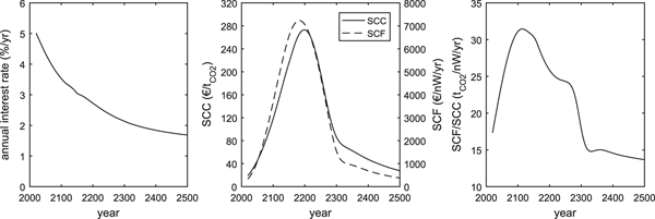
Carbon fluxes are priced based on the SCC. Albedo is priced based on the SCF (Rautiainen and Lintunen Reference Rautiainen and Lintunen2017) and the warming power of the land cover, as in Lutz and Howarth (Reference Lutz and Howarth2014).Footnote 22 In our examples, we consider two distinct discounting and externality pricing schemes. In the first scheme (hereafter “changing prices”), we assume a declining interest rateFootnote 23 and changing SCC and SCF values. The trajectories, obtained from Rautiainen and Lintunen (Reference Rautiainen and Lintunen2017), are shown in Fig. 1. The trajectories have been derived using the DICE 2013R modelFootnote 24 (Nordhaus and Sztorc Reference Nordhaus and Sztorc2013). In the second externality pricing scheme (here after, constant prices) we assume a constant interest rate (5 percent) and constant SCC and SCF values (18.96 €/tCO2 and 328.41 €/nW, respectively) that correspond to the values given for the year 2015 in the changing prices scheme.

Figure 1. The changing interest rate, the SCC and SCF values applied in the calculations and the changing ratio SCF/SCC over time.
The two alternative pricing schemes make our results easier to compare with those of previous studies. Results from Integrated Assessment Models (IAMs) suggest that it is optimal to tighten climate policy over time, as in the “changing prices” scenario (United States Government 2015). This pricing convention is followed by Lutz and Howarth (Reference Lutz and Howarth2014, Reference Lutz and Howarth2015) and Lutz et al. (Reference Lutz2016). However, other previous stand-level studies regarding forest management for timber, carbon and albedo (Thompson, Adams, and Sessions Reference Thompson, Adams and Sessions2009, Matthies and Valsta Reference Matthies and Valsta2016) and market-level studies focusing on carbon pricing (Cunha-e-Sá, Rosa, and Costa-Duarte Reference Cunha-e-Sá, Rosa and Costa-Duarte2013, Sjølie, Latta, and Solberg Reference Sjølie, Latta and Solberg2013b, Lintunen and Uusivuori Reference Lintunen and Uusivuori2016, Tahvonen and Rautiainen Reference Tahvonen and Rautiainen2017) and carbon and albedo pricing (Sjølie, Latta and Solberg Reference Sjølie, Latta and Solberg2013a) have been conducted assuming constant prices.
Two simple examples illustrate what the above prices mean in practice. (1) The net amount of CO2 captured by the forest stand (in Central Finland) peaks at 19 tCO2yr−1ha−1 when the stand is 44 years old (Fig. 2). Valued at a price 18.96 €/tCO2 (in 2015, see Fig 1.) the social value of the carbon removed by a 44-year-old stand during that year is 360 €yr−1ha−1. (2) At the age zero, the albedo of a treeless one hectare stand contributes 2.46 nW to global radiative forcing (Fig. 2). The albedo of a hectare of mature dense forest contributes 2.77 nW (Fig. 2). Valued at 328.41 €/nW (in 2015, see Fig. 1), the social cost of the warming power of the young stand is 807 €yr−1ha−1. The corresponding value for mature forest is 909 €yr−1ha−1. Thus, the difference between the social cost of open shrubFootnote 25 and mature forest is 102 €yr−1ha−1.

Figure 2. The modelled per-hectare climatic impacts of a Norway spruce stand as a function of stand age in Central Finland and Northern Finland.
Impacts of Carbon and Albedo Regulation
We begin by exploring how alternative climate policies impact land use, carbon storage, surface albedo (Fig. 3), timber harvests and prices (Fig. 4). We consider four policy variants: (1) no climate policy, (2) carbon pricing, (3) albedo pricing and (4) carbon and albedo pricing. All four alternatives are studied with constant and changing externality prices.
Let us first examine the constant prices case (top row in Figs. 3 and 4). When carbon pricing is implemented, the land use system converges towards a new steady state with greater forest area (Fig. 3), carbon storage (Fig. 3) and harvests (Fig. 4), as observed in numerical examples in previous studies (Cunha-e-Sá, Rosa, and Costa-Duarte Reference Cunha-e-Sá, Rosa and Costa-Duarte2013, Lintunen and Uusivuori Reference Lintunen and Uusivuori2016, Tahvonen and Rautiainen Reference Tahvonen and Rautiainen2017). CO2 is removed from the atmosphere during the convergence (Fig. 3). However, as forest cover and carbon density increase, the warming power of the landscape also increases as its albedo is reduced (Fig. 3). Compared to carbon pricing, albedo pricing has an opposite effect: the warming power of the landscape is reduced by clearing forest for agriculture and, hence, CO2 is emitted into the atmosphere. When both carbon and albedo are priced, the impacts of carbon pricing appear to dominate those of albedo regulation (Figs. 3 and 4). The temporal trajectories of all considered variables resemble those observed with carbon pricing alone, but the inclusion of albedo pricing slightly softens the impacts.

Figure 3. Development of forest area, carbon density (i.e., carbon stock per hectare), annual net CO2 flux into storage and the warming power of the landscape during the next 300 years (60 periods) with alternative climate policies and discounting schemes.

Figure 4. Timber harvests (per 5-year period) and prices during the next 300 years (60 periods) with alternative climate policies and discounting schemes.
With changing prices, the land use system does not converge to a steady state (Figs. 3 and 4). However, most of the climate policies’ impacts on land use and the climate are otherwise qualitatively similar, but more pronounced, than with constant prices (Fig. 3). Harvests are an exception (Fig. 4). With constant prices, carbon pricing (with or without albedo regulation) increases harvests over time (after a temporary initial decline, which is needed to build up timber reserves). However, with changing prices, harvests continue to decrease for 150 years, as the climate policy becomes more stringent and the value of keeping carbon stored continues to outweigh the benefits of producing timber, reduced albedo and re-allocable bare land combined.
The above results have been calculated assuming that land use can be adjusted. However, sometimes this may not be possible. For example, all forest land may not be suitable for agriculture or there may be other (e.g., agricultural) policies in place that restrict land use conversions. Alternatively, fixed land use may be viewed as a technical property of some forest sector models, such as the Norwegian forest sector model utilized by Sjølie, Latta, and Solberg (Reference Sjølie, Latta and Solberg2013a, Reference Sjølie, Latta and Solberg2013b) or the Finnish Forest and Energy Policy Model (Lintunen, Laturi, and Uusivuori Reference Lintunen, Laturi and Uusivuori2015). Lastly, a fixed land use assumption may also be deliberately applied in order to investigate how much of the climate benefits or welfare gains of the studied policies could be obtained by regulating forest management only. In Fig. 5, we demonstrate how our results change if land use is not allowed to adjust.
Figure 5. Development of forest area, carbon density (i.e., carbon stock per hectare), annual net CO2 flux into storage and the warming power of the landscape during the next 300 years (60 periods) with alternative climate policies and discounting schemes when land use is fixed.
When carbon is priced and land use conversions are possible (Fig. 3), carbon storage is increased through afforestation and forest management (i.e., letting forests grow older before they are cut). These changes increase net CO2 removals and decrease the landscape albedo. However, when land use conversions are restricted (Fig. 5), afforestation is not an option. Carbon storage is increased by adjusting forest management. These management changes alone also increase CO2 removals and decrease the landscape albedo, but less than in the case in which afforestation is possible.
A particularly interesting observation regards the impacts of albedo pricing (alone) in the changing prices scenario. If land use conversions are allowed, albedo is mainly regulated by converting forest land to agriculture. To increase the timber yield per forest area, the forests are allowed to grow older, on average. This increases the carbon density of forests (Fig. 3). However, if land use conversions are not allowed, landscape albedo is regulated by keeping the forests younger, which decreases the carbon density of the forests (Fig. 5).Footnote 26
Sensitivity Analysis: Physical Characteristics
Two natural factors are important in determining how carbon and albedo regulation affect land use. The first is the strength of the albedo effect, which determines how important it is to regulate albedo. The second is site productivity, which determines the rate at which trees remove carbon from the atmosphere.
Estimates regarding the average annual albedo of boreal coniferous forests vary (Matthies and Valsta Reference Matthies and Valsta2016) and, even if the albedo is correctly measured, there may be uncertainty related to the estimation of mean annual warming power, due to, e.g., variation in local weather conditions. It is therefore meaningful to consider how a weaker or stronger albedo effect would change our results.
A weaker albedo effect does not change the qualitative interpretation of the results: the impacts of carbon pricing dominate the impacts of albedo regulation (as we earlier noted with regard to Figs. 3 and 4). In the optimal solution, carbon storage is increased despite the resulting decrease in landscape albedo (i.e., increase in warming power). Assuming a stronger albedo effect may reverse the setting. In Fig. 6 this is illustrated by doubling the albedo effect. In this case, regulating albedo becomes more important than regulating carbon and it is optimal to allow carbon storage to decrease in order to increase albedo.
Figure 6. Impact of the strength of the albedo effect on land allocation, carbon stock, annual net CO2 flux into storage and the warming power of the landscape. No albedo effect means that agricultural land and all forest (regardless of age) have the same warming power. Full albedo effect means that the difference between the warming power of agricultural land and mature forest is measured as is described in the supplement (S5). Half albedo effect means that the difference between the warming power of agricultural land and mature forest is half of the full albedo effect. Double albedo effect means that the difference between the warming power of agricultural land and mature forest is twice the difference in the full albedo effect case.
Weaker site productivity affects the results in a similar way as a stronger albedo effect: it reduces the relative importance of regulating carbon compared to regulating albedo. The impact of site productivity can be demonstrated by switching the forest growth description applied in the numerical examples. The results in Fig. 3 were obtained by applying a growth description calibrated to a productive site in Central Finland. Corresponding results, obtained using a growth description from a less productive site in Northern Finland, are shown in Fig. 7. The difference between the two cases can be seen by comparing joint carbon and albedo regulation in the changing prices scenarios in Figs. 3 and 7. While the policy's impacts in productive forests (Fig. 3) roughly resemble those of carbon pricing alone, the impacts in weaker growing conditions (Fig. 7) are more strongly influenced by albedo pricing, especially during the first 150 years. After roughly 150 years the relative importance of carbon regulation starts to increase, as the price ratio of albedo to carbon starts to decline (Fig. 1).
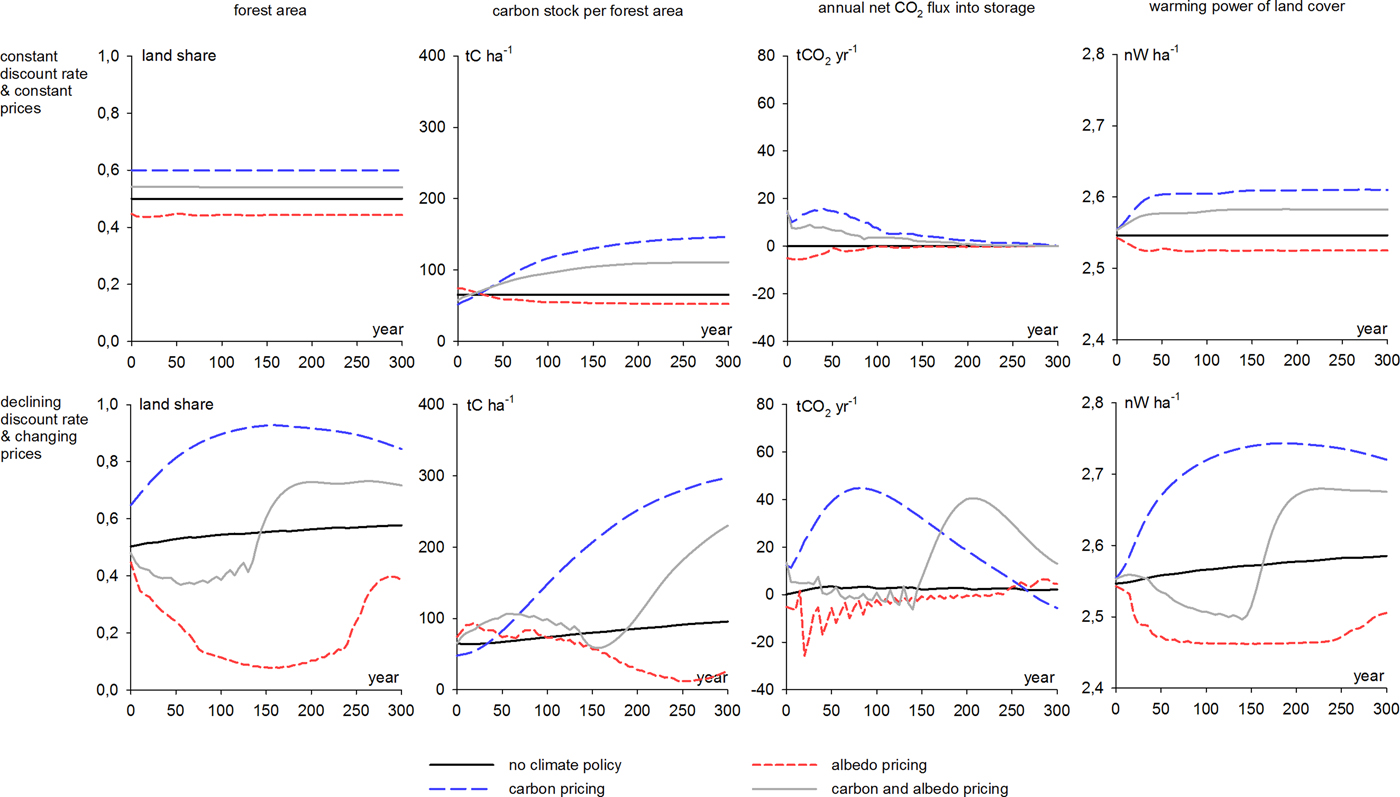
Figure 7. Development of forest area, carbon density (i.e., carbon stock per hectare), annual net CO2 flux into storage and the warming power of the landscape during the next 300 years (60 periods) with alternative climate policies and discounting schemes, when the growth description of a less productive site (in Northern Finland) is used to describe the stand growth instead of the growth description applied elsewhere in the study.
Sensitivity Analysis: Climate Policy Stringency
The SCC and SCF trajectories used to price carbon and albedo in this study are exogenous. SCC and SCF estimates depend on how future damages are estimated, valued and discounted. Global future damages are naturally subject to large uncertainties and, thus, damage estimates vary considerably (Tol Reference Tol2012). Likewise, discounting assumptions vary considerably between IAMs (see, e.g., Stern (Reference Stern2006) and Nordhaus (Reference Nordhaus2006)). Therefore, different IAMs (and the same IAMs with different assumptions) produce very different estimates. For instance, the United States Government commissioned SCC estimates produced using the FUND model are considerably lower than those produced using DICE (United States Government 2015). Using systematically lower SCC and SCF values in the calculations would imply a less stringent climate policy.
Another reason for considering the application of lower carbon and albedo prices is political. Climate policy is decreed politically and there may therefore be a discrepancy between “ideal” and actual climate policy. Thus, the prices applied in practice might not necessarily coincide with economists’ recommendations. Lower prices may be implemented as a political compromise between groups advocating different levels of climate policy stringency.
The impacts of less stringent policies to regulate carbon and albedo are illustrated in Figs. 8A and 8B. Expectedly, applying a less stringent climate policy leads to lesser deviations from the no-climate-policy baseline trajectories. Interestingly, regardless of climate policy stringency, timber harvests tend to follow a fairly similar trajectory for the first 50 years (after the initial adjustment).
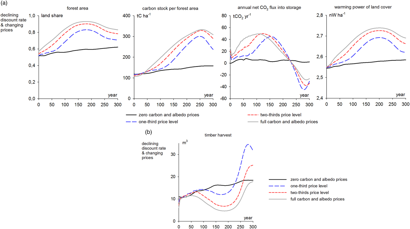
Figure 8. (A) Impact of climate policy stringency on forest area, carbon density (i.e., carbon stock per hectare), annual net CO2 flux into storage and the warming power of the landscape. The trajectories labelled “full carbon and albedo prices” were calculated with SCC and SCF values obtained from Rautiainen and Lintunen (2017). One-third price level and two-thirds price level reflect carbon and albedo prices equal to one-third and two-thirds of the SCC and SCF values, respectively. (B) Impact of climate policy stringency on timber harvests. The trajectories labelled full carbon and albedo prices were calculated with SCC and SCF values obtained from Rautiainen and Lintunen (2017). One-third price level and two-thirds price level reflect carbon and albedo prices equal to one-third and two-thirds of the SCC and SCF values, respectively.
Welfare Impacts
The welfare impacts of alternative climate policies are displayed in Table 1. All policies are compared to the no-climate-policy baseline. The value of the climatic impacts is calculated assuming that the shadow prices for carbon and albedo obtained from DICE depict the true social value of the climatic impacts, regardless of whether these impacts are regulated. The monetary values provided reported in Table 1 depict the net present values of costs and benefits accrued over the infinite time horizon.
Table 1. Welfare gains from alternative climate policies

Full carbon and albedo pricing, i.e., the policy regulating both externalities, generates the greatest welfare gains (856 €/ha). Also carbon pricing alone improves welfare (422 €/ha), but albedo pricing alone reduces it (−743 €/ha).
The greatest climate benefits (2389 €/ha) are obtained when carbon pricing is implemented alone. However, the same policy also leads to the greatest welfare losses in terms of food and timber production (−1946 €/ha). Complementing carbon pricing with albedo regulation reduces climate benefits (by 782 €/ha from 2389 €/ha to 1607 €/ha), but also reduces welfare losses from reduced food and timber production (by 1193 €/ha from-1946 €/ha to 752 €/ha). Thus, regulating also albedo increases welfare, as balancing the two opposing externalities leads to smaller losses in production.
Notable welfare gains can be achieved by regulating carbon and albedo even if the applied prices are lower than what would be socially optimal. Pricing carbon and albedo at one-third of their social value is already enough to produce 59 percent of the total achievable welfare gains (i.e., 507 €/ha out of 856 €/ha). Prices equal to two-thirds of their social value produce 91 percent of the gains (i.e., 778 €/ha out of 856 €/ha).
Also, notable welfare gains can be achieved even if the land use is fixed. In the present setup this means that the agricultural sector is not affected by the climate policy and welfare gains are obtained through changed forest management only.Footnote 27 Changing forest management alone can generate 63 percent of the total achievable welfare gains (i.e., 536 €/ha out of 856 €/ha). Interestingly, the welfare gains from carbon pricing alone are equally large regardless of whether land use is fixed or not. However, the composition of the welfare gains differs. When the land use is fixed, carbon pricing produces smaller climate benefits (as agricultural land cannot be afforested) but also smaller welfare losses in the production sector (as less food production is lost). Coincidentally, these two effects cancel out. The fixed land-use also constrains the welfare losses when only albedo is regulated.
Policy Implications
The Paris agreement aims at limiting the rise in global mean temperature to 1.5–2 °C beyond the preindustrial level. Reaching the target requires strong reductions in net CO2 emission in the short term and possibly net negative emissions during the latter half of the 21st century (Peters et al. Reference Peters, Andrew, Boden, Canadell, Ciais, Quéré and Wilson2012, Fuss et al. Reference Fuss, Canadell, Peters, Tavoni, Andrew, Ciais and Le Quéré2014, Anderson and Peters Reference Anderson and Peters2016). Technological solutions to produce negative emissions are currently expensive (Smith et al. Reference Smith, Davis, Creutzig, Fuss, Minx, Gabrielle and Van Vuuren2016). Using forest to remove CO2 from the atmosphere and increasing carbon storage in ecosystems and forest products has been proposed as a cheaper option. Increased carbon storage can be achieved by subsidizing it (see e.g., Lintunen and Uusivuori Reference Lintunen and Uusivuori2016). Recent studies from boreal forests in Norway and Finland suggest that substantial additional net removals in the forest sector could be obtained by implementing a CO2 price in the range of 20 to 30 €/tonne (Sjølie, Latta, and Solberg. Reference Sjølie, Latta and Solberg2013b, Pohjola et al. Reference Pohjola, Laturi, Lintunen and Uusivuori2018). However, the climatic impacts of albedo changes are not considered in these analyses. Taking albedo into account may alter the policies’ expected outcomes (Sjølie, Latta, and Solberg Reference Sjølie, Latta and Solberg2013a).
Based on our findings we make the following (tentative) policy recommendations regarding the implementation of forest carbon and albedo pricing in boreal regions.
(1) If forest carbon pricing is implemented in boreal conditions, it should be complemented by albedo pricing. Carbon pricing alone is not sufficient for regulating the climatic impacts of forestry. While it does increase welfare compared to the no-climate-policy option, complementing the policy with albedo pricing leads to notably larger welfare gains (Table 1). Carbon pricing leads to an overprovision of climate benefits at the expense of food and timber production. Complementing the policy with albedo pricing reduces these welfare losses, as it limits the afforestation of agricultural land and maintains harvests at a higher level (in the case of tightening climate policy).
(2) Albedo pricing alone (without carbon pricing) should be avoided. If carbon is not priced, albedo pricing may reduce welfare (Table 1).
(3) Jointly regulating carbon and albedo can have notable positive welfare effects, even if the applied carbon and albedo prices are lower than what would be socially optimal. Likewise, if the landscape share of forests is large enough, notable benefits can be obtained even if land use is held fixed, and only forest management is targeted by the policy.
(4) An effort should be made to reduce the uncertainty regarding the warming power of surface albedo. The strength of the albedo effect relative to the forests capacity to remove carbon from the atmosphere is crucial to determining how the trade-off between carbon and albedo should be taken into account in land use and forest management (Figs. 5 and 6). Regulating albedo based on a false appraisal of its warming impact may reduce the policy's welfare impacts.
(5) An effort should be made to measure and regulate other climate externalities. Most notably, the impact of aerosols emitted by forests is not considered in this study and may lead to further refinements in the policy recommendations. The importance of including missing externalities in the analysis is highlighted by the comparison of the carbon-only and the carbon-and-albedo policies considered in this study.
Limitations of This Study
This study has certain limitations which are largely a result of the simplifying assumptions made to reduce the complexity of the model. Below, we discuss them briefly. Naturally, each limitation is a challenge to future research.
First, the potential substitution of fossil fuels and materials by biomass is not taken into account in our model. The inverse demand functions for timber and crops are time-invariant. In reality, demand functions may change over time. Specifically, a tightening climate policy that encourages the substitution of non-renewables by renewables may shift the demands for crops and timber.
Second, the applied descriptions of tree growth, biomass decay and age-class albedo dynamics are time-invariant. However, climate change alters these processes, and thus affects forest management (see, e.g., Sohngen, Mendelsohn, and Sedjo Reference Sohngen, Mendelsohn and Sedjo2001, Hanewinkel et al. Reference Hanewinkel, Cullmann, Schelhaas, Nabuurs and Zimmermann2013). Warming accelerates tree growth, which increases annual carbon removals. Nevertheless, it also accelerates the decomposition of harvesting residues. Climate change shortens the duration of snow cover in many parts of the boreal region. As the albedo of the landscape is lower without snow, shorter winters make the landscape darker (on average over time), which increases the mean annual warming power of its surface and may also change the relative difference between the warming power of forests and treeless land. These changes are not taken into account in this study.
Third, we omit the land use impacts of other policies, besides climate policy. Other policies also affect land use decisions—at least in the short and medium termFootnote 28. For example, agricultural policies may improve the profitability of agriculture, and conservation policies may set restrictions on land use conversions. The details of these policies vary between countries. We neglect these policies, as we focus on the general properties of joint regulation.
Fourth, we assume that all land is homogenous. In reality, variable land quality may restrict land use conversions. In Nordic countries, for example, some (relatively unproductive) forests are located on land that is too marginal to be meaningfully used for productive agriculture. Thus, while all agricultural land might potentially be converted to forest, all forest land could not be converted to agriculture. Including more land uses, forest types and heterogeneous land quality in the model would diversify the potential to adapt land use to stricter climate policy. For instance, increasing the share of broadleaved forests, or broadleaved species in mixed forests, could be used to reduce the albedo effect of forests (Matthies and Valsta Reference Matthies and Valsta2016). Optimal forest management may vary between sites that are spatially close but differ in productivity (Lutz et al. Reference Lutz2016).
Conclusions
The market-level impacts of jointly regulating carbon and albedo differ from those of carbon regulation alone. Carbon pricing encourages afforestation and carbon storage, whereas albedo pricing encourages high albedo land-uses such as agriculture. Carbon pricing alone leads to an overprovision of climate benefits through excessive carbon sequestration at the expense of food and timber production. Complementing the policy with albedo pricing reduces these welfare losses while it balances welfare gains from carbon sequestration and higher albedo and, therefore, increases welfare. The impacts of carbon and albedo pricing are sensitive to variation in parameter values (albedo strength, productivity of forest land, and carbon and albedo prices). Thus, to be able to effectively implement carbon and albedo pricing, it is important to establish the strength of the albedo effect accurately. Inaccurate albedo pricing may cause unnecessary welfare losses.
Supplementary material
The supplementary material for this article can be found at https://doi.org/10.1017/age.2018.8
Appendix 1
The Lagrangian to the welfare maximization problem is
 $$\eqalign{L = & \mathop \sum \limits_{t = 0}^\infty B_{0t}\left[ {U\left( {\mathop \sum \limits_{a = 1}^\infty {\rm \sigma }_av_az_{at}} \right) + \tilde{U}(by_t)} \right. \cr &- p_t^w \left( {w_0x_t^0 + \mathop \sum \limits_{a = 1}^\infty w_a(x_{at} - z_{at}) + w_0y_t} \right) \cr & - \left( {c_h\mathop \sum \limits_{a = 1}^\infty v_az_{at} + {\tilde{c}}_hby_t + c_rx_t^0 + c_fy_t} \right) \cr &+ p_t^c \left[ \matrix{(\gamma _v + \gamma _b)\left[ {\mathop \sum \limits_{a = 1}^\infty (v_{a + 1} - v_a)x_{at} + v_1x_t^0 - \mathop \sum \limits_{a = 1}^\infty v_{a + 1}z_{at}} \right] \hfill \cr + (\gamma _v + \gamma _b)\mathop \sum \limits_{a = 1}^\infty v_az_{at} - \mathop \sum \limits_{a = 1}^\infty v_a\mathop \sum \limits_{\,j = 0}^\infty \left( {\gamma _v{\rm \delta }_j^P + \gamma _b{\rm \delta }_j^S } \right)z_{a,t - j} \hfill} \right] \cr & + \lambda _t^b \left( {y_{t - 1} + \; \mathop \sum \limits_{a = 1}^\infty z_{at} - y_t - x_t^0 } \right) + {\rm \beta }_t{\rm \lambda }_{1,t + 1}^f \left( {x_t^0 - x_{1,t + 1}} \right)\; \cr &+ \mathop \sum \limits_{a = 1}^\infty {\rm \beta }_t{\rm \lambda }_{a + 1,t + 1}^f (x_{at} - \; z_{at} - x_{a + 1,t + 1})\left.{ + \mathop \sum \limits_{a = 1}^\infty {\rm \mu }_{at}^{\bar z} (x_{at} - \; z_{at})} \right] } $$
where  $\lambda_{t} $ are Lagrangian multipliers. The Karush-Kuhn-Tucker conditions for an optimal solution are
 $$\eqalign{B_{0t}\displaystyle{{\partial L} \over {\partial x_t^0}} = & - c_r + p_t^c \lpar \gamma _v + \gamma _b\rpar v_1 - p_t^w w_0 - \lambda _t^b + \beta _t\lambda _{1\comma t + 1}^f \le 0\comma \; \cr & \; x_t^0 \ge 0\comma \; \; x_t^0 \displaystyle{{\partial L} \over {\partial x_t^0}} = 0\; \forall \; t \ge 1,}$$
 $$\eqalign{B_{0\comma t + 1}\displaystyle{{\partial L} \over {\partial x_{a\comma t + 1}}} \,= \,& p_{t + 1}^c \lpar \gamma _v + \gamma _b\rpar \lpar v_{a + 1} - v_a\rpar - p_{t + 1}^w w_a - \lambda _{a\comma t + 1}^f \cr & + \beta _{t + 1}\lambda _{a + 1\comma t + 2}^f + \mu _{a\comma t + 1}^{\bar z} \le 0\comma \; \cr & \; x_{a\comma t + 1} \ge 0\comma \; \; x_{a\comma t + 1}\displaystyle{{\partial L} \over {\partial x_{a\comma t + 1}}} = 0\; \forall \; t \ge 0\comma \; \; a \ge 1,}$$
 $$\eqalign{B_{0t}\displaystyle{{\partial L} \over {\partial z_{at}}} =\, & \lpar U^{\rm {\prime}}\lpar q_t\rpar \sigma _a - c_h\rpar v_a + p_t^w w_a - p_t^c \lpar v_{a + 1} - v_a\rpar \lpar \gamma _v + \gamma _b\rpar \cr & - v_a\mathop \sum \limits_{\,j = 0}^\infty B_{t\comma t + j}p_{t + j}^c \lpar{\gamma _v\delta _j^P + \gamma _b\delta _j^S} \rpar+ \lambda _t^b - \beta _t\lambda _{a + 1\comma t + 1}^f - \mu _{at}^{\bar z} \le 0\comma \; \cr & \; z_{at} \ge 0\comma \; \; z_{at}\displaystyle{{\partial L} \over {\partial z_{at}}} = 0\; \forall \; t \ge 1,}$$
 $$\eqalign{B_{0t}\displaystyle{{\partial L} \over {\partial y_t}} =\,& \lpar \tilde{U}^{\prime}\lpar \tilde{h}_t\rpar - \tilde{c}_h\rpar b - c_f - p_t^w w_0 - \lambda _t^b + \beta _t\lambda _{t + 1}^b \le 0 \comma \; \cr &y_t \ge 0\comma \; \; y_t\displaystyle{{\partial L} \over {\partial y_t}} = 0\; \forall \; t \ge 1,}$$
 $$\displaystyle{{\partial L} \over {\partial \lambda _t^a}} = 0\; \forall \; a\comma \; t\comma \; $$
 $$\displaystyle{{\partial L} \over {\partial \lambda _t^y}} = 0\; \forall \; t\comma $$
and
 $$\mu _{at}^{\bar z} \ge 0\comma \; \lpar x_{at} - \; z_{at}\rpar \ge 0\; \comma \; \; \mu _{at}^{\bar z} \lpar x_{at} - \; z_{at}\rpar = 0\; \forall \; a\comma \; t.$$
Appendix 2
At steady state, the inequalities (14) and (15) hold as equations and  $\mu _a^{\bar z} \; = 0\; \forall \; a \le a^*$. Substituting the expression for λ f1 [from (15)] into (14), and then similarly recursively substituting λ f2, …, λ fa*, we obtain
 $$- c_r + \mathop \sum \limits_{a = 0}^{a^{\ast} - 1} \beta ^a \left[ p^c\lpar \gamma _v + \gamma _b\rpar \lpar v_{a + 1} - v_a\rpar - p^ww_a \right] \; + \beta ^{a^{\ast}}\lambda ^f_{a^{\ast}} = \lambda ^b.$$
From (15) we obtain an expression for λ a*, i.e.,
 $$\lambda ^f_{a^{\ast}} = U^{\rm {\prime}}\lpar q\rpar \sigma _av_a - c_hv_a - h\lpar{\gamma _b\mathop \sum \limits_{\,j = 1}^n \beta ^jp^c\delta _j^S + \gamma _v\mathop \sum \limits_{k = 1}^m \beta ^kp^c\delta _k^P} \rpar+ \lambda ^b\comma$$
where q = σ a*v a*z a* = σ a*v a*x a*, because an unique optimal rotation is assumed. Substituting λ fa* from (A10) into (A9) and rearranging, we obtain (18).


 Open access