


Introduction
The American bison is a charismatic mammal that is used to be a vital symbol and resource for Native Americans and helped shape grassland landscapes across North America. However, the American government and commercial interests nearly drove the bison to extinction in the late ${19^{th}}$
century through over-hunting and habitat destruction (Taylor Reference Taylor2011). Government agencies and non-profit conservation groups are now restoring prairies and reintroducing bison to their historical range in an ongoing effort to bring this iconic mammal back from the brink of extinction in the wild (Zumbach Reference Zumbach2015). However, the net economic impact of bison reintroduction on rural communities has not been studied (Emmet Jones et al. Reference Emmet Jones, Mark Fly, Talley and Ken Cordell2003). This paper informs debate over the likely economic effects of bison reintroduction with a nationwide assessment of the local economic impacts of bison reintroduction. We estimate the causal impacts of bison herd establishment on county-level income, employment, and population growth so that rural communities can take economic well-being into account when considering their future decisions regarding bison restoration.
${19^{th}}$
century through over-hunting and habitat destruction (Taylor Reference Taylor2011). Government agencies and non-profit conservation groups are now restoring prairies and reintroducing bison to their historical range in an ongoing effort to bring this iconic mammal back from the brink of extinction in the wild (Zumbach Reference Zumbach2015). However, the net economic impact of bison reintroduction on rural communities has not been studied (Emmet Jones et al. Reference Emmet Jones, Mark Fly, Talley and Ken Cordell2003). This paper informs debate over the likely economic effects of bison reintroduction with a nationwide assessment of the local economic impacts of bison reintroduction. We estimate the causal impacts of bison herd establishment on county-level income, employment, and population growth so that rural communities can take economic well-being into account when considering their future decisions regarding bison restoration.
Currently, fifty-three bison herds exist in the U.S. These herds could have a range of effects on the people around then. Bison reintroduction could increase the attachment people have to grassland areas (Wilkins et al. Reference Wilkins, Pejchar and Garvoille2019) and might improve the health of rural economies by increasing local tourism through wildlife marketing (Vasile Reference Vasile2018). However, farmers, ranchers, and local residents have expressed concerns regarding bison reintroduction. For example, the presence of bison could limit profitable use of cropland and rangeland re-purposed as bison habitat. Cattle ranchers worry about the potential for diseases like brucellosis to spread from bison to cattle, and rural leaders worry that bison establishment could be a step on the path to national monument designation, which might limit economic activity (Boyd and Gates Reference Boyd and Gates2006; Davenport Reference Davenport2018).
Economists have studied several dimensions of the relationship between conservation and local economies. One body of research on the effects of protecting nature on local economic activity has focused on land conservation. Some studies raised concern that protected areas could be a threat to local economic well-being (Rasker Reference Rasker1993) and that rapid growth in nature-based visitation could challenge local community resilience (Winter et al. Reference Winter, Selin, Cerveny and Bricker2020). However, other papers have suggested that protected areas can improve conditions in local economies. Increased tourism can in some cases provide more employment opportunities (Andam et al. Reference Andam, Ferraro, Pfaff, Sanchez-Azofeifa and Robalino2008, Reference Andam, Ferraro, Sims, Healy and Holland2010; Albers and Robinson Reference Albers and Robinson2013; Bode et al. Reference Bode, Tulloch, Mills, Venter and Ando2015), increase income (Wunder Reference Wunder2000), and promote local business establishment and economic development (Walls et al. Reference Walls, Lee and Ashenfarb2020). Work by Kennedy et al. (Reference Kennedy, Miteva, Baumgarten, Hawthorne, Sochi, Polasky, Oakleaf, Uhlhorn and Kiesecker2016) showed that the economic effects of conservation depend critically on the scale and nature of the interventions, and other papers found that land conservation, as in the northern forest region of the U.S. (Lewis et al. Reference Lewis, Hunt and Plantinga2002) or new large national monuments (Jakus and Akhundjanov Reference Jakus and Akhundjanov2019), has had no significant effects on local economies at all.
A body of work has also studied the local economic effects of wildlife conservation and restoration itself, with similarly mixed findings Langpap et al. Reference Langpap, Kerkvliet and Shogren2020). Some papers showed that species conservation has negative effects on measure of local economic health like income, population, or employment (Lewis et al. Reference Lewis, Kaweche and Mwenya1990; Emerton Reference Emerton2001; Eichman et al. Reference Eichman, Hunt, Kerkvliet and Plantinga2010; Ferris and Frank Reference Ferris and Frank2021). However, others found that species conservation can actually improve some dimensions of local economic activity and human well-being (Fernandez et al. Reference Fernandez, Richardson, Tschirley and Tembo2009; Chen et al. Reference Chen, Lewis and Weber2016; Raynor et al. Reference Raynor, Grainger and Parker2021).
Thus, previous research on the economic effects of wildlife conservation or restoration does not yield clear predictions for the likely impact of bison reintroduction in the U.S. In a hypothetical choice experiment study, Foelske et al. (Reference Foelske, Van Riper, Stewart, Ando, Gobster and Hunt2019) found that residents near bison herds in Illinois and Iowa actually had no preference for those herds either to grow or shrink in future scenarios of their communities. Research on other charismatic species implies bison reintroduction might drive increases in visitor expenditures and help local economies (Wilson and Tisdell Reference Wilson and Tisdell2003; Loomis and Caughlan Reference Loomis and Caughlan2004; Duffield et al. Reference Duffield, Neher and Patterson2008). On the other hand, cattle ranchers have persistent fears that bison may reduce incomes by competing for rangeland with cattle, even though experimental research does not show that to be the case (Kohl et al. Reference Kohl, Krausman, Kunkel and Williams2013). There has been no study of how bison reintroduction in grassland areas actually affects local economic well-being in the U.S. to show whether positive or negative effects have actually come to pass. This paper fills that gap.
We assemble a novel data set that includes information on each herd’s name, location, type, size, and year of establishment for all 53 bison herds in the U.S. There are 66 counties in 19 states in the U.S. that have bison herds established between 1860 and 2018. We merge county-level data from the U.S. Bureau of Economic Analysis (BEA) on economic health with the data on bison herds to study the impact of bison reintroduction on local economic development in the counties that host them.
A simple probit model shows the presence of bison herds in a county and is positively correlated with the county’s per capita income. However, that correlation should not be interpreted as a causal link between bison and economic activity since bison are not randomly placed in the landscape, and many other factors could influence local economies. Thus, we use other methods – staggered difference-in-difference (DID) with multiple time periods and the synthetic control method (SCM) – to estimate the causal impact of bison reintroduction on local employment, population, and per capita income.
Similar to the results of Jakus and Akhundjanov (Reference Jakus and Akhundjanov2019) described above, our causal inference analyses find little evidence of any significant impact of bison reintroduction on local economic activity, either positive or negative. Results from our DID analysis show that bison reintroduction has no significant impact on per capita income, the total number of jobs, or population density. Results from the SCM are consistent with the findings of the DID analysis; bison reintroduction has an insignificant impact on local economic health. Thus, the results of this study suggest that while bison reintroduction may not be a big local economic driver, it also does not undermine local economic health.
Empirical strategy
One could readily estimate the average treatment effect attributable to bison reintroduction if bison herds were randomly established in U.S. counties. However, since bison reintroduction happened in selective locations, it is challenging to identify the causal relationship between bison reintroduction and the local economy. This section presents the two causal inference methods we use to estimate the impact of bison reintroduction on local economic health: staggered DID and SCM.
DID with multiple time periods
Bison herds were established in different years across the landscape; thus, we adopt a staggered DID design with multiple treatment periods. A two-way fixed effects (TWFE) model is commonly applied in these circumstances. However, recent research documents potential shortcomings of this specification (Borusyak and Jaravel Reference Borusyak and Jaravel2017; Callaway and Sant’Anna Reference Callaway and Sant’Anna2021; De Chaisemartin and d’Haultfoeuille Reference De Chaisemartin and d’Haultfoeuille2020; Goodman-Bacon Reference Goodman-Bacon2021) More specifically, a TWFE model with multiple treatment timing not only compares the newly treated county with never treated and not-yet treated counties but also compares newly treated counties with already treated units. The last comparison may bias the estimated treatment effect since the path of outcomes for already treated units includes treatment effect dynamics and cannot serve as a good control (Callaway and Sant’Anna Reference Callaway and Sant’Anna2021). To address this issue, we follow an alternative approach proposed by Callaway and Sant’Anna (Reference Callaway and Sant’Anna2021), which only uses the desirable comparisons instead of all possible comparisons to estimate treatment effects.
Callaway and Sant’Anna (Reference Callaway and Sant’Anna2021) first calculate the group-time average treatment effects $ATT(g,t)$
, which is a unique ATT for a cohort of units treated at the same point in time. The group-time average treatment effects are estimated as follows:
$ATT(g,t)$
, which is a unique ATT for a cohort of units treated at the same point in time. The group-time average treatment effects are estimated as follows:
 $$ATT(g,t) = E[{Y_t}(g) - {Y_t}(0)|G = g]$$
where G is the time period when a county has bison herds established. Treatment counties are grouped based on the establishment years of bison herds. Once a county establishes a bison herd, it remains treated (staggered treatment adoption assumption). We restrict the control group to be the group of counties that have not yet participated in the treatment in that time period, including all never-treated counties and additional counties that eventually establish bison herds but have not yet established.
Bison counties may be comparable to non-bison counties conditioning on observed pre-treatment covariates, X. We use these covariates to predict the conditional probability of being treated (have bison herds established). Observed pre-treatment covariates included in the analysis are county size, average precipitation, mean temperature, elevation, the percentage of land that are grasslands and shrubs in 2001, and whether the county is in a metropolitan area. Footnote 1 After conditioning on observed pre-treatment covariates, the conditional parallel trend assumption based on not-yet been treated units is given as follows.
For all g = 2, …G; s,t = 2,., $\tau $
with
$\tau $
with $t \ge g$
and
$t \ge g$
and $s \ge t$
 $$E[{Y_t}(0) - {Y_{t - 1}}(0)|X,G = g] = E[{Y_t}(0) - {Y_{t - 1}}(0)|X,{D_s} = 0,G \ne g]$$
Under this parallel trend assumption, we can use the not-yet-treated by time s ( $s \ge t$
) units as control groups when calculating the effect for the group that is first treated in time g. We estimate the group-time average treatment effects through doubly robust (DR) estimation procedure recommended by Callaway and Sant’Anna (Reference Callaway and Sant’Anna2021) and Sant’Anna and Zhao (Reference Sant’Anna and Zhao2020). The DR estimation combines outcome regression (OR) proposed by Heckman et al. (Reference Heckman, Ichimura and Todd1997) and inverse probability weighting (IPW) estimators proposed by Abadie (Reference Abadie2005) into one specification. The DR estimators share the strengths of OR and IPW because they can identify the ATT even if one of the two models (the propensity score model and the OR model) is misspecified (Sant’Anna and Zhao Reference Sant’Anna and Zhao2020).
$s \ge t$
) units as control groups when calculating the effect for the group that is first treated in time g. We estimate the group-time average treatment effects through doubly robust (DR) estimation procedure recommended by Callaway and Sant’Anna (Reference Callaway and Sant’Anna2021) and Sant’Anna and Zhao (Reference Sant’Anna and Zhao2020). The DR estimation combines outcome regression (OR) proposed by Heckman et al. (Reference Heckman, Ichimura and Todd1997) and inverse probability weighting (IPW) estimators proposed by Abadie (Reference Abadie2005) into one specification. The DR estimators share the strengths of OR and IPW because they can identify the ATT even if one of the two models (the propensity score model and the OR model) is misspecified (Sant’Anna and Zhao Reference Sant’Anna and Zhao2020).
After calculating $ATT(g,t)$
, we follow Callaway and Sant’Anna (Reference Callaway and Sant’Anna2021)’s recommendation to summarize all feasible
$ATT(g,t)$
, we follow Callaway and Sant’Anna (Reference Callaway and Sant’Anna2021)’s recommendation to summarize all feasible $ATT(g,t)$
into an overall effect parameter. Since we only have a limited number of bison herds established in each time period, the group size is small in our analysis. Statistical inference on group-time average treatment may become tenuous with small groups (Callaway and Sant’Anna Reference Callaway and Sant’Anna2021). Thus, we aggregate treatment effects of bison reintroduction on local economic outcomes by averaging all of the identified group-time average treatment effects with weights proportional to group size. In this case, the effective sample size is the total number of units that have ever been treated, and the statistical inference results can be more stable. The overall effects of bison reintroduction on income per capita, jobs, and population density across all groups that have ever had bison herds established are discussed in “Difference-in-difference (DID) with multiple time periods.” To examine if the conditional parallel trend assumption is satisfied, we aggregate the group-time average treatment effects to an event study plot to show the average treatment effects at different lengths of exposure to the treatment. The parallel trend assumption holds if the average effects are not significantly different from zero in the pre-treatment periods (Callaway and Sant’Anna Reference Callaway and Sant’Anna2021).
$ATT(g,t)$
into an overall effect parameter. Since we only have a limited number of bison herds established in each time period, the group size is small in our analysis. Statistical inference on group-time average treatment may become tenuous with small groups (Callaway and Sant’Anna Reference Callaway and Sant’Anna2021). Thus, we aggregate treatment effects of bison reintroduction on local economic outcomes by averaging all of the identified group-time average treatment effects with weights proportional to group size. In this case, the effective sample size is the total number of units that have ever been treated, and the statistical inference results can be more stable. The overall effects of bison reintroduction on income per capita, jobs, and population density across all groups that have ever had bison herds established are discussed in “Difference-in-difference (DID) with multiple time periods.” To examine if the conditional parallel trend assumption is satisfied, we aggregate the group-time average treatment effects to an event study plot to show the average treatment effects at different lengths of exposure to the treatment. The parallel trend assumption holds if the average effects are not significantly different from zero in the pre-treatment periods (Callaway and Sant’Anna Reference Callaway and Sant’Anna2021).
SCM
The SCM uses a data-driven approach to construct a synthetic unit that closely matches each of the treated counties in pre-treatment periods. In contrast to the DID, the SCM allows for the effects of time-varying unobserved factors (Kreif et al. Reference Kreif, Grieve, Hangartner, Turner, Nikolova and Sutton2016). This synthetic unit is a weighted average of several untreated counties, where the weights are determined in the pre-treatment periods regarding how closely the control units match the treated county. We use this synthetic unit as the counterfactual for the treated county in post-treatment periods to assess the effects of bison reintroduction on local economic development (Abadie and Gardeazabal Reference Abadie and Gardeazabal2003; Abadie et al. Reference Abadie, Diamond and Hainmueller2010; Abadie et al. Reference Abadie, Diamond and Hainmueller2015). As a small-sample comparative case study approach, this method also provides more informative results on how bison reintroduction affects each treated county’s local economy and the effects on outcome variables during each post-treatment period.
We use the SCM to examine the treatment effects of bison reintroduction on local economic development. We estimate the county-specific effects of bison reintroduction and the average effects across each county with bison herds. In the following paragraphs, we first discuss how we follow Abadie et al. (Reference Abadie, Diamond and Hainmueller2010, Reference Abadie, Diamond and Hainmueller2015) and conduct the SCM for each single treated county. Then, we explain how to generalize this SCM for multiple treated units following Cavallo et al. (Reference Cavallo, Galiani, Noy and Pantano2013).
For a single county with bison reintroduction, suppose we have J + 1 counties observed for T time periods, and only the first county has bison herds, while the remaining J counties are considered potential controls (donors). Suppose time periods 1 to ${T_0}$
are the pre-treatment periods and
${T_0}$
are the pre-treatment periods and ${T_0} + 1$
to T are the post-treatment periods, the bison reintroduction occurs at
${T_0} + 1$
to T are the post-treatment periods, the bison reintroduction occurs at ${T_0} + 1$
. Let
${T_0} + 1$
. Let $Y_{jt}^N$
be a vector of outcome variables that would be observed for county j at time t in the absence of treatment and
$Y_{jt}^N$
be a vector of outcome variables that would be observed for county j at time t in the absence of treatment and $Y_{jt}^J$
be the observed outcome if j is treated in the periods
$Y_{jt}^J$
be the observed outcome if j is treated in the periods ${T_0} + 1$
to T. Assuming bison reintroduction did not affect the bison county in the pre-treatment periods, we have
${T_0} + 1$
to T. Assuming bison reintroduction did not affect the bison county in the pre-treatment periods, we have $Y_{jt}^N = Y_{jt}^J$
for all j in 1, …–N during t in 1, …,
$Y_{jt}^N = Y_{jt}^J$
for all j in 1, …–N during t in 1, …, ${T_0}$
.
${T_0}$
.
Let ${\alpha _{jt}} = Y_{jt}^J - Y_{jt}^N$
represents the effect of bison reintroduction for county j at time t. Given that only the first county is treated after
${\alpha _{jt}} = Y_{jt}^J - Y_{jt}^N$
represents the effect of bison reintroduction for county j at time t. Given that only the first county is treated after ${T_0} + 1$
, we aim to estimate,
${T_0} + 1$
, we aim to estimate, ${\alpha _{1t}}$
, during the post-treatment periods (
${\alpha _{1t}}$
, during the post-treatment periods ( $t \gt {T_0}$
). As shown in Equation 3,
$t \gt {T_0}$
). As shown in Equation 3, ${\alpha _{1t}}$
can be written as:
${\alpha _{1t}}$
can be written as:
 $${\alpha _{1t}} = Y_{1t}^J - Y_{1t}^N$$
Given that $Y_{1t}^J$
is observed, we find
$Y_{1t}^J$
is observed, we find ${\alpha _{1t}}$
by estimating
${\alpha _{1t}}$
by estimating $Y_{1t}^N$
with the SCM and replacing the unobserved
$Y_{1t}^N$
with the SCM and replacing the unobserved $Y_{1t}^N$
in Equation 3 with a synthetic counterfactual outcome.
$Y_{1t}^N$
in Equation 3 with a synthetic counterfactual outcome. $Y_{1t}^N$
can be estimated by applying a reduced-form model given by Abadie et al. (Reference Abadie, Diamond and Hainmueller2010):
$Y_{1t}^N$
can be estimated by applying a reduced-form model given by Abadie et al. (Reference Abadie, Diamond and Hainmueller2010):
 $$Y_{jt}^N = {\sigma _t} + {\theta _t}{Z_j} + {\lambda _t}{\mu _j} + {\varepsilon _{jt}}$$
where ${\sigma _t}$
is the unknown time constant factor on
${\sigma _t}$
is the unknown time constant factor on $Y_{jt}^N$
across counties;
$Y_{jt}^N$
across counties; ${Z_j}$
is a vector of observed covariates that are affected by bison reintroduction and used as the predictors of the outcome variables;
${Z_j}$
is a vector of observed covariates that are affected by bison reintroduction and used as the predictors of the outcome variables; ${\mu _j}$
is the unobserved determinants of Y with its effect
${\mu _j}$
is the unobserved determinants of Y with its effect ${\lambda _t}$
allowing to vary over time; and the error terms
${\lambda _t}$
allowing to vary over time; and the error terms ${\varepsilon _{jt}}$
are unobserved factors with zero mean.
${\varepsilon _{jt}}$
are unobserved factors with zero mean. $Y_{1t}^N$
is estimated by using a weighted average of the outcome
$Y_{1t}^N$
is estimated by using a weighted average of the outcome $Y_{jt}^N$
of the donors. Thus,
$Y_{jt}^N$
of the donors. Thus,
 $$\hat Y_{1t}^N = \sum\limits_{j = 2}^{J + 1} {w_j}{Y_{jt}} = {\sigma _t} + {\theta _t}\sum\limits_{j = 2}^{J + 1} {w_j}{Z_j} + {\lambda _t}\sum\limits_{j = 2}^{J + 1} {w_j}{\mu _j} + \sum\limits_{j = 2}^{J + 1} {w_j}{\varepsilon _{jt}}$$
where $W = ({w_2}, \ldots ,{w_{J + 1}})$
is a vector of weights for the donors in the donor pool such that
$W = ({w_2}, \ldots ,{w_{J + 1}})$
is a vector of weights for the donors in the donor pool such that ${w_j} \ge 0$
for
${w_j} \ge 0$
for $j = 2, \ldots ,J + 1$
and
$j = 2, \ldots ,J + 1$
and ${w_2} + \ldots + {w_{J + 1}} = 1$
. Each particular value of the vector W defines a potential synthetic control.
${w_2} + \ldots + {w_{J + 1}} = 1$
. Each particular value of the vector W defines a potential synthetic control.
Assume that there exists a set of weights $W^{*} = ({w_2}, \ldots ,{w_{J + 1}})$
such that
$W^{*} = ({w_2}, \ldots ,{w_{J + 1}})$
such that
 $$\sum\limits_{j = 2}^{J + 1} w_j^*{Y_{jt}} = {Y_{1t}}\;fortin(1, \ldots ,{T_0})\;\;\;\;and\;\;\;\;\sum\limits_{j = 2}^{J + 1} w_j^*{Z_{jt}} = {Z_1}$$
then as proved by Abadie et al. (Reference Abadie, Diamond and Hainmueller2010), $\hat Y_{1t}^N$
will be an unbiased estimator of
$\hat Y_{1t}^N$
will be an unbiased estimator of $Y_{1t}^N$
and
$Y_{1t}^N$
and ${\alpha _{1t}}$
can be estimated using
${\alpha _{1t}}$
can be estimated using
 $${\hat \alpha _{1t}} = {Y_{1t}} - \sum\limits_{j = 2}^{J + 1} {w_j}{Y_{jt}}$$
Using W* produces a weighted average of the available control units such that it closely mimics the treated county in terms of outcomes during the pre-intervention periods. W* is chosen to minimize the difference between the characteristics of the treated and synthetic control counties (Abadie et al. Reference Abadie, Diamond and Hainmueller2010). The root means squared prediction error (RMSPE) in the pre-treatment periods can be used to measure the goodness of fit of a synthetic county (Abadie et al. Reference Abadie, Diamond and Hainmueller2015). A large RMSPE signals a bad fit, which may increase inference uncertainty in the post-treatment periods.
We select non-bison counties into a donor pool and construct a synthetic county for a treated unit as a weighted average of the units in the donor pool. Selecting donors before implementing SCM narrows the difference between the treated and donor units regarding the observed characteristics and reduces the potential interpolation bias. It also reduces the donor pool’s size, saving computing time for the SCM estimation and avoiding overfitting (Abadie et al. Reference Abadie, Diamond and Hainmueller2010, Reference Abadie, Diamond and Hainmueller2015). We use propensity score nearest neighbor matching (one to thirty) to select non-bison counties as potential controls in the donor pool for wild and non-wild bison counties, respectively. Footnote 2, Footnote 3 Propensity scores are calculated using data on observed county geographical and socioeconomic characteristics – the same sets of covariates used in the DID approach.
Predictors used in the synthetic control estimation process include annual precipitation, annual temperature, and lagged outcome variables in pre-treatment periods. Both precipitation and temperature are averaged over the pre-treatment period when used as predictors. Kaul et al. (Reference Kaul, Klößner, Pfeifer and Schieler2015) point out that including all pre-treatment outcomes as separate predictors could bias the estimation. Therefore, only the lagged values of outcomes in the last five periods before the treatment year are included as separate predictors. The rest of the pre-treatment outcome lags are averaged when entering as a predictor.
We use a placebo test to determine the statistical significance of the estimated impacts of bison reintroduction (Abadie and Gardeazabal Reference Abadie and Gardeazabal2003; Abadie et al. Reference Abadie, Diamond and Hainmueller2010). For each treated county, we assign the same bison herd establishment year as a placebo to its donors in the donor pool and apply the SCM to every donor in our sample. Then, we examine if the estimated effect of a real bison reintroduction is large relative to the “treatment” effects produced by multiple placebo units in the donor pool. We can compute a lead-specific significance level (p-value) in the post-treatment period for the estimated impact as:
 $$p - value = Pr(\hat \alpha _{1,l}^{PL} > {\hat \alpha ^{1,l}}) = {{\sum\limits_{j = 2}^{J + 1} I (\hat \alpha _{1,l}^{PL(j)} > {{\hat \alpha }^{1,l}})} \over {\# of\;control\;counties\;in\;the\;door\;pool}}$$
where $\hat \alpha _{1,l}^{PL(j)}$
is the lead l-specific effect of bison reintroduction when a donor county j is assumed to have bison herd established at the same time as county
$\hat \alpha _{1,l}^{PL(j)}$
is the lead l-specific effect of bison reintroduction when a donor county j is assumed to have bison herd established at the same time as county $1$
. We use the p-value to assess how the estimate
$1$
. We use the p-value to assess how the estimate ${\hat \alpha _{1,l}}$
ranks in the distribution of placebo effects.
${\hat \alpha _{1,l}}$
ranks in the distribution of placebo effects.
Given the lead-specific estimates for one treated county is ( ${\hat \alpha _{1,{T_{0 + 1}}}}, \ldots ,{\hat \alpha _{1,T}}$
), we generalize the SCM to allow G counties to experience treatment at different times. The average effect over all the treatments is calculated as:
${\hat \alpha _{1,{T_{0 + 1}}}}, \ldots ,{\hat \alpha _{1,T}}$
), we generalize the SCM to allow G counties to experience treatment at different times. The average effect over all the treatments is calculated as:
 $$\bar \alpha = {1 \over G}\sum\limits_{g = 1}^G {({{\hat \alpha }_{g,{T_{0 + 1}}}} \ldots ,{{\hat \alpha }_{g,T}})} ,$$
To conduct statistical inference for $\bar \alpha $
, we construct a set of placebos
$\bar \alpha $
, we construct a set of placebos ${\bar \alpha ^{PL}}$
with which
${\bar \alpha ^{PL}}$
with which $\bar \alpha $
is compared for inference. We first compute all the placebo effects for each treated county, and then, we compute every possible placebo average effect at each lead. All the possible placebo averages are indexed by
$\bar \alpha $
is compared for inference. We first compute all the placebo effects for each treated county, and then, we compute every possible placebo average effect at each lead. All the possible placebo averages are indexed by $np = 1, \ldots ,{N_{\bar PL}}$
. Each placebo average is calculated by picking a single placebo estimate corresponding to each treated county g and then taking the average across all G placebos. We rank the actual lead-specific average treatment effect in the distribution of average placebo effects and compute the lead-specific p-value for the average effect of bison reintroduction. The p-value shows the proportion of average placebo effects that are at least as large as the average treatment effect.
$np = 1, \ldots ,{N_{\bar PL}}$
. Each placebo average is calculated by picking a single placebo estimate corresponding to each treated county g and then taking the average across all G placebos. We rank the actual lead-specific average treatment effect in the distribution of average placebo effects and compute the lead-specific p-value for the average effect of bison reintroduction. The p-value shows the proportion of average placebo effects that are at least as large as the average treatment effect.
 $$p - value_l = \frac{\sum^{N\bar{P}Lnp\,=\,1}I(\alpha_{l}^{P\bar{L}(np)} > \bar{\alpha}_l)}{N_{\bar{P}L}} $$
Data
This study uses three types of data constructed annually at the county level from 1969 to 2018: bison herd locations and characteristics, county-level economic measures, and physical characteristics of the land and climate. Table 1 shows the sources of variables used in the analysis. Data on outcome variables – per capita income, population, and the total number of jobs – come from the BEA. Data on county characteristics – temperature, precipitation, elevation, presence of grassland, and non-rural status – come from PRISM Climate Data, the National Map from U.S. Geological Survey Footnote 4 , the National Land Cover Database (NLCD), and the BEA. The percentage of land within a county that is grassland or shrubs is calculated by overlaying a shapefile that contains counties’ boundaries on raster data on national land cover from NLCD.
Table 1. Variables and data source

IUCN: International Union for Conservation of Nature; DOI: U.S. Department of the Interior National Park Service Report; APR: American Prairie Reserve Report.
Information on bison herds is gathered from International Union for Conservation of Nature (IUCN), U.S. Department of the Interior National Park Service (DOI 2014), American Prairie Reserve Report (APR 2017), and Davenport (Reference Davenport2018). Table A1 in the Appendix lists the establishment year and county locations of all the bison herds. Our data include fifty-three bison herds (including both wild and non-wild herds) established before 2018. Wild bison herds exist with limited or no human intervention; they range widely and serve authentic functions in their grassland habitats. In contrast, non-wild bison herds are fenced in and managed with veterinary care, providing value in display, research, and education. For example, the bison herd in Yellowstone is wild, while the Midewin National Tallgrass Prairie in Illinois hosts a display herd a short drive from Chicago.
Collectively, 66 counties in the U.S. have bison herds established. The maps in Figures 1, 2, and 3 visualize spatial patterns in the locations of those herds and local economic conditions by county. We use simple cross-sectional probit analysis to quantify those patterns and identify what types of counties are more likely to have restored bison herds (Table 2). The existence of non-wild bison herds is not significantly correlated with geographical or economic characteristics except elevation. The presence of wild herds is positively correlated with income and negatively correlated with population density if we only consider the socioeconomic variables. However, correlations between geography and socioeconomic characteristics mean those results disappear when geographic features are included. It seems wild bison herds are more likely to be established in cold areas with low precipitation and broad coverage by grasslands and shrubs.

Figure 1. Distribution of bison herds and income per capita in the U.S.

Figure 2. Distribution of bison herds and population density in the U.S.

Figure 3. Distribution of bison herds and unemployment rate in the U.S.
Table 2. Probit regression results
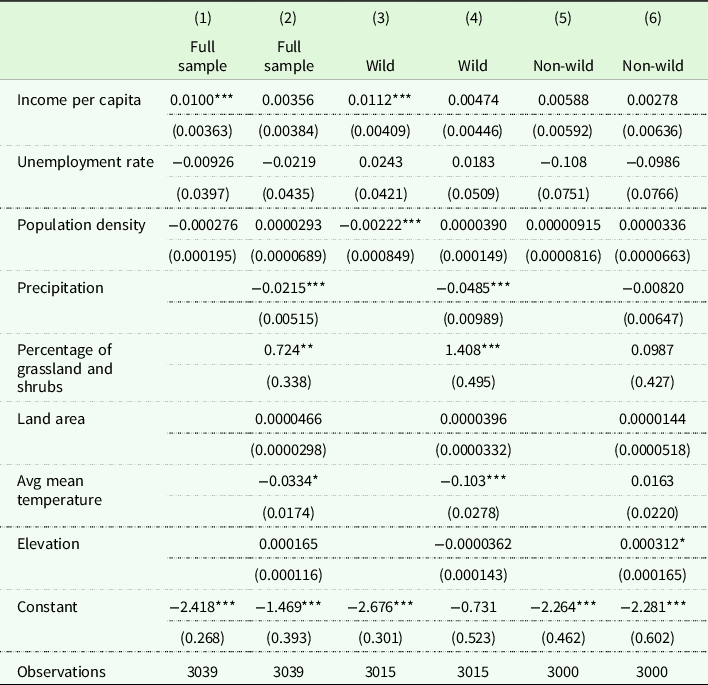
Standard errors in parentheses.
* p < 0.10.
** p < 0.05.
*** p < 0.01.
Note: Table 2 summarizes the results of cross-sectional probit analyses. Results in Column (1) and (2) show whether a county has a bison herd in 2018 as a function of its characteristics. The dependent variable in Column (3) and (4) is a binary variable indicating if a county has a wild bison herd, while the dependent variable in Column (5) and (6) is a binary variable indicating if a county has non-wild bison herd.
Given that data for outcome variables are only available from the year 1969 to 2018, we can only conduct the DID analysis using a sub-sample of the treatment units. We select 30 counties with bison herds that were established between 1970 and 2018 as the treatment group.
Implementing SCM places more demands on the data for pre-and post-treatment information. Given that data on the outcomes and covariates data are available from 1969 to 2018, we select 14 bison herds established between the year 1980 and 2005 for the treatment sample in the SCM analyses. These 14 bison herds in 16 counties provide a representative mix of wild and non-wild bison herds in the Midwest and West regions. Footnote 5
Results
In this section, we report the estimated impacts of bison reintroduction on population density, per capita income, and total local employment using the DID and SCM approaches.
DID with multiple time periods
Table 3 shows the effects of bison reintroduction on income per capita, population density, and the total number of jobs using the DID with DR estimation procedure. All outcomes are log-transformed, and standard errors are computed using the multiplier bootstrap. Point-estimate results imply that bison reintroduction reduces income per capita by 0.35%, population density by 2.41%, and the total number of jobs by 2.87%. However, all these effects on local economic development are insignificant. We also conduct the staggered DID using a pre-matched sample constructed by the propensity score matching (PSM). A detailed discussion of the DID with PSM results is available in Appendix B.
Table 3. The effect of bison reintroduction: DID with doubly robust estimator
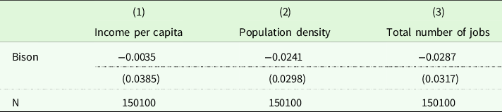
Standard errors in parentheses.
Note: This table summarizes the effects of bison reintroduction on income per capita, the total number of jobs, and population density using DID with the doubly robust DID estimators. We include 30 counties with bison herds established between 1970 and 2018 in the treatment group to conduct the staggered DID analysis with multiple treatment periods.
We graphically identify whether the conditional parallel trend assumption is satisfied using Figures 4, 5, and 6. These three figures present the average treatment effects of bison reintroduction at different lengths of exposure to treatment (similar to an event study plot) for the outcome variables income per capita, population density, and total number of jobs, respectively. Year zero represents the time period that a bison herd was established. The estimated coefficients show the average effects of bison reintroduction on a lag or lead before and after herds were established. The average effects are not significantly different from zero before herd establishments, implying that the conditional parallel trend assumption holds.

Figure 4. Average effect on income per capita by years after herd establishment.
Note: This figure shows the average effects on income per capita across the different exposure lengths to the treatment. Results are estimated using DID with DR estimation procedure. Year 0 represents the time period that a bison herd was established. The average effects are not significantly different from 0 before herd establishment, implying that the parallel assumption is satisfied.

Figure 5. Average effect on the total number of jobs by years after herd establishment.
Note: This figure shows the average effects on the total number of jobs across the different exposure lengths to the treatment. Results are estimated using DID with DR estimation procedure. Year 0 represents the time period that a bison herd was established. The average effects are not significantly different from 0 before herd establishment, implying that the parallel assumption is satisfied.

Figure 6. Average effect on population density by years after herd establishment.
Note: This figure shows the average effects on population density across the different exposure lengths to the treatment. Results are estimated using DID with DR estimation procedure. Year 0 represents the time period that a bison herd was established. The average effects are not significantly different from 0 before herd establishment, implying that the parallel trend assumption is satisfied.
Figures 4–6 also help us explore the dynamic treatment effects of bison reintroduction. We focus on the dynamic effects within 20 years of post-treatment periods because we have fewer treated counties with bison herds established more than 20 years, resulting in large standard errors for the point estimates. We observe standard errors of the estimates increase significantly after 20 years of post-treatment periods, and thus, we should interpret the estimates with caution. The dynamic treatment effects of bison reintroduction are insignificant, but the point estimates hold interesting patterns. Figures 5 and 6 show a decreasing trend of population density and total number of jobs starting just a few years after reintroduction, while such trend does not exist when we focus on income per capita (Figure 4). This could be consistent with the fact that public bison herds require land for establishment but not much labor to maintain. We do note that in counties with bison herds established longer than 20 years, income, population, and employment all increase somewhat 20–30 years after reintroduction, albeit the effects are insignificant.
SCM results
The insignificant results of the DID with DR estimators methods could be associated with low power due to small numbers of treated counties. The SCM analyses take a different approach to exploring whether specific bison reintroductions had effects on their local economies.
We focus on six wild bison counties and ten non-wild bison counties with bison herds established between 1980 and 2005 as treated units in the SCM analyses. We first estimate the causal effects of bison reintroduction on per capita income, population, and the total number of jobs for each bison county and then calculate the average effects of bison reintroduction for counties with two different types of bison herds (wild vs non-wild) respectively based on Equation 9. Footnote 6 To measure the statistical significance of the estimated average effects, we compute p-values using Equation (10). Footnote 7
Table 4 summarizes the lead-specific average effects of bison reintroduction on local economic health for counties with wild and with non-wild bison herds. Footnote 8 We present the p-values for estimated effects in parentheses. The p-values are interpreted as the proportion of average placebo effects that are at least as large as the average treatment effect. Footnote 9 Exploring the point estimates of average effects over time, it appears the wild bison herds have positive impacts on income per capita (thousand dollars) in the first few post-treatment periods, but that effect then becomes negative. The non-wild bison herds consistently have negative average impacts on per capita income. The estimated average effects of wild bison herds on population density and the total number of jobs are negative in all post-treatment periods, while the impacts of non-wild bison herds on population density and the total number of jobs are first positive and then become negative quickly. However, none of these estimates are statistically significant.
Table 4. Average effects of bison reintroduction: synthetic control method
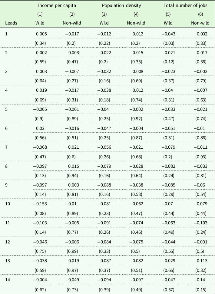
Note: This table summarizes the lead-specific effects of bison reintroduction on income per capita, the total number of jobs, and population density in the post-treatment periods. We focus on six wild bison counties and ten non-wild bison counties with bison herds established between 1980 and 2005 as treated units in the SCM analyses. Column (1), (3), and (5) present the average effects of wild bison herd establishment on local economic health. Column (2), (4), and (6) present the average effects of non-wild bison herd establishment on local economic health. p-values are in parentheses.
Conclusion
In this paper, we explore patterns in the locations of U.S. bison herd reintroduction and estimate the causal effects of those bison reintroduction on local economic health. We estimate the causal effects with two different econometric approaches: a staggered DID with multiple treatment periods and the SCM.
A simple probit analysis shows that wild bison herds are more likely to be established in counties with high income per capita; when geographic features are included, we see that wild bison herds are more commonly located in places with more grasslands, low precipitation, and low temperature. The naive correlation between income and bison herds might lead planners to think that bison reintroduction will increase per capita income in a county. However, none of the causal inference analyses find any statistically significant effects of bison reintroduction on per capita income, employment, or population density. These results are robust to different identifications and treatment samples we apply.
Why is there no effect of bison reintroduction on local economic activity? Many bison herds were established in pre-existing national monuments, state parks, or preserved areas. Some research shows that the protection of public lands itself may have had minimal impact on the local economy (Jakus and Akhundjanov Reference Jakus and Akhundjanov2019); the addition of bison reintroduction may induce too little difference in land use to affect local economies.
The results of this paper may serve to assuage fears of farm, ranch, and local government leaders that bison reintroduction will harm local economies; no such pattern is supported by the evidence. On the other hand, we also do not find compelling evidence that bison herds increase local economic activity, as is sometimes anticipated by those who support reintroduction.
This paper has several important limitations. First, bison reintroduction may have other benefits that are not captured by the analyses in this paper. For example, bison may interact with dung beetles to improve the ecological functioning of grassland habitats and affect bird habitat and carbon sequestration (Barber et al. Reference Barber, Hosler, Whiston and Jones2019). Furthermore, people may place large non-use values on the expanded existence of bison herds in the grasslands of the U.S. that could only be measured with a large-scale stated preference study. Future work would do well to quantify the non-market benefits of bison reintroduction and provide more information to guide ongoing efforts to restore this iconic mammal to the open lands of the U.S.
Second, this paper focuses on bison herds that have been restored and managed for conservation purposes on largely public or non-profit lands. The commercial bison industry has also expanded in the past few decades in the U.S. (Tielkes and Altmann Reference Tielkes and Altmann2021). Some commercial bison ranchers provide (agri)tourism opportunities in addition to meat production, which may mitigate the effects of reintroducing conservation bison herds in the same region. This paper should be interpreted as estimating the impacts of bison restoration for non-profit conservation purposes in a landscape where commercial bison herds have also been expanding. Future research could further explore the potential substitution effects between commercial and non-commercial herds in terms of (agri)tourism demand and amenity values.
Supplementary material
To view supplementary material for this article, please visit https://doi.org/10.1017/age.2022.13
Acknowledgments
We thank Bill Stewart, Carena van Riper, Paul Gobster for comments on earlier versions of this work. We thank Will Wheeler and conference participants at Northeastern Agricultural and Resource Economics Association and Agricultural & Applied Economics Association for discussion and input. We thank two anonymous reviewers for helpful comments on earlier drafts of the manuscript. Any remaining errors are authors’ responsibility.
Funding statement
Data and code that are necessary to replicate findings in the article are available upon request. This research was supported by USDA-NIFA Grant #2016-68006-24836 and USDA-NIFA Multistate Hatch W4133 Grant #ILLU-470-353.
Conflicts of interest
None.


 Open access