


In many regions around the world, scholarly awareness of the archaeological record is lacking (e.g., Stephens et al. Reference Stephens, Fuller, Boivin, Rick, Gauthier, Kay, Marwick, Armstrong, Michael Barton, Denham, Douglass, Driver, Janz, Roberts, Daniel Rogers, Thakar, Altaweel, Johnson, Sampietro Vattuone, Aldenderfer, Archila, Artioli, Bale, Beach, Borrell, Braje, Buckland, Jiménez Cano, Capriles, Castillo, Çilingiroğlu, Cleary, Conolly, Coutros, Alan Covey, Cremaschi, Crowther, Der, di Lernia, Doershuk, Doolittle, Edwards, Erlandson, Evans, Fairbairn, Faulkner, Feinman, Fernandes, Fitzpatrick, Fyfe, Garcea, Goldstein, Goodman, Guedes, Herrmann, Hiscock, Hommel, Ann Horsburgh, Hritz, Ives, Junno, Kahn, Kaufman, Kearns, Kidder, Lanoë, Lawrence, Lee, Levin, Lindskoug, López-Sáez, Macrae, Marchant, Marston, McClure, McCoy, Miller, Morrison, Matuzeviciute, Müller, Nayak, Noerwidi, Peres, Peterson, Proctor, Randall, Renette, Schug, Ryzewski, Saini, Scheinsohn, Schmidt, Sebillaud, Seitsonen, Simpson, Sołtysiak, Speakman, Spengler, Steffen, Storozum, Strickland, Thompson, Thurston, Ulm, Cemre Ustunkaya, Welker, West, Williams, Wright, Wright, Zahir, Zerboni, Beaudoin, Garcia, Powell, Thornton, Kaplan, Gaillard, Goldewijk and Ellis2019). Remote sensing offers not only a unique source for the generation of new archaeological knowledge but also new opportunities to evaluate preexisting data derived through ground-based survey (e.g., Bennett et al. Reference Bennett, Welham, Hill, Ford, Cowley, Opitz, Opitz and Cowley2013; Davis and Douglass Reference Davis and Douglass2020; Lambers et al. Reference Lambers, Verschoof-van der Vaart and Bourgeois2019; McCoy Reference McCoy2017; Opitz and Herrmann Reference Opitz and Herrmann2018; Thompson et al. Reference Thompson, Arnold, Pluckhahn and VanDerwarker2011; also see Ullah Reference Ullah2015). Airborne lidar, in particular, has led to an exponential increase in our ability to identify archaeological deposits (e.g., Chase et al. Reference Chase, Chase, Fisher, Leisz and Weishampel2012; Evans et al. Reference Evans, Fletcher, Pottier, Chevance, Soutif, Tan, Im, Ea, Tin, Kim, Cromarty, De Greef, Hanus, Baty, Kuszinger, Shimoda and Boornazian2013; Guyot et al. Reference Guyot, Hubert-Moy and Lorho2018). Although remote sensing studies typically focus on the identification of novel features (e.g., Davis and Douglass Reference Davis and Douglass2020; Vining Reference Vining2018), there is substantial potential to integrate airborne lidar with existing data derived from ground-based surveys to produce more comprehensive models of settlement patterns (Borie et al. Reference Borie, Parcero-Oubiña, Kwon, Salazar, Flores, Olguín and Andrade2019; Cerrillo-Cuenca and Bueno-Ramírez Reference Cerrillo-Cuenca and Bueno-Ramírez2019). Ground testing, however, remains a crucial step before this information is incorporated into larger analyses (Ainsworth et al. Reference Ainsworth, Oswald, Went, Opitz and Cowley2013; Davis Reference Davis2019; Quintus et al. Reference Quintus, Day and Smith2017).
Here, we demonstrate a means by which remotely sensed information pending ground-testing can be assessed for validity, and by extension, increase archaeological sample sizes without risking the quality of analyses. Ground testing remains crucial, but we argue that pending data can still be utilized, as long as certain evaluations are made prior to their incorporation. Our approach focuses on the application and evaluation of point-process models fitted to ground-truthed and remotely sensed archaeological datasets to evaluate whether they are explained by similar spatial processes. We evaluate the distribution of shell rings, a type of circular midden deposit composed of fresh and/or saltwater shellfish remains, using a combination of legacy and remotely sensed data and spatial modeling.
In the American Southeast, pre-European-contact shell-ring deposits are known to have been primarily occupied during the Late Archaic period (ca. 4800–3200 cal BP; Trinkley Reference Trinkley, Goodyear and Hanson1989). Despite great archaeological interest in shell rings (e.g., Drayton Reference Drayton1802; Cannarozzi and Kowalewski Reference Cannarozzi and Kowalewski2019; Hill et al. Reference Hill, Lattanzi, Sanger and Dussubieux2019; McKinley Reference McKinley1873; Moore Reference Moore1897), our knowledge of these features is largely ad hoc and based on individual studies of deposits (see, for example, Russo Reference Russo2006). Consequently, their presence and distribution across the Southeastern landscape continues to challenge explanations.
Remote sensing offers a means of addressing this deficiency. Davis and colleagues (Davis, Sanger et al. Reference Davis, Lipo and Sanger2019), for example, developed a semiautomatic remote-sensing survey method using object-based image analysis (OBIA) and airborne lidar data to identify artificial mound and ring features systematically. Using this method, the authors used airborne lidar data from Beaufort County, South Carolina (Figure 1), an area that is known for its abundant archaeological record but that has only been intensively surveyed using pedestrian methods over less than 10% of its area (Davis, Sanger et al. Reference Davis, Lipo and Sanger2019). Although the data only offered four bare-ground elevation points for every square meter, these analyses ultimately added over 40 potential shell-ring features of varying sizes to the list of known deposits for the area. Their results suggest the presence of a pre-European-contact landscape in the American Southeast that consists of more numerous shell-ring deposits that are also substantially smaller than those previously identified. Most of these features are located in under-surveyed regions, and the overall results indicate that past discoveries have likely been biased by targeted and patchy investigations. Although we have yet to evaluate all of the findings, subsequent ground surveys support this finding (Figures 2 and 3) and suggest that many more will be confirmed as precontact shell-ring deposits in the future (Davis, Lipo et al. Reference Davis, Sanger and Lipo2019; Davis, Sanger et al. Reference Sanger, Quitmyer, Colaninno, Cannarozzi and Ruhl2019).

FIGURE 1. Map of Beaufort County, South Carolina.

FIGURE 2. Examples of vegetation cover found during ground survey of a new shell-ring site (site ID pending). (a) Digital elevation model (DEM) of ring. The black box represents the location of (b) and (c). (b) Image shows a view of the shell arc, which is difficult to distinguish because of the vegetation. (c) Another view of the shell arc. Photographs by Matthew Sanger.
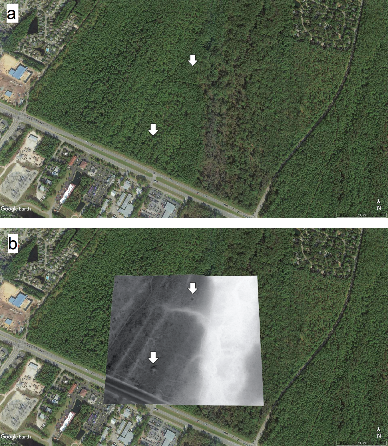
FIGURE 3. Top panel: view of two new archaeological features (site IDs pending) (white arrows) from true-color satellite imagery. Bottom panel: DEM view of the same two archaeological features (white arrows). The ring feature (bottom arrow) is clearly visible from the airborne lidar data, but on the ground (see Figure 2) it is almost impossible to see.
In this article, we use this newly expanded dataset of shell-ring deposits to explore settlement patterns among the Late Archaic populations in Beaufort County, South Carolina. Turning to spatial statistics and point-process modeling, we provide a framework for evaluating ground-truthed and suspected data in terms of evidence related to the identification of past settlement patterns. By comparing distributional patterns of confirmed legacy datasets and remotely identified features, we illustrate how the use of spatially explicit models can aid in the creation of robust archaeological information to inform on spatial questions of site placement.
Specifically, we focus on evaluating hypotheses regarding the factors that best account for the location of shell-ring features on the landscape. We use spatial statistics and point-process modeling to evaluate the degree to which the locations of shell rings are explained by the presence of particular environmental resources (i.e., rivers and water bodies, soil permeability, and elevation), or if additional factors are required. Although our case study focuses on specific feature types, our study provides a framework by which other archaeologists can incorporate remotely sensed and preexisting datasets into larger-scale spatial analyses of archaeological settlement patterns around the world.
SHELL-RING STUDIES IN THE AMERICAN SOUTHEAST
Shell rings are circular midden deposits composed of marine and terrestrial plant and animal remains that generally contain a central plaza devoid of midden material (Russo Reference Russo2006; Sanger Reference Sanger2017; Sanger and Ogden Reference Sanger and Ogden2018). Many researchers account for rings as loci for residential and domestic activities of nucleated communities. (e.g., Crusoe and DePratter Reference Crusoe and DePratter1976; Thompson and Andrus Reference Thompson and Andrus2011; Trinkley Reference Trinkley, Dickens and Trawick Ward1985). Evidence from the excavations of ring deposits generally supports the notion that these locations were occupied year-round, given that the variety of faunal and botanical species present in these deposits indicates use during all four seasons (Calmes Reference Calmes1968; Sanger et al. Reference Sanger, Quitmyer, Colaninno, Cannarozzi and Ruhl2019; Thompson and Andrus Reference Thompson and Andrus2011; Trinkley Reference Trinkley1980, Reference Trinkley, Dickens and Trawick Ward1985). For example, the presence of some fish species suggests year-round activity (Thompson and Andrus Reference Thompson and Andrus2011). In other cases, the deposits include shellfish that would have been harvested for only a fraction of the year, suggesting that occupation was seasonal (Sanger et al. Reference Sanger, Quitmyer, Colaninno, Cannarozzi and Ruhl2019). In some instances, these patterns change over time: whereas early residents may have been present year- round, later occupants were only present in one or two seasons (Thompson and Andrus Reference Thompson and Andrus2011). Some researchers suggest that rings were also locations for episodic events (Sanger et al. Reference Sanger, Hill, Lattanzi, Padgett, Larsen, Culleton, Kennett, Dussubieux, Napolitano, Lacombe and Thomas2018, Reference Sanger, Quitmyer, Colaninno, Cannarozzi and Ruhl2019; Trinkley Reference Trinkley, Dickens and Trawick Ward1985). For example, the possibility that Native Americans used some shell rings as gathering places, perhaps for ceremonial activities, has been strengthened by the discovery of a multiple-person cremation in the center of one ring (Sanger et al. Reference Sanger, Hill, Lattanzi, Padgett, Larsen, Culleton, Kennett, Dussubieux, Napolitano, Lacombe and Thomas2018).
Not all researchers agree that shell rings are solely the consequence of residential and ceremonial activities. Marquardt (Reference Marquardt2010), for example, argues that the morphology of ring features is due to precontact populations creating these deposits as basins for holding drinking water. According to this hypothesis, communities created shell rings during periods of low water availability, and these circular deposits held water acquired through rainfall, from excavated wells, or by capturing outflow from nearby streams (Middaugh Reference Middaugh2013).
The discovery of over 40 additional ring sites in Beaufort County, South Carolina, has expanded the available sample size of these features and offers an opportunity to statistically explore patterns among their morphology and locations. Specifically, we have sufficient examples of shell rings to examine how deposit locations and shapes are related to environmental resources and constraints. Assuming that rings serve as localized sites of community investment over substantial lengths of time, and that these deposits represent activities that are central to the communities of which they are part, we can assess the degree to which their occurrence is systematically connected to aspects of the environment—such as distance from water sources, topography, and soil productivity—and the degree to which other factors have to be included.
To accomplish this task, we develop a series of spatial point-process models that examine the relationship between shell-ring attributes, deposit locations, and environmental variables. Given the composition of these rings of shell remains, we assume that locations where shellfish are abundant strongly contribute to the determination of deposit location. Consequently, we assess the degree to which the distance to water bodies (i.e., rivers, oceans, etc.) statistically accounts for the positions that shell rings take on the landscape. If shell-ring location is tied primarily to residential activity, we would expect to see deposits preferentially appearing on particular portions of the landscape. Specifically, given the degree of regular flooding that takes place on the coastal plains, year-round habitation would have required utilizing locations that remained nominally dry. Consequently, we expect that dry land factored into the locations of shell rings, particularly high-elevation areas with well-drained soils and at relatively large distances from water sources. If, however, shell rings served primarily as structures for water retention, as argued by Marquardt (Reference Marquardt2010) and Middaugh (Reference Middaugh2013), we expect that they would preferentially appear in lower-lying areas with poorly drained soils and in relatively close proximity to water sources.
METHODS
In our analyses, we use a sample of 52 rings that consist of 42 highly likely ring deposits from the Davis, Sanger, and Lipo study (Reference Davis, Sanger and Lipo2019; Table 1; Figure 4; Supplemental Table 1) as well as 10 confirmed rings from that study and previous research (see Russo Reference Russo2006). We assess morphological diversity of the “likely” deposits identified in airborne lidar using Friedman's independence tests to compare with pre-identified rings. Then, we analyze the spatial patterns of these rings and develop a series of point-process models to assess their relationship with environmental variables. Because the data contain confirmed (i.e., ground-truthed) rings and features that are identified as having a high likelihood of being shell rings by lidar and OBIA, we run the same point-pattern analyses on (1) the confirmed ring deposits (n = 10) located within the study area (Beaufort County), (2) the potential rings identified in airborne lidar data (n = 42), and (3) the combined data (n = 52). By comparing confirmed rings to suspected rings, our analysis can detect any strong divergence between the pattern of confirmed shell rings and the combined dataset. If the patterns found in confirmed rings are similar to the results found in “likely” rings, we can include these features into the point-pattern analysis to assess environmental relationships with a larger sample size.
TABLE 1. Comparison between Russo's Calculations of Average Shell-Ring Diameters and Potential Rings Identified by Remote-Sensing Survey.


FIGURE 4. Map of ring locations used for comparison against Russo’s (Reference Russo2006) dataset. Features are labeled by FID, corresponding to Supplemental Table 1.
To assess whether shell-ring features in our study area exhibit clustered or dispersed patterns, we calculate the nearest neighbor distances among shell rings and their pair correlation function (see Baddeley et al. Reference Baddeley, Rubak and Turner2015:225; Stoyan and Stoyan Reference Stoyan and Stoyan1994). We use the pair correlation function g(r) to assess whether a point pattern is significantly more clustered or dispersed than expected for a random pattern. We then compare the empirical pair correlation function for shell rings against 999 simulated realizations of complete spatial randomness (CSR, equivalent to p = 0.002).
To examine the relation between shell rings (confirmed [n = 10], “likely” [n = 42], and the combined sample [n = 52]), we use three different environmental variables: distances to water sources (i.e., rivers, streams, etc.), elevation, and soil drainage properties. We use locations for water derived from United States Geological Survey (USGS) land-use maps (http://www.gis.sc.gov/) and elevation values from the National Oceanic and Atmospheric Administration's (NOAA) digital elevation models (DEMs; https://coast.noaa.gov/dataviewer/). For spatial tests, however, we modify the original DEM to fill all holes using the elevation “void fill” function in ArcGIS (version 10.7; ESRI 2018), which uses inverse distance weighting (IDW) interpolation to fill missing data values in DEMs. We then resample the data to downscale the DEM to 3 m spatial resolution.
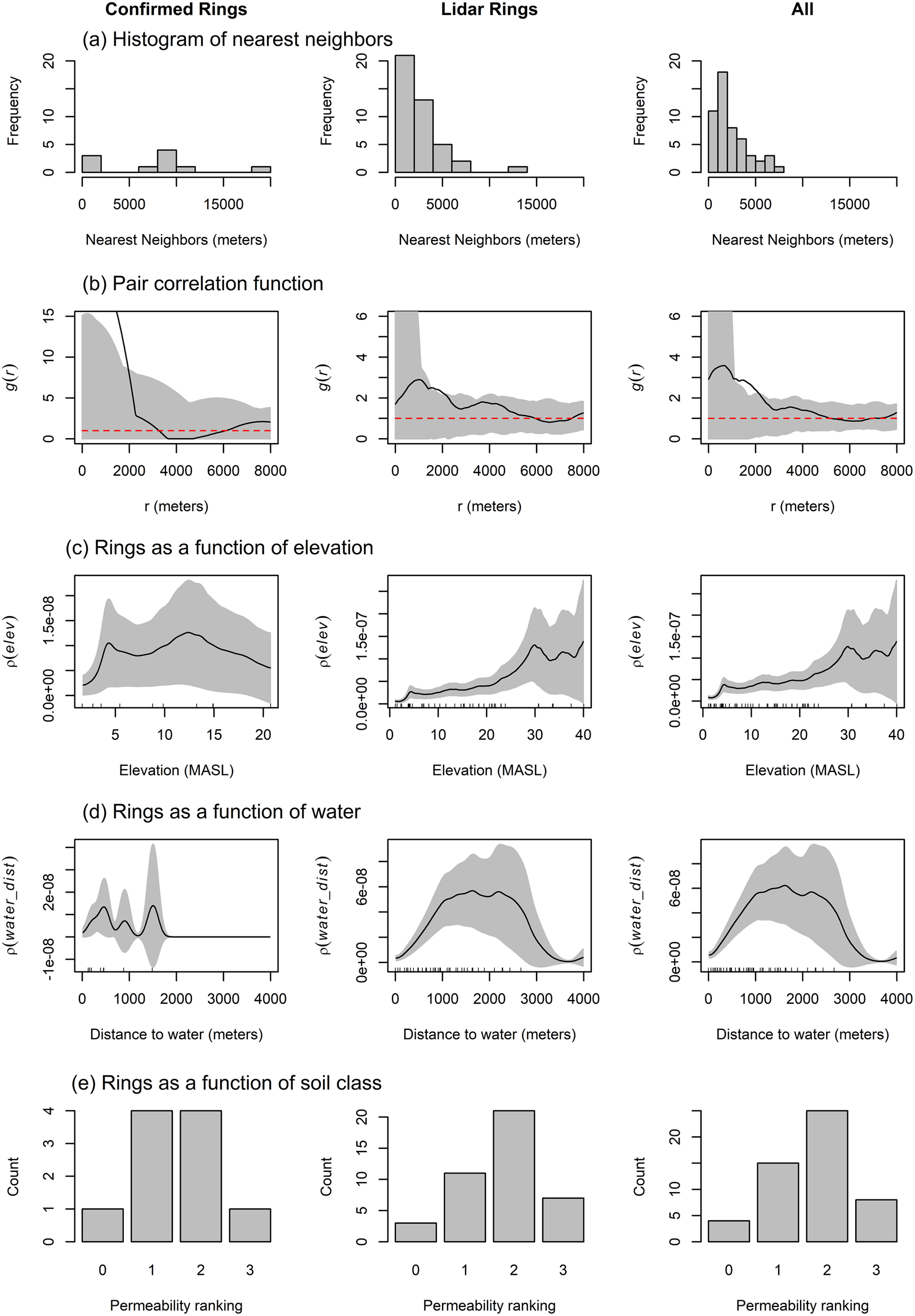
Finally, we use soil data from the South Carolina Department of Natural Resources GIS Clearinghouse repository (http://www.dnr.sc.gov/pls/gisdata/) to assess the drainage characteristics following the United States Department of Agriculture (USDA) Official Soil Series Descriptions (accessed through https://soilseries.sc.egov.usda.gov/osdname.aspx). Once recorded, we convert the soil permeability rankings into a simplified numerical index that ranges from 1 (slow) to 3 (rapid) permeability.Footnote 1 The relations among the intensity of shell rings and these three variables are shown in Figure 5. The upper-left plot in Figure 5 shows the kernel density estimate for shell rings. In this kernel density estimate, we select the smoothing bandwidth by likelihood cross-validation (for more details, see Baddeley et al. Reference Baddeley, Rubak and Turner2015:171, 189).

FIGURE 5. Relations among the intensity of shell rings (n = 52) (top left) and elevation in meters (top right), distance to water in meters (bottom left), and soil permeability (bottom right). Confirmed rings are represented by red squares. Highly likely rings are represented by blue circles.
To assess the importance of the variables selected above, we create a series of point-process models to assess the degree to which each variable accounts for spatial patterns in the empirical record, following the methods recently presented in DiNapoli and colleagues (Reference DiNapoli, Lipo, Brosnan, Hunt, Hixon, Morrison and Becker2019) and Eve and Crema (Reference Eve and Crema2014). We begin by building a null model that assumes the underlying process for the observed pattern is complete spatial randomness (CSR, a homogeneous Poisson process). We then build a series of additional, inhomogeneous Poisson models, which model the intensity of shell rings as a log-linear function of the following variables: distance from water sources, soil permeability, and elevation. We also build models that account for potential clustering or dispersion between points in addition to the effects of spatial covariates. For these latter models, we model interpoint interaction using a Gibbs area-interaction process, which is a flexible point-process model that allows for both clustering or dispersion at varying scales (Baddeley and Van Lieshout Reference Baddeley and Marie-Colette1995; Baddeley et al. Reference Baddeley, Rubak and Turner2015).
To evaluate the fit between each of these models and the empirical spatial pattern of shell rings, we employ a series of model-validation procedures based on simulation envelopes (Baddeley et al. Reference Baddeley, Rubak and Møller2011, Reference Baddeley, Diggle, Hardegen, Lawrence, Milne and Nair2014) and multimodel selection based on the relative differences between models in Akaike Information Criterion (AIC; Akaike Reference Akaike1974) and Bayesian Information Criterion (BIC; Schwarz Reference Schwarz1978) scores and their associated weights to choose the best fitting model. Model selection tools such as AIC and BIC allow for the formal comparison of different statistical models applied to the same dataset by evaluating the trade-off between how well a given model fits the data (e.g., likelihood) and its complexity (Burnham and Anderson Reference Burnham and Anderson2002). The best models are those that account for the most variability in the data in the simplest way. The smallest change in information criterion score (ΔAICc and ΔBIC) and highest weight values (wi) indicate the best-fitting model. Because our sample size is small relative to the number of maximum parameters in the models evaluated, we use a second-order AIC for smaller sample sizes, AICc (Burnham and Anderson Reference Burnham and Anderson2002).
We conduct our point-process analyses in R (version 3.6.1; R Core Team 2019) using the spatstat (Baddeley et al. Reference Baddeley, Rubak and Turner2015) and MuMIn (Barton Reference Barton2019) packages. We also used the maptools (Bivand and Lewin-Koh Reference Bivand and Lewin-Koh2019), raster (Hijmans Reference Hijmans2019), rgdal (Bivand et al. Reference Bivand, Keitt and Rowlingson2019), rgeos (Bivand and Rundel Reference Bivand and Rundel2019), sp (Bivand et al. Reference Bivand, Pebesma and Gomez-Rubio2013; Pebesma and Bivand Reference Pebesma and Bivand2005), here (Müller Reference Müller2017), and readxl (Wickham and Bryan Reference Wickham and Bryan2018) packages. All data and R code necessary to reproduce these analyses are available in the supplemental files.
RESULTS
The locations of the rings identified by Davis and colleagues (Davis, Sanger et al. Reference Davis, Lipo and Sanger2019) all fall within forests, marshland, and swamps (Table 2). As noted in the previous study (Davis, Sanger et al. Reference Davis, Lipo and Sanger2019), the results in Table 2 suggest that prior surveying in certain types of land cover (specifically swamps and dense forests) has been limited in success, resulting in dozens of unidentified ring features throughout the study area.
TABLE 2. Geographic Locations of Identified Ring Features.

a Land types classified by USGS.
b Davis, Lipo et al. Reference Davis, Sanger and Lipo2019; Davis, Sanger et al. Reference Sanger, Quitmyer, Colaninno, Cannarozzi and Ruhl2019.
c Land percentages are based on all areas where rings were found.
d Russo Reference Russo2006.
The sizes of the identified shell rings show that the features found through remote sensing are smaller than those previously identified from pedestrian surveys (Friedman χ2 = 6, df = 2, p < 0.05; Supplemental Text 1). The smaller size and volume of these shell rings points to the fact that shell rings were not limited to just large aggregates of populations—they likely served groups of varying sizes.
When examining the spatial distribution of confirmed shell rings in Beaufort County (n = 10), exploratory analysis shows that they occur on locations that have relatively high elevations, that are significantly large distances from water sources, and that are within moderate-to-high permeability soil classes (Figure 6 ). The pair correlation function for confirmed rings shows that the features are clustered at distances around 2,000 m (Figure 6). The point-process model results for confirmed rings suggests that the spatial pattern of shell rings is best accounted for by an area-interaction cluster model (Baddeley et al. Reference Baddeley, Rubak and Turner2015; Supplemental Text 2). The model selection for the confirmed rings data suggests that a simple cluster model fits better than a model with clustering and an elevation covariate, but that models with an elevation covariate are highly ranked. In other words, the model selection suggests that the confirmed ring features are distributed as a series of randomly placed clusters. The seemingly random distribution of confirmed rings is likely the consequence of the opportunistic, rather than systematic, survey strategy that identified many of these features.

FIGURE 6. Relationship among shell-ring features (confirmed, n = 10; “likely,” n = 42; total sample, n = 52). First row (a) shows histogram of nearest-neighbor distances. Second row (b) shows pair-correlation (g(r)) function. The black line shows the observed value of g(r) for the pattern of shell rings, the red dashed line is the theoretical value of g(r) under CSR, and the gray shading is the upper and lower bounds of the pointwise simulation envelopes of g(r) based on 999 simulations of CSR (p = 0.002). Remaining rows show the relationship between shell rings and elevation (c), distance to water (d), and soil permeability ranking (e). Rows 3 and 4, respectively, show a smoothed estimate of the intensity of shell rings as a function of elevation and water (with 95% confidence bands). Row 5 (e) shows the counts of shell rings by soil permeability class (0 = no information available, 1 = low permeability, 2 = medium permeability, 3 = fast permeability).
Analysis of the data set of “highly likely” rings (n = 42) identified using OBIA and aerial lidar data resulted in somewhat similar results for the exploratory analyses, which indicate that rings are clustered and occur in high elevations, at large distances from water sources, and within higher permeability soils (Figure 6). Point-process modeling and multimodel selection indicate that an area-interaction cluster model with an elevation covariate fits best, meaning that the OBIA-identified rings occur as a series of clusters in relatively high-elevation areas (Supplemental Text 2). As the results for the confirmed and OBIA-identified rings show similar first- and second-order spatial patterns, we proceed to combine both datasets to assess shell-ring distribution with a more robust, systematic dataset.
Figure 6 shows patterns among all shell-ring features within the study area. The distribution of nearest neighbor distances suggests that most shell rings lie about 2,000 m apart, a distance that is supported by the pair-correlation function that shows significant clustering at distances between approximately 1,500 and 2,000 m. The relationship between the spatial intensity of shell rings and elevation, distance to water, and soil permeability ranking are shown in Figure 6. These results show that the density of shell rings increases with elevation, that it initially increases with distance from water up to distances of about 1,000 m and then plateaus, and that shell rings appear most often on soils with medium permeability (class 2). Together, these exploratory results suggest that shell rings within our study area tend to be clustered at relatively high elevations on moderately drained soils and at relatively large distances from water sources, and therefore are in agreement with the confirmed sample of rings.
The results of the multimodel selection are shown in Table 3. Comparison of a homogeneous Poisson process model (i.e., CSR) and inhomogeneous Poisson models with different combinations of our three environmental variables suggest that elevation is the best predictor of shell-ring intensity. The elevation model (Model 2) has ΔAICc = 0 and wi = 0.635 and a ΔBIC = 0 and wi = 0.856. Although Model 2 offers the best fit given these inhomogeneous Poisson models, overall, the empirical pattern may still deviate from model expectations, in particular due to second-order interaction properties of the point pattern (e.g., clustering). As a model validation procedure, we compared the empirical distribution of shell rings to expectations from the model using 99 Monte Carlo simulations of the residual K- and G-functions. Figure 7 shows the model validation results, indicating that the empirical pattern of shell rings is more clustered than is accounted for by Model 2.
TABLE 3. Multimodel Comparison for Inhomogeneous Poisson Models.


FIGURE 7. Results of model validation for possible interaction components in Model 2 using Monte Carlo simulations of the residual K- (left) and G-functions (right). The black line shows the empirical function for shell rings, the dashed red lines are the theoretical expectation under model assumptions, and the gray envelope is based on 99 simulations from the model. Both tests indicate that the empirical pattern of shell rings is more clustered than is accounted for by Model 2.
Given this deviation between Model 2 and the data, we constructed two additional models to account for clustering among shell rings using a Gibbs area-interaction process. The first (Model 8) simply models the pattern of shell rings as a function of interpoint clustering with no environmental variables. This serves to test the hypothesis that the point pattern is simply explained by interpoint clustering and not elevation. The second (Model 9) incorporates both a second-order interaction component and the elevation covariate. The value of the irregular clustering parameter (r) was set to 2,000 m for both models based on the nearest neighbor distribution and pair-correlation function for shell rings (Figure 6). Comparison of these two cluster models with the best-fitting inhomogeneous Poisson model (Model 2) suggests that Model 9, incorporating both an area-interaction component and elevation, fits best with ΔAICc = 0 and wi = 0.97 and ΔBIC = 0 and wi = 0.93 (see Table 4).
TABLE 4. Multimodel Comparison for Best-Fitting Inhomogeneous Poisson Model 2 and Gibbs Area-Interaction Models 8 and 9.

Table 5 shows the covariate estimates for the best-fitting cluster Model 9, and Figure 8 shows model validation plots for Model 9. The residual K- and G-functions assess the fit between the interaction (i.e., clustering) component of model, and the lurking-variable and partial-residual plots assess any deviations between the empirical intensity of shell rings and their fitted intensity as a function of elevation (Baddeley et al. Reference Baddeley, Chang, Song and Turner2013, Reference Baddeley, Rubak and Turner2015:419–425). The lurking-variable plot shows the relationship between the residuals and elevation, and the partial-residual plot shows the relationship between the estimated intensity as a function of elevation and a smoothed estimate of its empirical effect. Overall, these residual diagnostics suggest that there is a good fit between both the first- and second-order components of the model and the empirical point pattern, but that the model is underestimating the intensity at elevation values less than or equal to 5 m.
TABLE 5. Results of the Best-Fitting Model 9 Incorporating an Area-Interaction Component and Elevation Covariate.


FIGURE 8. Model diagnostics for best-fitting Model 9 incorporating an Area Interaction component and elevation covariate. Residual K- (top left) and G-functions (top right) show fit between the empirical second-order interaction component and the model. Lurking-variable (bottom left) and partial-residual (bottom right) show the relationship between the empirical intensity of shell rings and their fitted intensity as a function of elevation (gray shading represents 95% confidence intervals). The blue line in the partial residual plot is the fitted intensity and the black is the empirical intensity as a function of elevation.
The analysis presented above includes confirmed (i.e., ground-truthed) features and features that OBIA identified as having a high likelihood of being shell rings. Although there is a possibility that some of the rings identified by OBIA are false positives, we ran the same analysis presented above on only confirmed rings (n = 10) and obtained similar results (Supplemental Text 2). This result provides support that the “highly likely” ring features are indeed precontact deposits although they have yet to be ground tested. Because of the small sample size and biased nature of the confirmed data, slight differences between the results of the confirmed dataset and the unconfirmed data are likely the result of the unrepresentative nature of the surveys that generated confirmed ring data.
DISCUSSION
The incorporation of lidar-derived shell-ring features with preexisting datasets allows for a robust analysis of otherwise scarce features within the landscapes of the American Southeast. Because confirmed rings were previously identified through opportunistic means (see Russo Reference Russo2006), earlier evaluation of the distribution of these sites was limited to a small and likely biased dataset. The identification of dozens more shell rings, however, evidences a more prevalent ring-building tradition. Recent research along the Georgia Coast (Turck and Thompson Reference Turck and Thompson2016) suggests that shell-bearing sites, particularly shell rings, were the primary means by which people occupied the coastline prior to approximately 3800 cal BP. Our identification of dozens of additional potential rings strengthens this conclusion and demonstrates a more widely distributed population in the region that extends beyond the presence of only a few centralized locales.
When comparing the set of shell rings identified by OBIA with preexisting data, identical spatial tests yielded comparable results, thereby increasing the validity of the conclusion that the features identified using airborne lidar and OBIA are precontact anthropogenic deposits. Although the confirmed data are probably not representative of the full distribution and variation of ring features, the similarity between the results of our analyses on confirmed and remotely identified rings increases the likelihood that the patterns observed among the remotely sensed features are valid. Consequently, these data provide a solid baseline by which to evaluate spatial patterns in shell rings within Beaufort County, South Carolina. We stress that the interpretations we present here are best used as model-based working hypotheses, and formal ground testing is still required for confirmation.
In addition to demonstrating how airborne lidar datasets can be incorporated into larger studies of site distribution, our study assists in developing a greater understanding of the factors involved in shell-ring placement in the American Southeast. The results of our point-process models and model selection suggest that elevation—rather than the distance to marine sources—provides the best prediction for where shell rings occur. This finding fits results from other studies in the Southeast that suggest elevation was actively preferred by Native Americans in their settlements (e.g., Guccione et al. Reference Guccione, Lafferty and Cummings1988; Mehta and Chamberlain Reference Mehta and Chamberlain2019; Smith Reference Smith and Smith1978). Although our analyses demonstrate that people were building rings farther from water sources than previously assumed, it does not mean marine resources were unimportant. Instead, it suggests that in a context where water is ubiquitous, occupations can be placed at a greater distance to water without compromising access to these resources. When evaluating ring distribution with respect to water connectivity, most rings were located at distances of 1–3 km from waterways. Many were equidistant from waterways that connected to other rings. The presence of water, however, is not a strong predictor of shell-ring location compared to other variables.
Even though elevation is the strongest predictor of ring placement, it does not completely account for the pattern of shell rings. Our modeling shows that shell rings are highly clustered even when one accounts for their tendency to be in high-elevation areas. This result is significant because it indicates that some process is leading to second-order interaction (clustering) among rings (discussed below). In addition, the model diagnostic results shown in Figure 8 suggest that the first-order intensity of shell rings is not completely accounted for by elevation, with the lurking variable plot showing deviations at elevations around 5 m. This finding suggests that there is probably an extant variable (or set of variables) in lower-elevation areas that we have not accounted for that is influencing the intensity of shell rings. Future work should explore other variables that may play a role in ring placement.
It is also worth mentioning the possibility that the importance of elevation could be related to preservation or visibility issues. Higher elevation, for example, could result in better protection for rings from erosion. It is also possible, however, that sites closer to sea level (at lower elevations) would not necessarily erode away at higher rates but would instead be infilled by soil deposition. As such, shell rings in lower elevations would likely become less visible over time as they were inundated and filled with sediment.
Clustering among rings is probably the result of social and/or economic processes, in addition to environmental context. Shell and shell-bearing deposits have been associated with spiritual significance, political hierarchy, and social groupings (Anderson Reference Anderson, Gibson and Carr2004; Claassen Reference Claassen, Andrzej and Roberto2008; Deter-Wolf and Peres Reference Deter-Wolf, Peres and Peres2014; Russo Reference Russo, Gibson and Carr2004), and prior work has demonstrated that marine resources are not always a determining factor for the placement of shell deposits in the U.S. Southeast (Claassen Reference Claassen2010). Furthermore, with the recent discovery of human burials at shell-ring sites (Sanger et al. Reference Sanger, Hill, Lattanzi, Padgett, Larsen, Culleton, Kennett, Dussubieux, Napolitano, Lacombe and Thomas2018), rings likely carried a “claim” to particular locations (Deter-Wolf and Peres Reference Deter-Wolf, Peres and Peres2014; Gamble Reference Gamble2017; Rodning Reference Rodning2009). Future work using measures of morphological variability among rings will be needed to test hypotheses regarding sociopolitical systems and adaptive evolutionary strategies. Rings clearly vary in size, as indicated by the new ring data in comparison to preexisting information.
As recent studies have demonstrated (Hill et al. Reference Hill, Lattanzi, Sanger and Dussubieux2019; Sanger et al. Reference Sanger, Hill, Lattanzi, Padgett, Larsen, Culleton, Kennett, Dussubieux, Napolitano, Lacombe and Thomas2018), shell rings were also involved in long-distance trade networks. Exchange networks may have facilitated displays of exotic goods used to signal individual or group-level status (Sanger et al. Reference Sanger, Hill, Lattanzi, Padgett, Larsen, Culleton, Kennett, Dussubieux, Napolitano, Lacombe and Thomas2018). In this case, the clustering of rings could be the result of social signaling practices (sensu Bliege Bird and Smith Reference Bliege Bird and Smith2005; Roscoe Reference Roscoe2009). Mounded architecture has also been explained as a bet-hedging strategy (Peacock and Rafferty Reference Peacock, Rafferty, Fontijn, Louwen, Vaart and Wentink2013), whereby mounds were constructed as a way for groups to buffer themselves against environmental fluctuations. Although waterways do not seem to be a strong predictor of ring distribution, it is possible that terrestrial networks between rings could have influenced settlement decisions. Further work is needed to test these hypotheses.
One additional possibility that is beyond our current ability to evaluate, but that would be useful in future research, is that ring distributions are related to temporal differences. It is quite likely that these ring features were built over the course of hundreds, if not thousands, of years, and they may not represent contemporary or continuous occupations. As such, the distributional pattern observed in the record today may be in part due to temporal overlap, with communities repeatedly choosing to locate in the same locations over time. Our analyses, however, indicate that the presence of rings is a strong predictor of other rings. The evidence presented here suggests that people deposited material that forms rings in the same locations, rather than move to new areas. This pattern is likely due in part to environmental context (as our models indicate), but almost certainly included aspects of social interaction among groups. Although sample size might be a factor, this result is supported by the fact that there are many places in the landscape that contain these environmental characteristics, yet no rings are found (see Figure 5).
With the presence of rings that are considerably smaller than currently documented features, hypotheses regarding ring uses are in need of reevaluation. For example, the monumental construction hypothesis (Russo Reference Russo, Gibson and Carr2004; Russo and Heide Reference Russo and Heide2003; Saunders Reference Saunders, Saunders and Hays2004) may not be broadly applicable. Instead, they may only be useful in interpreting much larger shell rings. Likewise, interpreting shell rings as circular dams (Marquardt Reference Marquardt2010; Middaugh Reference Middaugh2013) is not consistent with the overall distribution of shell rings based on the current analyses. Additional studies at these smaller rings are needed to better understand their formational histories and address these hypotheses. Nonetheless, their presence shows that shell-ring morphology is probably far more diverse than previously assumed, meaning that the activities associated with shell-ring deposits were likewise diverse.
A final implication of this research pertains to the location of shell rings with respect to sea-level changes. Archaeologists have long assumed that coastal people were building rings throughout the Late Archaic as sea levels were rising (Russo Reference Russo2006). Consequently, we often assume that many rings are now covered by water and that we have lost that portion of the archaeological record. There is some limited evidence to support this hypothesis—several rings are currently located at the edge of waterbodies or are periodically flooded at high tide (Russo Reference Russo2006). Given that sea levels were approximately 4 m lower than present levels during the Archaic (DePratter and Howard Reference DePratter and Howard1981; Gayes et al. Reference Gayes, Scott, Collins, Nelson, Fletcher and Wehmiller1992), it is possible that the earliest rings are simply eroded or buried under silt deposits below current sea levels. Our findings, however, suggest that these rings found on the water's edge are a rarity and that most rings are located at higher elevations. The confirmed Archaic rings located within Beaufort County, South Carolina, for example, have an average elevation of over 10 m, placing them well above both current and Archaic-period sea levels. Therefore, ring formation may have begun while sea levels were rising, but they may have actively increased after sea levels stabilized near modern levels. Of course, ground confirmation and absolute age determination for construction events are needed to assess this hypothesis. If correct, it is likely that this information would reshape our understanding of shell-ring activity and the people who built them, as well as improve the ability of researchers to locate more of these deposits throughout the American Southeast.
It is also important to note that the pattern of shell-ring placement may be regionally distinct, and rings constructed further south may display different patterns with respect to environmental context. Additionally, the identification of submerged features is stymied by poor preservation, visibility issues, and difficult survey conditions that often require expensive equipment and time-consuming processes (Missiaen et al. Reference Missiaen, Sakellariou, Flemming, Bailey, Harff and Sakellariou2017). As such, it is possible that many submerged rings exist, but they are yet to be identified by archaeologists.
CONCLUSION
With the growth of remote sensing as a tool for generating information about the archaeological record, we are now able to iteratively evaluate the degree to which earlier ground-based approaches generated representative samples of settlement pattern data and the efficacy of remotely identified features (Bennett et al. Reference Bennett, Welham, Hill, Ford, Cowley, Opitz, Opitz and Cowley2013; Opitz and Herrmann Reference Opitz and Herrmann2018; Vining Reference Vining2018). Such efforts are crucial for larger analyses, as the integration of remotely sensed observations with legacy datasets yields significantly greater sample sizes that offer more complete data on the processes responsible for the distribution and patterning of past settlements (e.g., Cerrillo-Cuenca and Bueno-Ramírez Reference Cerrillo-Cuenca and Bueno-Ramírez2019; Ullah Reference Ullah2015). Here, we demonstrate one way these goals might be achieved through point-process modeling of data derived from semiautomated analysis of airborne lidar and legacy datasets.
Our framework for evaluating ground-truthed and remotely sensed data in terms of their distributional patterns demonstrates how the use of spatially explicit models can allow for the potential integration of these data and robust investigations of processes leading to site distributions. For areas without broad archaeological knowledge, this approach can aid greatly in the generation of larger datasets that are necessary to evaluate long-standing questions regarding human use of past landscapes. Future landscape archaeologists may find that similar types of model-based analyses are useful means for investigating the robustness of our samples, the quality of our analyses, and the validity of our results.
Supplemental Material
For supplemental material accompanying this article, visit https://doi.org/10.1017/aap.2020.18.
Supplemental Table 1. List of features used to compare to Russo's (Reference Russo2006) compilation of known rings.
Supplemental Text 1. R code for performing statistical tests on ring data presented in the manuscript.
Supplemental Text 2. Reproducible spatial analysis for shell-ring features in Beaufort County, South Carolina.
Acknowledgments
The authors would like to thank Timothy DeSmet and the Binghamton University Remote Sensing and Geophysics Laboratory for contributing technical support and equipment that started this project. This research was supported by the National Geographic Society (award number HJ-107R-17) and Binghamton University. D.S.D. was supported by the National Aeronautics and Space Administration (Grant No. NNX15AK06H) issued through the Pennsylvania Space Grant Consortium. The authors wish to thank the anonymous reviewers for their constructive comments.
Data Availability Statement
All associated datasets and R code are available from Penn State's ScholarSphere repository at https://doi.org/10.26207/7erq-3662.


 Open access