


1 Introduction
This survey focuses on sequential data assimilation techniques for state and parameter estimation in the context of discrete- and continuous-time stochastic diffusion processes. See Figure 1.1. The field itself is well established (Evensen Reference Evensen2006, Särkkä Reference Särkkä2013, Law, Stuart and Zygalakis Reference Law, Stuart and Zygalakis2015, Reich and Cotter Reference Reich and Cotter2015, Asch, Bocquet and Nodet Reference Asch, Bocquet and Nodet2017), but is also undergoing continuous development due to new challenges arising from emerging application areas such as medicine, traffic control, biology, cognitive sciences and geosciences.
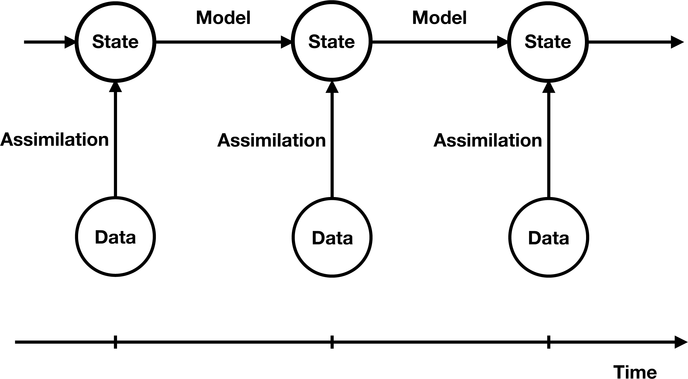
Figure 1.1. Schematic illustration of sequential data assimilation, where model states are propagated forward in time under a given model dynamics and adjusted whenever data become available at discrete instances in time. In this paper, we look at a single transition from a given model state conditioned on all the previous and current data to the next instance in time, and its adjustment under the assimilation of the new data then becoming available.
Data assimilation is typically formulated within a Bayesian framework in order to combine partial and noisy observations with model predictions and their uncertainties with the goal of adjusting model states and model parameters in an optimal manner. In the case of linear systems and Gaussian distributions, this task leads to the celebrated Kalman filter (Särkkä Reference Särkkä2013) which even today forms the basis of a number of popular data assimilation schemes and which has given rise to the widely used ensemble Kalman filter (Evensen Reference Evensen2006). Contrary to standard sequential Monte Carlo methods (Doucet, de Freitas and Gordon Reference Doucet, de Freitas and Gordon2001, Bain and Crisan Reference Bain and Crisan2008), the ensemble Kalman filter does not provide a consistent approximation to the sequential filtering problem, while being applicable to very high-dimensional problems. This and other advances have widened the scope of sequential data assimilation and have led to an avalanche of new methods in recent years.
In this review we will focus on probabilistic methods (in contrast to data assimilation techniques based on optimization, such as 3DVar and 4DVar (Evensen Reference Evensen2006, Law et al.
Reference Law, Stuart and Zygalakis2015)) in the form of sequential particle methods. The essential challenge of sequential particle methods is to convert a sample of
 $M$
particles from a filtering distribution at time
$M$
particles from a filtering distribution at time
 $t_{k}$
into
$t_{k}$
into
 $M$
samples from the filtering distribution at time
$M$
samples from the filtering distribution at time
 $t_{k+1}$
without having access to the full filtering distributions. It will also often be the case in practical applications that the sample size will be small to moderate in comparison to the number of variables we need to estimate.
$t_{k+1}$
without having access to the full filtering distributions. It will also often be the case in practical applications that the sample size will be small to moderate in comparison to the number of variables we need to estimate.
Sequential particle methods can be viewed as a special instance of interacting particle systems (del Moral Reference del Moral2004). We will view such interacting particle systems in this review from the perspective of approximating a certain boundary value problem in the space of probability measures, where the boundary conditions are provided by the underlying stochastic process, the data and Bayes’ theorem. This point of view leads naturally to optimal transportation (Villani Reference Villani2003, Reich and Cotter Reference Reich and Cotter2015) and, more importantly for this review, to Schrödinger’s problem (Föllmer and Gantert Reference Föllmer and Gantert1997, Leonard Reference Leonard2014, Chen, Georgiou and Pavon Reference Chen, Georgiou and Pavon2014), as formulated first by Erwin Schrödinger in the form of a boundary value problem for Brownian motion (Schrödinger Reference Schrödinger1931).
This paper has been written with the intention of presenting a unifying framework for sequential data assimilation using coupling of measure arguments provided through optimal transportation and Schrödinger’s problem. We will also summarize novel algorithmic developments that were inspired by this perspective. Both discrete- and continuous-time processes and data sets will be covered. While the primary focus is on state estimation, the presented material can be extended to combined state and parameter estimation. See Remark 2.2 below.
Remark 1.1. We will primary refer to the methods considered in the survey as particle or ensemble methods instead of the widely used notion of sequential Monte Carlo methods. We will also use the notions of particles, samples and ensemble members synonymously. Since the ensemble size,
 $M$
, is generally assumed to be small to moderate relative to the number of variables of interest, we will focus on robust but generally biased particle methods.
$M$
, is generally assumed to be small to moderate relative to the number of variables of interest, we will focus on robust but generally biased particle methods.
1.1 Overall organization of the paper
This survey consists of four main parts. We start Section 2 by recalling key mathematical concepts of sequential data assimilation when the data become available at discrete instances in time. Here the underlying dynamic models can be either continuous (i.e. generated by a stochastic differential equation) or discrete-in-time. Our initial review of the problem will lead to the identification of three different scenarios of performing sequential data assimilation, which we denote by (A), (B) and (C). While the first two scenarios are linked to the classical importance resampling and optimal proposal densities for particle filtering (Doucet et al. Reference Doucet, de Freitas and Gordon2001), scenario (C) builds upon an intrinsic connection to a certain boundary value problem in the space of joint probability measures first considered by Erwin Schrödinger (Reference Schrödinger1931).
After this initial review, the remaining parts of Section 2 provide more mathematical details on prediction in Section 2.1, filtering and smoothing in Section 2.2, and the Schrödinger approach to sequential data assimilation in Section 2.3. The modification of a given Markov transition kernel via a twisting function will arise as a crucial mathematical construction and will be introduced in Sections 1.2 and 2.1. The next major part of the paper, Section 3, is devoted to numerical implementations of prediction, filtering and smoothing, and the Schrödinger approach as relevant to scenarios (A)–(C) introduced earlier in Section 2. More specifically, this part will cover the ensemble Kalman filter and its extensions to the more general class of linear ensemble transform filters as well as the numerical implementation of the Schrödinger approach to sequential data assimilation using the Sinkhorn algorithm (Sinkhorn Reference Sinkhorn1967, Peyre and Cuturi Reference Peyre and Cuturi2018). Discrete-time stochastic systems with additive Gaussian model errors and stochastic differential equations with constant diffusion coefficient serve as illustrating examples throughout both Sections 2 and 3.
Sections 2 and 3 are followed by two sections on the assimilation of data that arrive continuously in time. In Section 4 we will distinguish between data that are smooth as a function of time and data which have been perturbed by Brownian motion. In both cases, we will demonstrate that the data assimilation problem can be reformulated in terms of so-called mean-field equations, which produce the correct conditional marginal distributions in the state variables. In particular, in Section 4.2 we discuss the feedback particle filter of Yang, Mehta and Meyn (Reference Yang, Mehta and Meyn2013) in some detail. The final section of this review, Section 5, covers numerical approximations to these mean-field equations in the form of interacting particle systems. More specifically, the continuous-time ensemble Kalman–Bucy and numerical implementations of the feedback particle filter will be covered in detail. It will be shown in particular that the numerical implementation of the feedback particle filter can be achieved naturally via the approximation of an associated Schrödinger problem using the Sinkhorn algorithm.
In the appendices we provide additional background material on mesh-free approximations of the Fokker–Planck and backward Kolmogorov equations (Appendix A.1), on the regularized Störmer–Verlet time-stepping methods for the hybrid Monte Carlo method, applicable to Bayesian inference problems over path spaces (Appendix A.2), on the ensemble Kalman filter (Appendix A.3), and on the numerical approximation of forward–backward stochastic differential equations (SDEs) (Appendix A.4).
1.2 Summary of essential notations
We typically denote the probability density function (PDF) of a random variable
 $Z$
by
$Z$
by
 $\unicode[STIX]{x1D70B}$
. Realizations of
$\unicode[STIX]{x1D70B}$
. Realizations of
 $Z$
will be denoted by
$Z$
will be denoted by
 $z=Z(\unicode[STIX]{x1D714})$
.
$z=Z(\unicode[STIX]{x1D714})$
.
Realizations of a random variable can also be continuous functions/paths, in which case the associated probability measure on path space is denoted by
 $\mathbb{Q}$
. We will primarily consider continuous functions over the unit time interval and denote the associated random variable by
$\mathbb{Q}$
. We will primarily consider continuous functions over the unit time interval and denote the associated random variable by
 $Z_{[0,1]}$
and its realizations
$Z_{[0,1]}$
and its realizations
 $Z_{[0,1]}(\unicode[STIX]{x1D714})$
by
$Z_{[0,1]}(\unicode[STIX]{x1D714})$
by
 $z_{[0,t]}$
. The restriction of
$z_{[0,t]}$
. The restriction of
 $Z_{[0,1]}$
to a particular instance
$Z_{[0,1]}$
to a particular instance
 $t\in [0,1]$
is denoted by
$t\in [0,1]$
is denoted by
 $Z_{t}$
with marginal distribution
$Z_{t}$
with marginal distribution
 $\unicode[STIX]{x1D70B}_{t}$
and realizations
$\unicode[STIX]{x1D70B}_{t}$
and realizations
 $z_{t}=Z_{t}(\unicode[STIX]{x1D714})$
.
$z_{t}=Z_{t}(\unicode[STIX]{x1D714})$
.
For a random variable
 $Z$
having only finitely many outcomes
$Z$
having only finitely many outcomes
 $z^{i}$
,
$z^{i}$
,
 $i=1,\ldots ,M$
, with probabilities
$i=1,\ldots ,M$
, with probabilities
 $p_{i}$
, that is,
$p_{i}$
, that is,
 $$\begin{eqnarray}\mathbb{P}[Z(\unicode[STIX]{x1D714})=z^{i}]=p_{i},\end{eqnarray}$$
we will work with either the probability vector
 $p=(p_{1},\ldots ,p_{M})^{\text{T}}$
or the empirical measure
$p=(p_{1},\ldots ,p_{M})^{\text{T}}$
or the empirical measure
 $$\begin{eqnarray}\unicode[STIX]{x1D70B}(z)=\mathop{\sum }_{i=1}^{M}p_{i}\,\unicode[STIX]{x1D6FF}(z-z^{i}),\end{eqnarray}$$
where
 $\unicode[STIX]{x1D6FF}(\cdot )$
denotes the standard Dirac delta function.
$\unicode[STIX]{x1D6FF}(\cdot )$
denotes the standard Dirac delta function.
We use the shorthand
 $$\begin{eqnarray}\unicode[STIX]{x1D70B}[f]=\int f(z)\,\unicode[STIX]{x1D70B}(z)\,\text{d}z\end{eqnarray}$$
for the expectation of a function
 $f$
under a PDF
$f$
under a PDF
 $\unicode[STIX]{x1D70B}$
. Similarly, integration with respect to a probability measure
$\unicode[STIX]{x1D70B}$
. Similarly, integration with respect to a probability measure
 $\mathbb{Q}$
, not necessarily absolutely continuous with respect to Lebesgue, will be denoted by
$\mathbb{Q}$
, not necessarily absolutely continuous with respect to Lebesgue, will be denoted by
 $$\begin{eqnarray}\mathbb{Q}[f]=\int f(z)\,\mathbb{Q}(\text{d}z).\end{eqnarray}$$
The notation
 $\mathbb{E}[f]$
is used if we do not wish to specify the measure explicitly.
$\mathbb{E}[f]$
is used if we do not wish to specify the measure explicitly.
The PDF of a Gaussian random variable
 $Z$
with mean
$Z$
with mean
 $\bar{z}$
and covariance matrix
$\bar{z}$
and covariance matrix
 $B$
will be abbreviated by
$B$
will be abbreviated by
 $\text{n}(z;\bar{z},B)$
. We also use
$\text{n}(z;\bar{z},B)$
. We also use
 $Z\sim \text{N}(\bar{z},B)$
.
$Z\sim \text{N}(\bar{z},B)$
.
Let
 $u\in \mathbb{R}^{N}$
, then
$u\in \mathbb{R}^{N}$
, then
 $D(u)\in \mathbb{R}^{N\times N}$
denotes the diagonal matrix with entries
$D(u)\in \mathbb{R}^{N\times N}$
denotes the diagonal matrix with entries
 $(D(u))_{ii}=u_{i}$
,
$(D(u))_{ii}=u_{i}$
,
 $i=1,\ldots ,N$
. We also denote the
$i=1,\ldots ,N$
. We also denote the
 $N\times 1$
vector of ones by
$N\times 1$
vector of ones by
 $\unicode[STIX]{x1D7D9}_{N}=(1,\ldots ,1)^{\text{T}}\in \mathbb{R}^{N}$
.
$\unicode[STIX]{x1D7D9}_{N}=(1,\ldots ,1)^{\text{T}}\in \mathbb{R}^{N}$
.
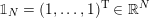
A matrix
 $P\in \mathbb{R}^{L\times M}$
is called bi-stochastic if all its entries are non-negative, which we will abbreviate by
$P\in \mathbb{R}^{L\times M}$
is called bi-stochastic if all its entries are non-negative, which we will abbreviate by
 $P\geq 0$
, and
$P\geq 0$
, and
 $$\begin{eqnarray}\mathop{\sum }_{l=1}^{L}q_{li}=p_{0},\quad \mathop{\sum }_{i=1}^{M}q_{li}=p_{1},\end{eqnarray}$$
where both
 $p_{1}\in \mathbb{R}^{L}$
and
$p_{1}\in \mathbb{R}^{L}$
and
 $p_{0}\in \mathbb{R}^{M}$
are probability vectors. A matrix
$p_{0}\in \mathbb{R}^{M}$
are probability vectors. A matrix
 $Q\in \mathbb{R}^{M\times M}$
defines a discrete Markov chain if all its entries are non-negative and
$Q\in \mathbb{R}^{M\times M}$
defines a discrete Markov chain if all its entries are non-negative and
 $$\begin{eqnarray}\mathop{\sum }_{l=1}^{L}q_{li}=1.\end{eqnarray}$$
The Kullback–Leibler divergence between two bi-stochastic matrices
 $P\in \mathbb{R}^{L\times M}$
and
$P\in \mathbb{R}^{L\times M}$
and
 $Q\in \mathbb{R}^{L\times M}$
is defined by
$Q\in \mathbb{R}^{L\times M}$
is defined by
 $$\begin{eqnarray}\text{KL}\,(P||Q):=\mathop{\sum }_{l,j}p_{lj}\log \displaystyle \frac{p_{lj}}{q_{lj}}.\end{eqnarray}$$
Here we have assumed for simplicity that
 $q_{lj}>0$
for all entries of
$q_{lj}>0$
for all entries of
 $Q$
. This definition extends to the Kullback–Leibler divergence between two discrete Markov chains.
$Q$
. This definition extends to the Kullback–Leibler divergence between two discrete Markov chains.
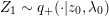
The transition probability going from state
 $z_{0}$
at time
$z_{0}$
at time
 $t=0$
to state
$t=0$
to state
 $z_{1}$
at time
$z_{1}$
at time
 $t=1$
is denoted by
$t=1$
is denoted by
 $q_{+}(z_{1}|z_{0})$
. Hence, given an initial PDF
$q_{+}(z_{1}|z_{0})$
. Hence, given an initial PDF
 $\unicode[STIX]{x1D70B}_{0}(z_{0})$
at
$\unicode[STIX]{x1D70B}_{0}(z_{0})$
at
 $t=0$
, the resulting (prediction or forecast) PDF at time
$t=0$
, the resulting (prediction or forecast) PDF at time
 $t=1$
is provided by
$t=1$
is provided by
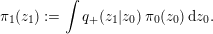 $$\begin{eqnarray}\unicode[STIX]{x1D70B}_{1}(z_{1}):=\int q_{+}(z_{1}|z_{0})\,\unicode[STIX]{x1D70B}_{0}(z_{0})\,\text{d}z_{0}.\end{eqnarray}$$
Given a twisting function
 $\unicode[STIX]{x1D713}(z)>0$
, the twisted transition kernel
$\unicode[STIX]{x1D713}(z)>0$
, the twisted transition kernel
 $q_{+}^{\unicode[STIX]{x1D713}}(z_{1}|z_{0})$
is defined by
$q_{+}^{\unicode[STIX]{x1D713}}(z_{1}|z_{0})$
is defined by
 $$\begin{eqnarray}q_{+}^{\unicode[STIX]{x1D713}}(z_{1}|z_{0}):=\unicode[STIX]{x1D713}(z_{1})\,q_{+}(z_{1}|z_{0})\,\widehat{\unicode[STIX]{x1D713}}(z_{0})^{-1}\end{eqnarray}$$
provided
 $$\begin{eqnarray}\widehat{\unicode[STIX]{x1D713}}(z_{0}):=\int q_{+}(z_{1}|z_{0})\,\unicode[STIX]{x1D713}(z_{1})\,\text{d}z_{1}\end{eqnarray}$$
is non-zero for all
 $z_{0}$
. See Definition 2.8 for more details.
$z_{0}$
. See Definition 2.8 for more details.
If transitions are characterized by a discrete Markov chain
 $Q_{+}\in \mathbb{R}^{M}$
, then a twisted Markov chain is provided by
$Q_{+}\in \mathbb{R}^{M}$
, then a twisted Markov chain is provided by
 $$\begin{eqnarray}Q_{+}^{u}=D(u)\,Q_{+}\,D(v)^{-1}\end{eqnarray}$$
for given twisting vector
 $u\in \mathbb{R}^{M}$
with positive entries
$u\in \mathbb{R}^{M}$
with positive entries
 $u_{i}$
, i.e.
$u_{i}$
, i.e.
 $u>0$
, and the vector
$u>0$
, and the vector
 $v\in \mathbb{R}^{M}$
determined by
$v\in \mathbb{R}^{M}$
determined by
 $$\begin{eqnarray}v=(D(u)\,Q_{+})^{\text{T}}\,\unicode[STIX]{x1D7D9}_{M}.\end{eqnarray}$$
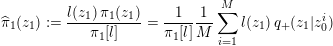
The conditional probability of observing
 $y$
given
$y$
given
 $z$
is denoted by
$z$
is denoted by
 $\unicode[STIX]{x1D70B}(y|z)$
and the likelihood of
$\unicode[STIX]{x1D70B}(y|z)$
and the likelihood of
 $z$
given an observed
$z$
given an observed
 $y$
is abbreviated by
$y$
is abbreviated by
 $l(z)=\unicode[STIX]{x1D70B}(y|z)$
. We will also use the abbreviations
$l(z)=\unicode[STIX]{x1D70B}(y|z)$
. We will also use the abbreviations
 $$\begin{eqnarray}\widehat{\unicode[STIX]{x1D70B}}_{1}(z_{1})=\unicode[STIX]{x1D70B}_{1}(z_{1}|y_{1})\end{eqnarray}$$
and
 $$\begin{eqnarray}\widehat{\unicode[STIX]{x1D70B}}_{0}(z_{0})=\unicode[STIX]{x1D70B}_{0}(z_{0}|y_{1})\end{eqnarray}$$
to denote the conditional PDFs of a process at time
 $t=1$
given data at time
$t=1$
given data at time
 $t=1$
(filtering) and the conditional PDF at time
$t=1$
(filtering) and the conditional PDF at time
 $t=0$
given data at time
$t=0$
given data at time
 $t=1$
(smoothing), respectively. Finally, we also introduce the evidence
$t=1$
(smoothing), respectively. Finally, we also introduce the evidence
 $$\begin{eqnarray}\unicode[STIX]{x1D6FD}:=\unicode[STIX]{x1D70B}_{1}[l]=\int p(y_{1}|z_{1})\unicode[STIX]{x1D70B}_{1}(z_{1})\,\text{d}z_{1}\end{eqnarray}$$
of observing
 $y_{1}$
under the given model as represented by the forecast PDF (1.1). A more precise definition of these expressions will be given in the following section.
$y_{1}$
under the given model as represented by the forecast PDF (1.1). A more precise definition of these expressions will be given in the following section.
2 Mathematical foundation of discrete-time DA
Let us assume that we are given partial and noisy observations
 $y_{k}$
,
$y_{k}$
,
 $k=1,\ldots ,K,$
of a stochastic process in regular time intervals of length
$k=1,\ldots ,K,$
of a stochastic process in regular time intervals of length
 $T=1$
. Given a likelihood function
$T=1$
. Given a likelihood function
 $\unicode[STIX]{x1D70B}(y|z)$
, a Markov transition kernel
$\unicode[STIX]{x1D70B}(y|z)$
, a Markov transition kernel
 $q_{+}(z^{\prime }|z)$
and an initial distribution
$q_{+}(z^{\prime }|z)$
and an initial distribution
 $\unicode[STIX]{x1D70B}_{0}$
, the associated prior and posterior PDFs are given by
$\unicode[STIX]{x1D70B}_{0}$
, the associated prior and posterior PDFs are given by
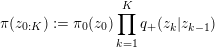 $$\begin{eqnarray}\unicode[STIX]{x1D70B}(z_{0:K}):=\unicode[STIX]{x1D70B}_{0}(z_{0})\mathop{\prod }_{k=1}^{K}q_{+}(z_{k}|z_{k-1})\end{eqnarray}$$
and
 $$\begin{eqnarray}\unicode[STIX]{x1D70B}(z_{0:K}|y_{1:K}):=\displaystyle \frac{\unicode[STIX]{x1D70B}_{0}(z_{0})\mathop{\prod }_{k=1}^{K}\unicode[STIX]{x1D70B}(y_{k}|z_{k})\,q_{+}(z_{k}|z_{k-1})}{\unicode[STIX]{x1D70B}(y_{1:K})},\end{eqnarray}$$
respectively (Jazwinski Reference Jazwinski1970, Särkkä Reference Särkkä2013). While it is of broad interest to approximate the posterior or smoothing PDF (2.2), we will focus on the recursive approximation of the filtering PDFs
 $\unicode[STIX]{x1D70B}(z_{k}|y_{1:k})$
using sequential particle filters in this paper. More specifically, we wish to address the following computational task.
$\unicode[STIX]{x1D70B}(z_{k}|y_{1:k})$
using sequential particle filters in this paper. More specifically, we wish to address the following computational task.
Problem 2.1. We have
 $M$
equally weighted Monte Carlo samples
$M$
equally weighted Monte Carlo samples
 $z_{k-1}^{i}$
,
$z_{k-1}^{i}$
,
 $i=1,\ldots ,M$
, from the filtering PDF
$i=1,\ldots ,M$
, from the filtering PDF
 $\unicode[STIX]{x1D70B}(z_{k-1}|y_{1:k-1})$
at time
$\unicode[STIX]{x1D70B}(z_{k-1}|y_{1:k-1})$
at time
 $t=k-1$
available and we wish to produce
$t=k-1$
available and we wish to produce
 $M$
equally weighted samples from the filtering PDF
$M$
equally weighted samples from the filtering PDF
 $\unicode[STIX]{x1D70B}(z_{k}|y_{1:k})$
at time
$\unicode[STIX]{x1D70B}(z_{k}|y_{1:k})$
at time
 $t=k$
having access to the transition kernel
$t=k$
having access to the transition kernel
 $q_{+}(z_{k}|z_{k-1})$
and the likelihood
$q_{+}(z_{k}|z_{k-1})$
and the likelihood
 $\unicode[STIX]{x1D70B}(y_{k}|z_{k})$
only. Since the computational task is exactly the same for all indices
$\unicode[STIX]{x1D70B}(y_{k}|z_{k})$
only. Since the computational task is exactly the same for all indices
 $k\geq 1$
, we simply set
$k\geq 1$
, we simply set
 $k=1$
throughout this paper.
$k=1$
throughout this paper.
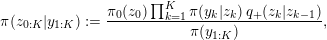
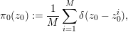
We introduce some notations before we discuss several possibilities of addressing Problem 2.1. Since we do not have direct access to the filtering distribution at time
 $k=0$
, the PDF at
$k=0$
, the PDF at
 $t_{0}$
becomes
$t_{0}$
becomes
 $$\begin{eqnarray}\unicode[STIX]{x1D70B}_{0}(z_{0}):=\displaystyle \frac{1}{M}\mathop{\sum }_{i=1}^{M}\unicode[STIX]{x1D6FF}(z_{0}-z_{0}^{i}),\end{eqnarray}$$
where
 $\unicode[STIX]{x1D6FF}(z)$
denotes the Dirac delta function and
$\unicode[STIX]{x1D6FF}(z)$
denotes the Dirac delta function and
 $z_{0}^{i}$
,
$z_{0}^{i}$
,
 $i=1,\ldots ,M$
, are
$i=1,\ldots ,M$
, are
 $M$
given Monte Carlo samples representing the actual filtering distribution. Recall that we abbreviate the resulting filtering PDF
$M$
given Monte Carlo samples representing the actual filtering distribution. Recall that we abbreviate the resulting filtering PDF
 $\unicode[STIX]{x1D70B}(z_{1}|y_{1})$
at
$\unicode[STIX]{x1D70B}(z_{1}|y_{1})$
at
 $t=1$
by
$t=1$
by
 $\widehat{\unicode[STIX]{x1D70B}}_{1}(z_{1})$
and the likelihood
$\widehat{\unicode[STIX]{x1D70B}}_{1}(z_{1})$
and the likelihood
 $\unicode[STIX]{x1D70B}(y_{1}|z_{1})$
by
$\unicode[STIX]{x1D70B}(y_{1}|z_{1})$
by
 $l(z_{1})$
. Because of (1.1), the forecast PDF is given by
$l(z_{1})$
. Because of (1.1), the forecast PDF is given by
 $$\begin{eqnarray}\unicode[STIX]{x1D70B}_{1}(z_{1})=\displaystyle \frac{1}{M}\mathop{\sum }_{i=1}^{M}q_{+}(z_{1}|z_{0}^{i})\end{eqnarray}$$
and the filtering PDF at time
 $t=1$
by
$t=1$
by
 $$\begin{eqnarray}\widehat{\unicode[STIX]{x1D70B}}_{1}(z_{1}):=\displaystyle \frac{l(z_{1})\,\unicode[STIX]{x1D70B}_{1}(z_{1})}{\unicode[STIX]{x1D70B}_{1}[l]}=\displaystyle \frac{1}{\unicode[STIX]{x1D70B}_{1}[l]}\displaystyle \frac{1}{M}\mathop{\sum }_{i=1}^{M}l(z_{1})\,q_{+}(z_{1}|z_{0}^{i})\end{eqnarray}$$
according to Bayes’ theorem.
Remark 2.2. The normalization constant
 $\unicode[STIX]{x1D70B}(y_{1:K})$
in (2.2), also called the evidence, can be determined recursively using
$\unicode[STIX]{x1D70B}(y_{1:K})$
in (2.2), also called the evidence, can be determined recursively using
 $$\begin{eqnarray}\displaystyle \unicode[STIX]{x1D70B}(y_{1:k}) & = & \displaystyle \unicode[STIX]{x1D70B}(y_{1:k-1})\,\int \unicode[STIX]{x1D70B}(y_{k},z_{k-1})\,\unicode[STIX]{x1D70B}(z_{k-1}|y_{1:k-1})\,\text{d}z_{k-1}\nonumber\\ \displaystyle & = & \displaystyle \unicode[STIX]{x1D70B}(y_{1:k-1})\,\int \int \unicode[STIX]{x1D70B}(y_{k}|z_{k})\,q_{+}(z_{k}|z_{k-1})\,\unicode[STIX]{x1D70B}(z_{k-1}|y_{1:k-1})\,\text{d}z_{k-1}\,\text{d}z_{k}\nonumber\\ \displaystyle & = & \displaystyle \unicode[STIX]{x1D70B}(y_{1:k-1})\,\int \unicode[STIX]{x1D70B}(y_{k}|z_{k})\,\unicode[STIX]{x1D70B}(z_{k}|y_{1:k-1})\,\text{d}z_{k}\end{eqnarray}$$
(Särkkä Reference Särkkä2013, Reich and Cotter Reference Reich and Cotter2015). Since, as for the state estimation problem, the computational task is the same for each index
 $k\geq 1$
, we simply set
$k\geq 1$
, we simply set
 $k=1$
and formally use
$k=1$
and formally use
 $\unicode[STIX]{x1D70B}(y_{1:0})\equiv 1$
. We are then left with
$\unicode[STIX]{x1D70B}(y_{1:0})\equiv 1$
. We are then left with
 $$\begin{eqnarray}\unicode[STIX]{x1D6FD}:=\unicode[STIX]{x1D70B}_{1}[l]=\displaystyle \frac{1}{M}\mathop{\sum }_{i=1}^{M}\int l(z_{1})\,q_{+}(z_{1}|z_{0}^{i})\,\text{d}z_{1}\end{eqnarray}$$
within the setting of Problem 2.1, and
 $\unicode[STIX]{x1D6FD}$
becomes a shorthand for
$\unicode[STIX]{x1D6FD}$
becomes a shorthand for
 $\unicode[STIX]{x1D70B}(y_{1})$
. If the model depends on parameters,
$\unicode[STIX]{x1D70B}(y_{1})$
. If the model depends on parameters,
 $\unicode[STIX]{x1D706}$
, or different models are to be compared, then it is important to evaluate the evidence (2.7) for each parameter value
$\unicode[STIX]{x1D706}$
, or different models are to be compared, then it is important to evaluate the evidence (2.7) for each parameter value
 $\unicode[STIX]{x1D706}$
or model, respectively. More specifically, if
$\unicode[STIX]{x1D706}$
or model, respectively. More specifically, if
 $q_{+}(z_{1}|z_{0};\unicode[STIX]{x1D706})$
, then
$q_{+}(z_{1}|z_{0};\unicode[STIX]{x1D706})$
, then
 $\unicode[STIX]{x1D6FD}=\unicode[STIX]{x1D6FD}(\unicode[STIX]{x1D706})$
in (2.7) and larger values of
$\unicode[STIX]{x1D6FD}=\unicode[STIX]{x1D6FD}(\unicode[STIX]{x1D706})$
in (2.7) and larger values of
 $\unicode[STIX]{x1D6FD}(\unicode[STIX]{x1D706})$
indicate a better fit of the transition kernel to the data for that parameter value. One can then perform Bayesian parameter inference based upon appropriate approximations to the likelihood
$\unicode[STIX]{x1D6FD}(\unicode[STIX]{x1D706})$
indicate a better fit of the transition kernel to the data for that parameter value. One can then perform Bayesian parameter inference based upon appropriate approximations to the likelihood
 $\unicode[STIX]{x1D70B}(y_{1}|\unicode[STIX]{x1D706})=\unicode[STIX]{x1D6FD}(\unicode[STIX]{x1D706})$
and a given prior PDF
$\unicode[STIX]{x1D70B}(y_{1}|\unicode[STIX]{x1D706})=\unicode[STIX]{x1D6FD}(\unicode[STIX]{x1D706})$
and a given prior PDF
 $\unicode[STIX]{x1D70B}(\unicode[STIX]{x1D706})$
. The extension to the complete data set
$\unicode[STIX]{x1D70B}(\unicode[STIX]{x1D706})$
. The extension to the complete data set
 $y_{1:K}$
,
$y_{1:K}$
,
 $K>1$
, is straightforward using (2.6) and an appropriate data assimilation algorithm, i.e. algorithms that can tackle Problem 2.1 sequentially.
$K>1$
, is straightforward using (2.6) and an appropriate data assimilation algorithm, i.e. algorithms that can tackle Problem 2.1 sequentially.
Alternatively, one can treat a combined state–parameter estimation problem as a particular case of Problem 2.1 by introducing the extended state variable
 $(z,\unicode[STIX]{x1D706})$
and augmented transition probabilities
$(z,\unicode[STIX]{x1D706})$
and augmented transition probabilities
 $Z_{1}\sim q_{+}(\cdot |z_{0},\unicode[STIX]{x1D706}_{0})$
and
$Z_{1}\sim q_{+}(\cdot |z_{0},\unicode[STIX]{x1D706}_{0})$
and
 $\mathbb{P}[\unicode[STIX]{x1D6EC}_{1}=\unicode[STIX]{x1D706}_{0}]=1$
. The state augmentation technique allows one to extend all approaches discussed in this paper for Problem 2.1 to combined state–parameter estimation.
$\mathbb{P}[\unicode[STIX]{x1D6EC}_{1}=\unicode[STIX]{x1D706}_{0}]=1$
. The state augmentation technique allows one to extend all approaches discussed in this paper for Problem 2.1 to combined state–parameter estimation.
See Kantas et al. (Reference Kantas, Doucet, Singh, Maciejowski and Chopin2015) for a detailed survey of the topic of combined state and parameter estimation.
The filtering distribution
 $\widehat{\unicode[STIX]{x1D70B}}_{1}$
at time
$\widehat{\unicode[STIX]{x1D70B}}_{1}$
at time
 $t=1$
implies a smoothing distribution at time
$t=1$
implies a smoothing distribution at time
 $t=0$
, which is given by
$t=0$
, which is given by
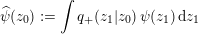
 $$\begin{eqnarray}\widehat{\unicode[STIX]{x1D70B}}_{0}(z_{0}):=\displaystyle \frac{1}{\unicode[STIX]{x1D6FD}}\int l(z_{1})\,q_{+}(z_{1}|z_{0})\,\unicode[STIX]{x1D70B}_{0}(z_{0})\,\text{d}z_{1}=\displaystyle \frac{1}{M}\mathop{\sum }_{i=1}^{M}\unicode[STIX]{x1D6FE}^{i}\unicode[STIX]{x1D6FF}(z_{0}-z_{0}^{i})\end{eqnarray}$$
with weights
 $$\begin{eqnarray}\unicode[STIX]{x1D6FE}^{i}:=\displaystyle \frac{1}{\unicode[STIX]{x1D6FD}}\int l(z_{1})\,q_{+}(z_{1}|z_{0}^{i})\,\text{d}z_{1}.\end{eqnarray}$$
It is important to note that the filtering PDF
 $\widehat{\unicode[STIX]{x1D70B}}_{1}$
can be obtained from
$\widehat{\unicode[STIX]{x1D70B}}_{1}$
can be obtained from
 $\widehat{\unicode[STIX]{x1D70B}}_{0}$
using the transition kernels
$\widehat{\unicode[STIX]{x1D70B}}_{0}$
using the transition kernels
 $$\begin{eqnarray}\widehat{q}_{+}(z_{1}|z_{0}^{i}):=\displaystyle \frac{l(z_{1})\,q_{+}(z_{1}|z_{0}^{i})}{\unicode[STIX]{x1D6FD}\,\unicode[STIX]{x1D6FE}^{i}},\end{eqnarray}$$
that is,
 $$\begin{eqnarray}\widehat{\unicode[STIX]{x1D70B}}_{1}(z_{1})=\displaystyle \frac{1}{M}\mathop{\sum }_{i=1}^{M}\widehat{q}_{+}(z_{1}|z_{0}^{i})\,\unicode[STIX]{x1D6FE}^{i}.\end{eqnarray}$$
See Figure 2.1 for a schematic illustration of these distributions and their mutual relationships.
Remark 2.3. The modified transition kernel (2.10) can be seen as a particular instance of a twisted transition kernel (1.2) with
 $\unicode[STIX]{x1D713}(z)=l(z)/\unicode[STIX]{x1D6FD}$
and
$\unicode[STIX]{x1D713}(z)=l(z)/\unicode[STIX]{x1D6FD}$
and
 $\widehat{\unicode[STIX]{x1D713}}(z_{0}^{i})=\unicode[STIX]{x1D6FE}^{i}$
. Such twisting kernels will play a prominent role in this survey, not only in the context of optimal proposals (Doucet et al.
Reference Doucet, de Freitas and Gordon2001, Arulampalam, Maskell, Gordon and Clapp Reference Arulampalam, Maskell, Gordon and Clapp2002) but also in the context of the Schrödinger approach to data assimilation, i.e. scenario (C) below.
$\widehat{\unicode[STIX]{x1D713}}(z_{0}^{i})=\unicode[STIX]{x1D6FE}^{i}$
. Such twisting kernels will play a prominent role in this survey, not only in the context of optimal proposals (Doucet et al.
Reference Doucet, de Freitas and Gordon2001, Arulampalam, Maskell, Gordon and Clapp Reference Arulampalam, Maskell, Gordon and Clapp2002) but also in the context of the Schrödinger approach to data assimilation, i.e. scenario (C) below.
The following scenarios of how to tackle Problem 2.1, that is, how to produce the desired samples
 $\widehat{z}_{1}^{i}$
,
$\widehat{z}_{1}^{i}$
,
 $i=1,\ldots ,M$
, from the filtering PDF (2.5), will be considered in this paper.
$i=1,\ldots ,M$
, from the filtering PDF (2.5), will be considered in this paper.
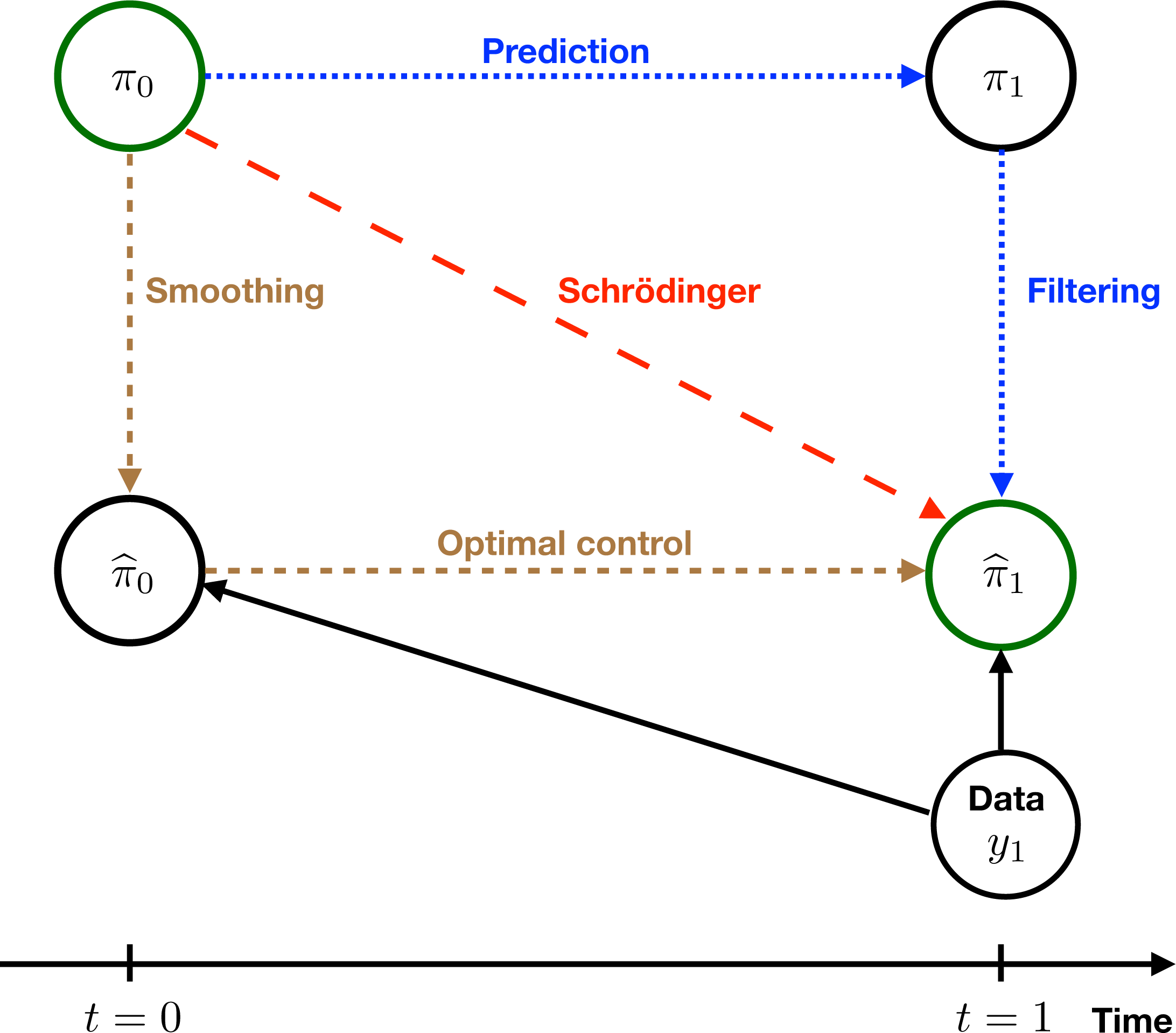
Figure 2.1. Schematic illustration of a single data assimilation cycle. The distribution
 $\unicode[STIX]{x1D70B}_{0}$
characterizes the distribution of states conditioned on all observations up to and including
$\unicode[STIX]{x1D70B}_{0}$
characterizes the distribution of states conditioned on all observations up to and including
 $t_{0}$
, which we set here to
$t_{0}$
, which we set here to
 $t=0$
for simplicity. The predictive distribution at time
$t=0$
for simplicity. The predictive distribution at time
 $t_{1}=1$
, as generated by the model dynamics, is denoted by
$t_{1}=1$
, as generated by the model dynamics, is denoted by
 $\unicode[STIX]{x1D70B}_{1}$
. Upon assimilation of the data
$\unicode[STIX]{x1D70B}_{1}$
. Upon assimilation of the data
 $y_{1}$
and application of Bayes’ formula, one obtains the filtering distribution
$y_{1}$
and application of Bayes’ formula, one obtains the filtering distribution
 $\widehat{\unicode[STIX]{x1D70B}}_{1}$
. The conditional distribution of states at time
$\widehat{\unicode[STIX]{x1D70B}}_{1}$
. The conditional distribution of states at time
 $t_{0}$
conditioned on all the available data including
$t_{0}$
conditioned on all the available data including
 $y_{1}$
is denoted by
$y_{1}$
is denoted by
 $\widehat{\unicode[STIX]{x1D70B}}_{0}$
. Control theory provides the adjusted model dynamics for transforming
$\widehat{\unicode[STIX]{x1D70B}}_{0}$
. Control theory provides the adjusted model dynamics for transforming
 $\widehat{\unicode[STIX]{x1D70B}}_{0}$
into
$\widehat{\unicode[STIX]{x1D70B}}_{0}$
into
 $\widehat{\unicode[STIX]{x1D70B}}_{1}$
. Finally, the Schrödinger problem links
$\widehat{\unicode[STIX]{x1D70B}}_{1}$
. Finally, the Schrödinger problem links
 $\unicode[STIX]{x1D70B}_{0}$
and
$\unicode[STIX]{x1D70B}_{0}$
and
 $\widehat{\unicode[STIX]{x1D70B}}_{1}$
in the form of a penalized boundary value problem in the space of joint probability measures. Data assimilation scenario (A) corresponds to the dotted lines, scenario (B) to the short-dashed lines, and scenario (C) to the long-dashed line.
$\widehat{\unicode[STIX]{x1D70B}}_{1}$
in the form of a penalized boundary value problem in the space of joint probability measures. Data assimilation scenario (A) corresponds to the dotted lines, scenario (B) to the short-dashed lines, and scenario (C) to the long-dashed line.
Definition 2.4. We define the following three scenarios of how to tackle Problem 2.1.
(A) We first produce samples,
 $z_{1}^{i}$
, from the forecast PDF
$\unicode[STIX]{x1D70B}_{1}$
and then transform those samples into samples,
$\widehat{z}_{1}^{i}$
, from
$\widehat{\unicode[STIX]{x1D70B}}_{1}$
. This can be viewed as introducing a Markov transition kernel
$q_{1}(\widehat{z}_{1}|z_{1})$
with the property that (2.11)Techniques from optimal transportation can be used to find appropriate transition kernels (Villani Reference Villani2003, Reference Villani2009, Reich and Cotter Reference Reich and Cotter2015).$$\begin{eqnarray}\widehat{\unicode[STIX]{x1D70B}}_{1}(\widehat{z}_{1})=\int q_{1}(\widehat{z}_{1}|z_{1})\,\unicode[STIX]{x1D70B}_{1}(z_{1})\,\text{d}z_{1}.\end{eqnarray}$$
$z_{1}^{i}$
, from the forecast PDF
$\unicode[STIX]{x1D70B}_{1}$
and then transform those samples into samples,
$\widehat{z}_{1}^{i}$
, from
$\widehat{\unicode[STIX]{x1D70B}}_{1}$
. This can be viewed as introducing a Markov transition kernel
$q_{1}(\widehat{z}_{1}|z_{1})$
with the property that (2.11)Techniques from optimal transportation can be used to find appropriate transition kernels (Villani Reference Villani2003, Reference Villani2009, Reich and Cotter Reference Reich and Cotter2015).$$\begin{eqnarray}\widehat{\unicode[STIX]{x1D70B}}_{1}(\widehat{z}_{1})=\int q_{1}(\widehat{z}_{1}|z_{1})\,\unicode[STIX]{x1D70B}_{1}(z_{1})\,\text{d}z_{1}.\end{eqnarray}$$
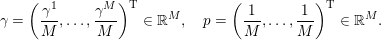
(B) We first produce
$M$
samples from the smoothing PDF (2.8) via resampling with replacement and then sample from
$\widehat{\unicode[STIX]{x1D70B}}_{1}$
using the smoothing transition kernels (2.10). The resampling can be represented in terms of a Markov transition matrix
$Q_{0}\in \mathbb{R}^{M\times M}$
such that Here we have introduced the associated probability vectors$$\begin{eqnarray}\unicode[STIX]{x1D6FE}=Q_{0}\,p.\end{eqnarray}$$
(2.12)Techniques from optimal transport will be explored to find such Markov transition matrices in Section 3.$$\begin{eqnarray}\unicode[STIX]{x1D6FE}=\biggl(\displaystyle \frac{\unicode[STIX]{x1D6FE}^{1}}{M},\ldots ,\displaystyle \frac{\unicode[STIX]{x1D6FE}^{M}}{M}\biggr)^{\text{T}}\in \mathbb{R}^{M},\quad p=\biggl(\displaystyle \frac{1}{M},\ldots ,\displaystyle \frac{1}{M}\biggr)^{\text{T}}\in \mathbb{R}^{M}.\end{eqnarray}$$
(C) We directly seek Markov transition kernels
$q_{+}^{\ast }(z_{1}|z_{0}^{i})$
,
$i=1,\ldots ,M$
, with the property that (2.13)and then draw a single sample,$$\begin{eqnarray}\widehat{\unicode[STIX]{x1D70B}}_{1}(z_{1})=\displaystyle \frac{1}{M}\mathop{\sum }_{i=1}^{M}q_{+}^{\ast }(z_{1}|z_{0}^{i})\end{eqnarray}$$
$\widehat{z}_{1}^{i}$
, from each kernel
$q_{+}^{\ast }(z_{1}|z_{0}^{i})$
. Such kernels can be found by solving a Schrödinger problem (Leonard Reference Leonard2014, Chen et al.
Reference Chen, Georgiou and Pavon2014) as demonstrated in Section 2.3.


Scenario (A) forms the basis of the classical bootstrap particle filter (Doucet et al.
Reference Doucet, de Freitas and Gordon2001, Liu Reference Liu2001, Bain and Crisan Reference Bain and Crisan2008, Arulampalam et al.
Reference Arulampalam, Maskell, Gordon and Clapp2002) and also provides the starting point for many currently used ensemble-based data assimilation algorithms (Evensen Reference Evensen2006, Reich and Cotter Reference Reich and Cotter2015, Law et al.
Reference Law, Stuart and Zygalakis2015). Scenario (B) is also well known in the context of particle filters under the notion of optimal proposal densities (Doucet et al.
Reference Doucet, de Freitas and Gordon2001, Arulampalam et al.
Reference Arulampalam, Maskell, Gordon and Clapp2002, Fearnhead and Künsch Reference Fearnhead and Künsch2018). Recently there has been renewed interest in scenario (B) from the perspective of optimal control and twisting approaches (Guarniero, Johansen and Lee Reference Guarniero, Johansen and Lee2017, Heng, Bishop, Deligiannidis and Doucet Reference Heng, Bishop, Deligiannidis and Doucet2018, Kappen and Ruiz Reference Kappen and Ruiz2016, Ruiz and Kappen Reference Ruiz and Kappen2017). Finally, scenario (C) has not yet been explored in the context of particle filters and data assimilation, primarily because the required kernels
 $q_{+}^{\ast }$
are typically not available in closed form or cannot be easily sampled from. However, as we will argue in this paper, progress on the numerical solution of Schrödinger’s problem (Cuturi Reference Cuturi and Burges2013, Peyre and Cuturi Reference Peyre and Cuturi2018) turns scenario (C) into a viable option in addition to providing a unifying mathematical framework for data assimilation.
$q_{+}^{\ast }$
are typically not available in closed form or cannot be easily sampled from. However, as we will argue in this paper, progress on the numerical solution of Schrödinger’s problem (Cuturi Reference Cuturi and Burges2013, Peyre and Cuturi Reference Peyre and Cuturi2018) turns scenario (C) into a viable option in addition to providing a unifying mathematical framework for data assimilation.
We emphasize that not all existing particle methods fit into these three scenarios. For example, the methods put forward by van Leeuwen (Reference van Leeuwen and van Leeuwen2015) are based on proposal densities which attempt to overcome limitations of scenario (B) and which lead to less variable particle weights, thus attempting to obtain particle filter implementations closer to what we denote here as scenario (C). More broadly speaking, the exploration of alternative proposal densities in the context of data assimilation has started only recently. See, for example, Vanden-Eijnden and Weare (Reference Vanden-Eijnden and Weare2012), Morzfeld, Tu, Atkins and Chorin (Reference Morzfeld, Tu, Atkins and Chorin2012), van Leeuwen (Reference van Leeuwen and van Leeuwen2015), Pons Llopis, Kantas, Beskos and Jasra (Reference Pons Llopis, Kantas, Beskos and Jasra2018) and van Leeuwen et al. (Reference van Leeuwen, Künsch, Nerger, Potthast and Reich2018).
The accuracy of an ensemble-based data assimilation method can be characterized in terms of its effective sample size
 $M_{\text{eff}}$
(Liu Reference Liu2001). The relevant effective sample size for scenario (B) is, for example, given by
$M_{\text{eff}}$
(Liu Reference Liu2001). The relevant effective sample size for scenario (B) is, for example, given by
 $$\begin{eqnarray}M_{\text{eff}}=\displaystyle \frac{M^{2}}{\mathop{\sum }_{i=1}^{M}(\unicode[STIX]{x1D6FE}^{i})^{2}}=\displaystyle \frac{1}{\Vert \unicode[STIX]{x1D6FE}\Vert ^{2}}.\end{eqnarray}$$
We find that
 $M\geq M_{\text{eff}}\geq 1$
and the accuracy of a data assimilation step decreases with decreasing
$M\geq M_{\text{eff}}\geq 1$
and the accuracy of a data assimilation step decreases with decreasing
 $M_{\text{eff}}$
, that is, the convergence rate
$M_{\text{eff}}$
, that is, the convergence rate
 $1/\sqrt{M}$
of a standard Monte Carlo method is replaced by
$1/\sqrt{M}$
of a standard Monte Carlo method is replaced by
 $1/\sqrt{M_{\text{e ff }}}$
(Agapiou, Papaspipliopoulos, Sanz-Alonso and Stuart Reference Agapiou, Papaspipliopoulos, Sanz-Alonso and Stuart2017). Scenario (C) offers a route around this problem by bridging
$1/\sqrt{M_{\text{e ff }}}$
(Agapiou, Papaspipliopoulos, Sanz-Alonso and Stuart Reference Agapiou, Papaspipliopoulos, Sanz-Alonso and Stuart2017). Scenario (C) offers a route around this problem by bridging
 $\unicode[STIX]{x1D70B}_{0}$
with
$\unicode[STIX]{x1D70B}_{0}$
with
 $\widehat{\unicode[STIX]{x1D70B}}_{1}$
directly, that is, solving the Schrödinger problem delivers the best possible proposal densities leading to equally weighted particles without the need for resampling.Footnote
1
$\widehat{\unicode[STIX]{x1D70B}}_{1}$
directly, that is, solving the Schrödinger problem delivers the best possible proposal densities leading to equally weighted particles without the need for resampling.Footnote
1
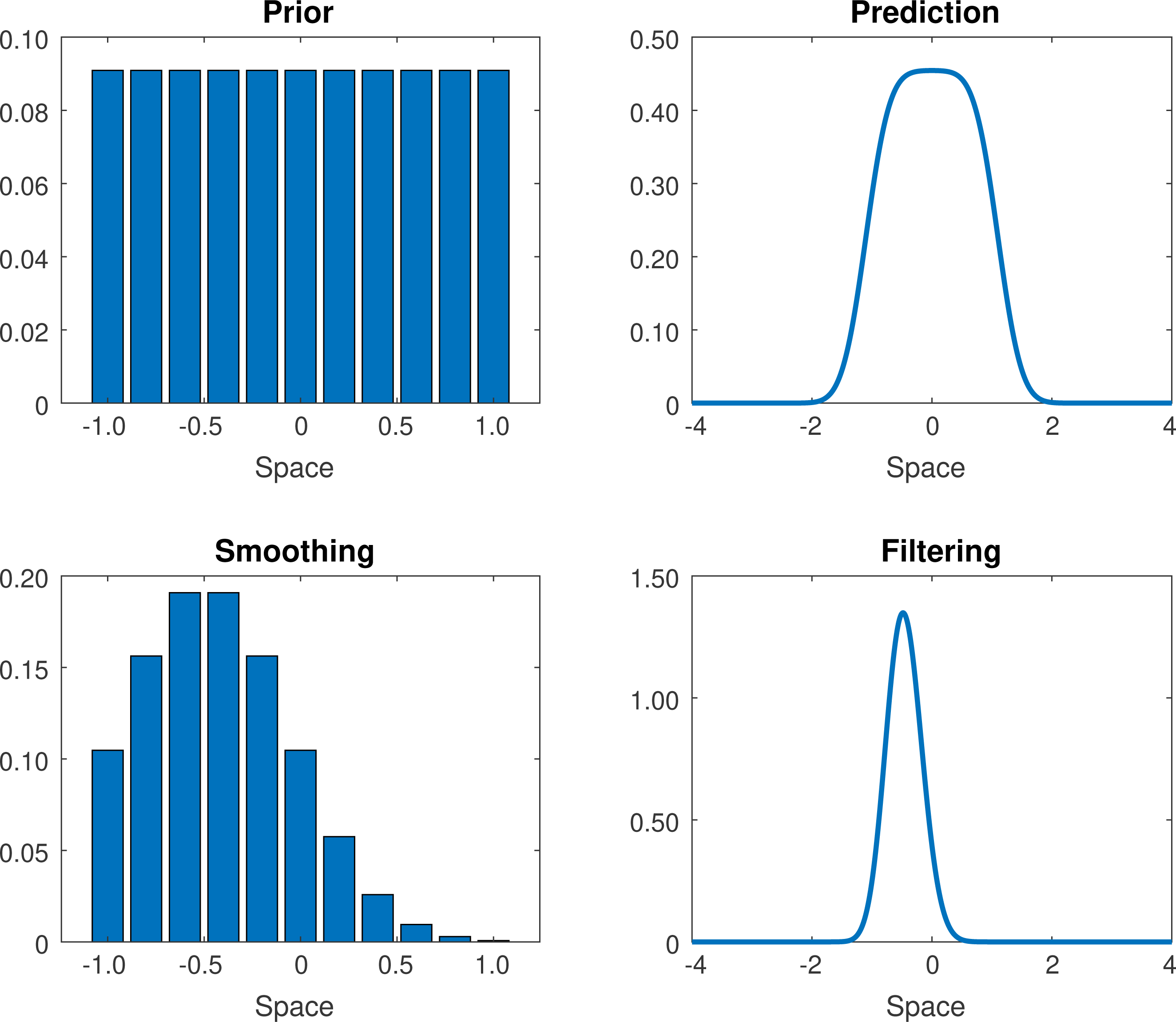
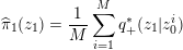
Figure 2.2. The initial PDF
 $\unicode[STIX]{x1D70B}_{0}$
, the forecast PDF
$\unicode[STIX]{x1D70B}_{0}$
, the forecast PDF
 $\unicode[STIX]{x1D70B}_{1}$
, the filtering PDF
$\unicode[STIX]{x1D70B}_{1}$
, the filtering PDF
 $\widehat{\unicode[STIX]{x1D70B}}_{1}$
, and the smoothing PDF
$\widehat{\unicode[STIX]{x1D70B}}_{1}$
, and the smoothing PDF
 $\widehat{\unicode[STIX]{x1D70B}}_{0}$
for a simple Gaussian transition kernel.
$\widehat{\unicode[STIX]{x1D70B}}_{0}$
for a simple Gaussian transition kernel.
Example 2.5. We illustrate the three scenarios with a simple example. The prior samples are given by
 $M=11$
equally spaced particles
$M=11$
equally spaced particles
 $z_{0}^{i}\in \mathbb{R}$
from the interval
$z_{0}^{i}\in \mathbb{R}$
from the interval
 $[-1,1]$
. The forecast PDF
$[-1,1]$
. The forecast PDF
 $\unicode[STIX]{x1D70B}_{1}$
is provided by
$\unicode[STIX]{x1D70B}_{1}$
is provided by
 $$\begin{eqnarray}\unicode[STIX]{x1D70B}_{1}(z)=\displaystyle \frac{1}{M}\mathop{\sum }_{i=1}^{M}\displaystyle \frac{1}{(2\unicode[STIX]{x1D70B})^{1/2}\unicode[STIX]{x1D70E}}\exp \biggl(-\displaystyle \frac{1}{2\unicode[STIX]{x1D70E}^{2}}(z-z_{0}^{i})^{2}\biggr)\end{eqnarray}$$
with variance
 $\unicode[STIX]{x1D70E}^{2}=0.1$
. The likelihood function is given by
$\unicode[STIX]{x1D70E}^{2}=0.1$
. The likelihood function is given by
 $$\begin{eqnarray}\unicode[STIX]{x1D70B}(y_{1}|z)=\displaystyle \frac{1}{(2\unicode[STIX]{x1D70B}R)^{1/2}}\exp \biggl(-\displaystyle \frac{1}{2R}(y_{1}-z)^{2}\biggr)\end{eqnarray}$$
with
 $R=0.1$
and
$R=0.1$
and
 $y_{1}=-0.5$
. The implied filtering and smoothing distributions can be found in Figure 2.2. Since
$y_{1}=-0.5$
. The implied filtering and smoothing distributions can be found in Figure 2.2. Since
 $\widehat{\unicode[STIX]{x1D70B}}_{1}$
is in the form of a weighted Gaussian mixture distribution, the Markov chain leading from
$\widehat{\unicode[STIX]{x1D70B}}_{1}$
is in the form of a weighted Gaussian mixture distribution, the Markov chain leading from
 $\widehat{\unicode[STIX]{x1D70B}}_{0}$
to
$\widehat{\unicode[STIX]{x1D70B}}_{0}$
to
 $\widehat{\unicode[STIX]{x1D70B}}_{1}$
can be stated explicitly, that is, (2.10) is provided by
$\widehat{\unicode[STIX]{x1D70B}}_{1}$
can be stated explicitly, that is, (2.10) is provided by
 $$\begin{eqnarray}\widehat{q}_{+}(z_{1}|z_{0}^{i})=\displaystyle \frac{1}{(2\unicode[STIX]{x1D70B})^{1/2}\widehat{\unicode[STIX]{x1D70E}}}\exp \biggl(-\displaystyle \frac{1}{2\widehat{\unicode[STIX]{x1D70E}}^{2}}(\bar{z}_{1}^{i}-z_{1})^{2}\biggr)\end{eqnarray}$$
with
 $$\begin{eqnarray}\widehat{\unicode[STIX]{x1D70E}}^{2}=\unicode[STIX]{x1D70E}^{2}-\displaystyle \frac{\unicode[STIX]{x1D70E}^{4}}{\unicode[STIX]{x1D70E}^{2}+R},\quad \bar{z}_{1}^{i}=z_{0}^{i}-\displaystyle \frac{\unicode[STIX]{x1D70E}^{2}}{\unicode[STIX]{x1D70E}^{2}+R}(z_{0}^{i}-y_{1}).\end{eqnarray}$$
The resulting transition kernels are displayed in Figure 2.3 together with the corresponding transition kernels for the Schrödinger approach, which connects
 $\unicode[STIX]{x1D70B}_{0}$
directly with
$\unicode[STIX]{x1D70B}_{0}$
directly with
 $\widehat{\unicode[STIX]{x1D70B}}_{1}$
.
$\widehat{\unicode[STIX]{x1D70B}}_{1}$
.
Figure 2.3. (a) The transition kernels (2.14) for the
 $M=11$
different particles
$M=11$
different particles
 $z_{0}^{i}$
. These correspond to the optimal control path in Figure 2.1. (b) The corresponding transition kernels, which lead directly from
$z_{0}^{i}$
. These correspond to the optimal control path in Figure 2.1. (b) The corresponding transition kernels, which lead directly from
 $\unicode[STIX]{x1D70B}_{0}$
to
$\unicode[STIX]{x1D70B}_{0}$
to
 $\widehat{\unicode[STIX]{x1D70B}}_{1}$
. These correspond to the Schrödinger path in Figure 2.1. Details of how to compute these Schrödinger transition kernels,
$\widehat{\unicode[STIX]{x1D70B}}_{1}$
. These correspond to the Schrödinger path in Figure 2.1. Details of how to compute these Schrödinger transition kernels,
 $q_{+}^{\ast }(z_{1}|z_{0}^{i})$
, can be found in Section 3.4.1.
$q_{+}^{\ast }(z_{1}|z_{0}^{i})$
, can be found in Section 3.4.1.
Remark 2.6. It is often assumed in optimal control or rare event simulations arising from statistical mechanics that
 $\unicode[STIX]{x1D70B}_{0}$
in (2.1) is a point measure, that is, the starting point of the simulation is known exactly. See, for example, Hartmann, Richter, Schütte and Zhang (Reference Hartmann, Richter, Schütte and Zhang2017). This corresponds to (2.3) with
$\unicode[STIX]{x1D70B}_{0}$
in (2.1) is a point measure, that is, the starting point of the simulation is known exactly. See, for example, Hartmann, Richter, Schütte and Zhang (Reference Hartmann, Richter, Schütte and Zhang2017). This corresponds to (2.3) with
 $M=1$
. It turns out that the associated smoothing problem becomes equivalent to Schrödinger’s problem under this particular setting since the distribution at
$M=1$
. It turns out that the associated smoothing problem becomes equivalent to Schrödinger’s problem under this particular setting since the distribution at
 $t=0$
is fixed.
$t=0$
is fixed.
The remainder of this section is structured as follows. We first recapitulate the pure prediction problem for discrete-time Markov processes and continuous-time diffusion processes, after which we discuss the filtering and smoothing problem for a single data assimilation step as relevant for scenarios (A) and (B). The final subsection is devoted to the Schrödinger problem (Leonard Reference Leonard2014, Chen et al.
Reference Chen, Georgiou and Pavon2014) of bridging the filtering distribution,
 $\unicode[STIX]{x1D70B}_{0}$
, at
$\unicode[STIX]{x1D70B}_{0}$
, at
 $t=0$
directly with the filtering distribution,
$t=0$
directly with the filtering distribution,
 $\widehat{\unicode[STIX]{x1D70B}}_{1}$
, at
$\widehat{\unicode[STIX]{x1D70B}}_{1}$
, at
 $t=1$
, thus leading to scenario (C).
$t=1$
, thus leading to scenario (C).
2.1 Prediction
We assume under the chosen computational setting that we have access to
 $M$
samples
$M$
samples
 $z_{0}^{i}\in \mathbb{R}^{N_{z}}$
,
$z_{0}^{i}\in \mathbb{R}^{N_{z}}$
,
 $i=1,\ldots ,M$
, from the filtering distribution at
$i=1,\ldots ,M$
, from the filtering distribution at
 $t=0$
. We also assume that we know (explicitly or implicitly) the forward transition probabilities
$t=0$
. We also assume that we know (explicitly or implicitly) the forward transition probabilities
 $q_{+}(z_{1}|z_{0}^{i})$
of the underlying Markovian stochastic process. This leads to the forecast PDF
$q_{+}(z_{1}|z_{0}^{i})$
of the underlying Markovian stochastic process. This leads to the forecast PDF
 $\unicode[STIX]{x1D70B}_{1}$
as given by (2.4).
$\unicode[STIX]{x1D70B}_{1}$
as given by (2.4).
Before we consider two specific examples, we introduce two concepts related to the forward transition kernel which we will need later in order to address scenarios (B) & (C) from Definition 2.4.
We first introduce the backward transition kernel
 $q_{-}(z_{0}|z_{1})$
, which is defined via the equation
$q_{-}(z_{0}|z_{1})$
, which is defined via the equation
 $$\begin{eqnarray}q_{-}(z_{0}|z_{1})\,\unicode[STIX]{x1D70B}_{1}(z_{1})=q_{+}(z_{1}|z_{0})\,\unicode[STIX]{x1D70B}_{0}(z_{0}).\end{eqnarray}$$
Note that
 $q_{-}(z_{0}|z_{1})$
as well as
$q_{-}(z_{0}|z_{1})$
as well as
 $\unicode[STIX]{x1D70B}_{0}$
are not absolutely continuous with respect to the underlying Lebesgue measure, that is,
$\unicode[STIX]{x1D70B}_{0}$
are not absolutely continuous with respect to the underlying Lebesgue measure, that is,
 $$\begin{eqnarray}q_{-}(z_{0}|z_{1})=\displaystyle \frac{1}{M}\mathop{\sum }_{i=1}^{M}\displaystyle \frac{q_{+}(z_{1}|z_{0}^{i})}{\unicode[STIX]{x1D70B}_{1}(z_{1})}\,\unicode[STIX]{x1D6FF}(z_{0}-z_{0}^{i}).\end{eqnarray}$$
The backward transition kernel
 $q_{-}(z_{1}|z_{0})$
reverses the prediction process in the sense that
$q_{-}(z_{1}|z_{0})$
reverses the prediction process in the sense that
 $$\begin{eqnarray}\unicode[STIX]{x1D70B}_{0}(z_{0})=\int q_{-}(z_{0}|z_{1})\,\unicode[STIX]{x1D70B}_{1}(z_{1})\,\text{d}z_{1}.\end{eqnarray}$$
Remark 2.7. Let us assume that the detailed balance
 $$\begin{eqnarray}q_{+}(z_{1}|z_{0})\,\unicode[STIX]{x1D70B}(z_{0})=q_{+}(z_{0}|z_{1})\,\unicode[STIX]{x1D70B}(z_{1})\end{eqnarray}$$
holds for some PDF
 $\unicode[STIX]{x1D70B}$
and forward transition kernel
$\unicode[STIX]{x1D70B}$
and forward transition kernel
 $q_{+}(z_{1}|z_{0})$
. Then
$q_{+}(z_{1}|z_{0})$
. Then
 $\unicode[STIX]{x1D70B}_{1}=\unicode[STIX]{x1D70B}$
for
$\unicode[STIX]{x1D70B}_{1}=\unicode[STIX]{x1D70B}$
for
 $\unicode[STIX]{x1D70B}_{0}=\unicode[STIX]{x1D70B}$
(invariance of
$\unicode[STIX]{x1D70B}_{0}=\unicode[STIX]{x1D70B}$
(invariance of
 $\unicode[STIX]{x1D70B}$
) and
$\unicode[STIX]{x1D70B}$
) and
 $q_{-}(z_{0}|z_{1})=q_{+}(z_{1}|z_{0})$
.
$q_{-}(z_{0}|z_{1})=q_{+}(z_{1}|z_{0})$
.
We next introduce a class of forward transition kernels using the concept of twisting (Guarniero et al. Reference Guarniero, Johansen and Lee2017, Heng et al. Reference Heng, Bishop, Deligiannidis and Doucet2018), which is an application of Doob’s H-transform technique (Doob Reference Doob1984).
Definition 2.8. Given a non-negative twisting function
 $\unicode[STIX]{x1D713}(z_{1})$
such that the modified transition kernel (1.2) is well-defined, one can define the twisted forecast PDF
$\unicode[STIX]{x1D713}(z_{1})$
such that the modified transition kernel (1.2) is well-defined, one can define the twisted forecast PDF
 $$\begin{eqnarray}\unicode[STIX]{x1D70B}_{1}^{\unicode[STIX]{x1D713}}(z_{1}):=\displaystyle \frac{1}{M}\mathop{\sum }_{i=1}^{M}q_{+}^{\unicode[STIX]{x1D713}}(z_{1}|z_{0}^{i})=\displaystyle \frac{1}{M}\mathop{\sum }_{i=1}^{M}\displaystyle \frac{\unicode[STIX]{x1D713}(z_{1})}{\widehat{\unicode[STIX]{x1D713}}(z_{0}^{i})}\,q_{+}(z_{1}|z_{0}^{i}).\end{eqnarray}$$
The PDFs
 $\unicode[STIX]{x1D70B}_{1}$
and
$\unicode[STIX]{x1D70B}_{1}$
and
 $\unicode[STIX]{x1D70B}_{1}^{\unicode[STIX]{x1D713}}$
are related by
$\unicode[STIX]{x1D70B}_{1}^{\unicode[STIX]{x1D713}}$
are related by
 $$\begin{eqnarray}\displaystyle \frac{\unicode[STIX]{x1D70B}_{1}(z_{1})}{\unicode[STIX]{x1D70B}_{1}^{\unicode[STIX]{x1D713}}(z_{1})}=\displaystyle \frac{\mathop{\sum }_{i=1}^{M}q_{+}(z_{1}|z_{0}^{i})}{\mathop{\sum }_{i=1}^{M}{\textstyle \frac{\unicode[STIX]{x1D713}(z_{1})}{\widehat{\unicode[STIX]{x1D713}}(z_{0}^{i})}}\,q_{+}(z_{1}|z_{0}^{i})}.\end{eqnarray}$$
Equation (2.17) gives rise to importance weights
 $$\begin{eqnarray}w^{i}\propto \displaystyle \frac{\unicode[STIX]{x1D70B}_{1}(z_{1}^{i})}{\unicode[STIX]{x1D70B}_{1}^{\unicode[STIX]{x1D713}}(z_{1}^{i})}\end{eqnarray}$$
for samples
 $z_{1}^{i}=Z_{1}^{i}(\unicode[STIX]{x1D714})$
drawn from the twisted forecast PDF, that is,
$z_{1}^{i}=Z_{1}^{i}(\unicode[STIX]{x1D714})$
drawn from the twisted forecast PDF, that is,
 $$\begin{eqnarray}Z_{1}^{i}\sim q_{+}^{\unicode[STIX]{x1D713}}(\cdot \,|z_{0}^{i})\end{eqnarray}$$
and
 $$\begin{eqnarray}\unicode[STIX]{x1D70B}_{1}(z)\approx \displaystyle \frac{1}{M}\mathop{\sum }_{i=1}^{M}w^{i}\,\unicode[STIX]{x1D6FF}(z-z_{1}^{i})\end{eqnarray}$$
in a weak sense. Here we have assumed that the normalization constant in (2.18) is chosen such that
 $$\begin{eqnarray}\mathop{\sum }_{i=1}^{M}w^{i}=M.\end{eqnarray}$$
Such twisted transition kernels will become important when looking at the filtering and smoothing as well as the Schrödinger problem later in this section.
Let us now discuss a couple of specific models which give rise to transition kernels
 $q_{+}(z_{1}|z_{0})$
. These models will be used throughout this paper to illustrate mathematical and algorithmic concepts.
$q_{+}(z_{1}|z_{0})$
. These models will be used throughout this paper to illustrate mathematical and algorithmic concepts.
2.1.1 Gaussian model error
Let us consider the discrete-time stochastic process
 $$\begin{eqnarray}Z_{1}=\unicode[STIX]{x1D6F9}(Z_{0})+\unicode[STIX]{x1D6FE}^{1/2}\unicode[STIX]{x1D6EF}_{0}\end{eqnarray}$$
for given map
 $\unicode[STIX]{x1D6F9}:\mathbb{R}^{N_{z}}\rightarrow \mathbb{R}^{N_{z}}$
, scaling factor
$\unicode[STIX]{x1D6F9}:\mathbb{R}^{N_{z}}\rightarrow \mathbb{R}^{N_{z}}$
, scaling factor
 $\unicode[STIX]{x1D6FE}>0$
, and Gaussian distributed random variable
$\unicode[STIX]{x1D6FE}>0$
, and Gaussian distributed random variable
 $\unicode[STIX]{x1D6EF}_{0}$
with mean zero and covariance matrix
$\unicode[STIX]{x1D6EF}_{0}$
with mean zero and covariance matrix
 $B\in \mathbb{R}^{N_{z}\times N_{z}}$
. The associated forward transition kernel is given by
$B\in \mathbb{R}^{N_{z}\times N_{z}}$
. The associated forward transition kernel is given by
 $$\begin{eqnarray}q_{+}(z_{1}|z_{0})=\text{n}(z_{1};\unicode[STIX]{x1D6F9}(z_{0}),\unicode[STIX]{x1D6FE}B).\end{eqnarray}$$
Recall that we have introduced the shorthand
 $\text{n}(z;\bar{z},P)$
for the PDF of a Gaussian random variable with mean
$\text{n}(z;\bar{z},P)$
for the PDF of a Gaussian random variable with mean
 $\bar{z}$
and covariance matrix
$\bar{z}$
and covariance matrix
 $P$
.
$P$
.
Let us consider a twisting potential
 $\unicode[STIX]{x1D713}$
of the form
$\unicode[STIX]{x1D713}$
of the form
 $$\begin{eqnarray}\unicode[STIX]{x1D713}(z_{1})\propto \exp \biggl(-\displaystyle \frac{1}{2}(Hz_{1}-d)^{\text{T}}R^{-1}(Hz_{1}-d)\biggr)\end{eqnarray}$$
for given
 $H\in \mathbb{R}^{N_{z}\times N_{d}}$
,
$H\in \mathbb{R}^{N_{z}\times N_{d}}$
,
 $d\in \mathbb{R}^{N_{d}}$
, and covariance matrix
$d\in \mathbb{R}^{N_{d}}$
, and covariance matrix
 $R\in \mathbb{R}^{N_{d}\times N_{d}}$
. We define
$R\in \mathbb{R}^{N_{d}\times N_{d}}$
. We define
 $$\begin{eqnarray}K:=BH^{\text{T}}(HBH^{\text{T}}+\unicode[STIX]{x1D6FE}^{-1}R)^{-1}\end{eqnarray}$$
and
 $$\begin{eqnarray}\bar{B}:=B-KHB,\quad \bar{z}_{1}^{i}:=\unicode[STIX]{x1D6F9}(z_{0}^{i})-K(H\unicode[STIX]{x1D6F9}(z_{0}^{i})-d).\end{eqnarray}$$
The twisted transition kernels are given by
 $$\begin{eqnarray}q_{+}^{\unicode[STIX]{x1D713}}(z_{1}|z_{0}^{i})=\text{n}(z_{1};\bar{z}_{1}^{i},\unicode[STIX]{x1D6FE}\bar{B})\end{eqnarray}$$
and
 $$\begin{eqnarray}\widehat{\unicode[STIX]{x1D713}}(z_{0}^{i})\propto \exp \biggl(-\displaystyle \frac{1}{2}(H\unicode[STIX]{x1D6F9}(z_{0}^{i})-d)^{\text{T}}(R+\unicode[STIX]{x1D6FE}HBH^{\text{T}})^{-1}(H\unicode[STIX]{x1D6F9}(z_{0}^{i})-d)\biggr)\end{eqnarray}$$
for
 $i=1,\ldots ,M$
.
$i=1,\ldots ,M$
.
2.1.2 SDE models
Consider the (forward) SDE (Pavliotis Reference Pavliotis2014)
 $$\begin{eqnarray}\,\text{d}Z_{t}^{+}=f_{t}(Z_{t}^{+})\,\text{d}t+\unicode[STIX]{x1D6FE}^{1/2}\,\text{d}W_{t}^{+}\end{eqnarray}$$
with initial condition
 $Z_{0}^{+}=z_{0}$
and
$Z_{0}^{+}=z_{0}$
and
 $\unicode[STIX]{x1D6FE}>0$
. Here
$\unicode[STIX]{x1D6FE}>0$
. Here
 $W_{t}^{+}$
stands for standard Brownian motion in the sense that the distribution of
$W_{t}^{+}$
stands for standard Brownian motion in the sense that the distribution of
 $W_{t+\unicode[STIX]{x1D6E5}t}^{+}$
,
$W_{t+\unicode[STIX]{x1D6E5}t}^{+}$
,
 $\unicode[STIX]{x1D6E5}t>0$
, conditioned on
$\unicode[STIX]{x1D6E5}t>0$
, conditioned on
 $w_{t}^{+}=W_{t}^{+}(\unicode[STIX]{x1D714})$
is Gaussian with mean
$w_{t}^{+}=W_{t}^{+}(\unicode[STIX]{x1D714})$
is Gaussian with mean
 $w_{t}^{+}$
and covariance matrix
$w_{t}^{+}$
and covariance matrix
 $\unicode[STIX]{x1D6E5}t\,I$
(Pavliotis Reference Pavliotis2014) and the process
$\unicode[STIX]{x1D6E5}t\,I$
(Pavliotis Reference Pavliotis2014) and the process
 $Z_{t}^{+}$
is adapted to
$Z_{t}^{+}$
is adapted to
 $W_{t}^{+}$
.
$W_{t}^{+}$
.
The resulting time-
 $t$
transition kernels
$t$
transition kernels
 $q_{t}^{+}(z|z_{0})$
from time zero to time
$q_{t}^{+}(z|z_{0})$
from time zero to time
 $t$
,
$t$
,
 $t\in (0,1]$
, satisfy the Fokker–Planck equation (Pavliotis Reference Pavliotis2014)
$t\in (0,1]$
, satisfy the Fokker–Planck equation (Pavliotis Reference Pavliotis2014)
 $$\begin{eqnarray}\unicode[STIX]{x2202}_{t}q_{t}^{+}(\cdot \,|z_{0})=-\unicode[STIX]{x1D6FB}_{z}\cdot (q_{t}^{+}(\cdot \,|z_{0})f_{t})+\displaystyle \frac{\unicode[STIX]{x1D6FE}}{2}\unicode[STIX]{x1D6E5}_{z}q_{t}^{+}(\cdot \,|z_{0})\end{eqnarray}$$
with initial condition
 $q_{0}^{+}(z|z_{0})=\unicode[STIX]{x1D6FF}(z-z_{0})$
, and the time-one forward transition kernel
$q_{0}^{+}(z|z_{0})=\unicode[STIX]{x1D6FF}(z-z_{0})$
, and the time-one forward transition kernel
 $q_{+}(z_{1}|z_{0})$
is given by
$q_{+}(z_{1}|z_{0})$
is given by
 $$\begin{eqnarray}q_{+}(z_{1}|z_{0})=q_{1}^{+}(z_{1}|z_{0}).\end{eqnarray}$$
We introduce the operator
 ${\mathcal{L}}_{t}$
by
${\mathcal{L}}_{t}$
by
 $$\begin{eqnarray}{\mathcal{L}}_{t}g:=\unicode[STIX]{x1D6FB}_{z}g\cdot f_{t}+\displaystyle \frac{\unicode[STIX]{x1D6FE}}{2}\unicode[STIX]{x1D6E5}_{z}g\end{eqnarray}$$
and its adjoint
 ${\mathcal{L}}_{t}^{\dagger }$
by
${\mathcal{L}}_{t}^{\dagger }$
by
 $$\begin{eqnarray}{\mathcal{L}}_{t}^{\dagger }\unicode[STIX]{x1D70B}:=-\unicode[STIX]{x1D6FB}_{z}\cdot (\unicode[STIX]{x1D70B}\,f_{t})+\displaystyle \frac{\unicode[STIX]{x1D6FE}}{2}\unicode[STIX]{x1D6E5}_{z}\unicode[STIX]{x1D70B}\end{eqnarray}$$
(Pavliotis Reference Pavliotis2014). We call
 ${\mathcal{L}}_{t}^{\dagger }$
the Fokker–Planck operator and
${\mathcal{L}}_{t}^{\dagger }$
the Fokker–Planck operator and
 ${\mathcal{L}}_{t}$
the generator of the Markov process associated to the SDE (2.24).
${\mathcal{L}}_{t}$
the generator of the Markov process associated to the SDE (2.24).
Solutions (realizations)
 $z_{[0,1]}=Z_{[0,1]}^{+}(\unicode[STIX]{x1D714})$
of the SDE (2.24) with initial conditions drawn from
$z_{[0,1]}=Z_{[0,1]}^{+}(\unicode[STIX]{x1D714})$
of the SDE (2.24) with initial conditions drawn from
 $\unicode[STIX]{x1D70B}_{0}$
are continuous functions of time, that is,
$\unicode[STIX]{x1D70B}_{0}$
are continuous functions of time, that is,
 $z_{[0,1]}\in {\mathcal{C}}:=C([0,1],\mathbb{R}^{N_{z}})$
, and define a probability measure
$z_{[0,1]}\in {\mathcal{C}}:=C([0,1],\mathbb{R}^{N_{z}})$
, and define a probability measure
 $\mathbb{Q}$
on
$\mathbb{Q}$
on
 ${\mathcal{C}}$
, that is,
${\mathcal{C}}$
, that is,
 $$\begin{eqnarray}Z_{[0,1]}^{+}\sim \mathbb{Q}.\end{eqnarray}$$
We note that the marginal distributions
 $\unicode[STIX]{x1D70B}_{t}$
of
$\unicode[STIX]{x1D70B}_{t}$
of
 $\mathbb{Q}$
, given by
$\mathbb{Q}$
, given by
 $$\begin{eqnarray}\unicode[STIX]{x1D70B}_{t}(z_{t})=\int q_{t}^{+}(z_{t}|z_{0})\,\unicode[STIX]{x1D70B}_{0}(z_{0})\,\text{d}z_{0},\end{eqnarray}$$
also satisfy the Fokker–Planck equation, that is,
 $$\begin{eqnarray}\unicode[STIX]{x2202}_{t}\unicode[STIX]{x1D70B}_{t}={\mathcal{L}}_{t}^{\dagger }\,\unicode[STIX]{x1D70B}_{t}=-\unicode[STIX]{x1D6FB}_{z}\cdot (\unicode[STIX]{x1D70B}_{t}\,f_{t})+\displaystyle \frac{\unicode[STIX]{x1D6FE}}{2}\unicode[STIX]{x1D6E5}_{z}\unicode[STIX]{x1D70B}_{t}\end{eqnarray}$$
for given PDF
 $\unicode[STIX]{x1D70B}_{0}$
at time
$\unicode[STIX]{x1D70B}_{0}$
at time
 $t=0$
.
$t=0$
.
Furthermore, we can rewrite the Fokker–Planck equation (2.26) in the form
 $$\begin{eqnarray}\unicode[STIX]{x2202}\unicode[STIX]{x1D70B}_{t}=-\unicode[STIX]{x1D6FB}_{z}\cdot (\unicode[STIX]{x1D70B}_{t}(f_{t}-\unicode[STIX]{x1D6FE}\unicode[STIX]{x1D6FB}_{z}\log \unicode[STIX]{x1D70B}_{t}))-\displaystyle \frac{\unicode[STIX]{x1D6FE}}{2}\unicode[STIX]{x1D6E5}_{z}\unicode[STIX]{x1D70B}_{t},\end{eqnarray}$$
which allows us to read off from (2.27) the backward SDE
 $$\begin{eqnarray}\displaystyle \,\text{d}Z_{t}^{-} & = & \displaystyle f_{t}(Z_{t}^{-})\,\text{d}t-\unicode[STIX]{x1D6FE}\unicode[STIX]{x1D6FB}_{z}\log \unicode[STIX]{x1D70B}_{t}\,\text{d}t+\unicode[STIX]{x1D6FE}^{1/2}\,\text{d}W_{t}^{-},\nonumber\\ \displaystyle & = & \displaystyle b_{t}(Z_{t}^{-})\,\text{d}t+\unicode[STIX]{x1D6FE}^{1/2}\,\text{d}W_{t}^{-}\end{eqnarray}$$
with final condition
 $Z_{1}^{-}\sim \unicode[STIX]{x1D70B}_{1}$
,
$Z_{1}^{-}\sim \unicode[STIX]{x1D70B}_{1}$
,
 $W_{t}^{-}$
backward Brownian motion, and density-dependent drift term
$W_{t}^{-}$
backward Brownian motion, and density-dependent drift term
 $$\begin{eqnarray}b_{t}(z):=f_{t}(z)-\unicode[STIX]{x1D6FE}\unicode[STIX]{x1D6FB}_{z}\log \unicode[STIX]{x1D70B}_{t}\end{eqnarray}$$
(Nelson Reference Nelson1984, Chen et al.
Reference Chen, Georgiou and Pavon2014). Here backward Brownian motion is to be understood in the sense that the distribution of
 $W_{t-\unicode[STIX]{x1D6E5}\unicode[STIX]{x1D70F}}^{-}$
,
$W_{t-\unicode[STIX]{x1D6E5}\unicode[STIX]{x1D70F}}^{-}$
,
 $\unicode[STIX]{x1D6E5}\unicode[STIX]{x1D70F}>0$
, conditioned on
$\unicode[STIX]{x1D6E5}\unicode[STIX]{x1D70F}>0$
, conditioned on
 $w_{t}^{-}=W_{t}^{-}(\unicode[STIX]{x1D714})$
is Gaussian with mean
$w_{t}^{-}=W_{t}^{-}(\unicode[STIX]{x1D714})$
is Gaussian with mean
 $w_{t}^{-}$
and covariance matrix
$w_{t}^{-}$
and covariance matrix
 $\unicode[STIX]{x1D6E5}\unicode[STIX]{x1D70F}\,I$
and all other properties of Brownian motion appropriately adjusted. The process
$\unicode[STIX]{x1D6E5}\unicode[STIX]{x1D70F}\,I$
and all other properties of Brownian motion appropriately adjusted. The process
 $Z_{t}^{-}$
is adapted to
$Z_{t}^{-}$
is adapted to
 $W_{t}^{-}$
.
$W_{t}^{-}$
.
Lemma 2.9. The backward SDE (2.28) induces a corresponding backward transition kernel from time one to time
 $t=1-\unicode[STIX]{x1D70F}$
with
$t=1-\unicode[STIX]{x1D70F}$
with
 $\unicode[STIX]{x1D70F}\in [0,1]$
, denoted by
$\unicode[STIX]{x1D70F}\in [0,1]$
, denoted by
 $q_{\unicode[STIX]{x1D70F}}^{-}(z|z_{1})$
, which satisfies the time-reversed Fokker–Planck equation
$q_{\unicode[STIX]{x1D70F}}^{-}(z|z_{1})$
, which satisfies the time-reversed Fokker–Planck equation
 $$\begin{eqnarray}\unicode[STIX]{x2202}_{\unicode[STIX]{x1D70F}}q_{\unicode[STIX]{x1D70F}}^{-}(\cdot \,|z_{1})=\unicode[STIX]{x1D6FB}_{z}\cdot (q_{\unicode[STIX]{x1D70F}}^{-}(\cdot \,|z_{1})\,b_{1-\unicode[STIX]{x1D70F}})+\displaystyle \frac{\unicode[STIX]{x1D6FE}}{2}\unicode[STIX]{x1D6E5}_{z}q_{\unicode[STIX]{x1D70F}}^{-}(\cdot \,|z_{1})\end{eqnarray}$$
with boundary condition
 $q_{0}^{-}(z|z_{1})=\unicode[STIX]{x1D6FF}(z-z_{1})$
at
$q_{0}^{-}(z|z_{1})=\unicode[STIX]{x1D6FF}(z-z_{1})$
at
 $\unicode[STIX]{x1D70F}=0$
(or, equivalently, at
$\unicode[STIX]{x1D70F}=0$
(or, equivalently, at
 $t=1$
). The induced backward transition kernel
$t=1$
). The induced backward transition kernel
 $q_{-}(z_{0}|z_{1})$
is then given by
$q_{-}(z_{0}|z_{1})$
is then given by
 $$\begin{eqnarray}q_{-}(z_{0}|z_{1})=q_{1}^{-}(z_{0}|z_{1})\end{eqnarray}$$
and satisfies (2.15).
Proof. The lemma follows from the fact that the backward SDE (2.28) implies the Fokker–Planck equation (2.27) and that we have reversed time by introducing
 $\unicode[STIX]{x1D70F}=1-t$
.◻
$\unicode[STIX]{x1D70F}=1-t$
.◻
Remark 2.10. The notion of a backward SDE also arises in a different context where the driving Brownian motion is still adapted to the past, i.e.
 $W_{t}^{+}$
in our notation, and a final condition is prescribed as for (2.28). See (2.54) below as well as Appendix A.4 and Carmona (Reference Carmona2016) for more details.
$W_{t}^{+}$
in our notation, and a final condition is prescribed as for (2.28). See (2.54) below as well as Appendix A.4 and Carmona (Reference Carmona2016) for more details.
We note that the mean-field equation,
 $$\begin{eqnarray}\displaystyle \frac{\text{d}}{\text{d}t}z_{t}=f_{t}(z_{t})-\displaystyle \frac{\unicode[STIX]{x1D6FE}}{2}\unicode[STIX]{x1D6FB}_{z}\log \unicode[STIX]{x1D70B}_{t}(z_{t})=\displaystyle \frac{1}{2}(f_{t}(z_{t})+b_{t}(z_{t})),\end{eqnarray}$$
resulting from (2.26), leads to the same marginal distributions
 $\unicode[STIX]{x1D70B}_{t}$
as the forward and backward SDEs, respectively. It should be kept in mind, however, that the path measure generated by (2.29) is different from the path measure
$\unicode[STIX]{x1D70B}_{t}$
as the forward and backward SDEs, respectively. It should be kept in mind, however, that the path measure generated by (2.29) is different from the path measure
 $\mathbb{Q}$
generated by (2.24).
$\mathbb{Q}$
generated by (2.24).
Please also note that the backward SDE and the mean-field equation (2.29) become singular as
 $t\rightarrow 0$
for the given initial PDF (2.3). A meaningful solution can be defined via regularization of the Dirac delta function, that is,
$t\rightarrow 0$
for the given initial PDF (2.3). A meaningful solution can be defined via regularization of the Dirac delta function, that is,
 $$\begin{eqnarray}\unicode[STIX]{x1D70B}_{0}(z)\approx \displaystyle \frac{1}{M}\mathop{\sum }_{i=1}^{M}\text{n}(z;z_{0}^{i},\unicode[STIX]{x1D716}I),\end{eqnarray}$$
and taking the limit
 $\unicode[STIX]{x1D716}\rightarrow 0$
.
$\unicode[STIX]{x1D716}\rightarrow 0$
.
We will find later that it can be advantageous to modify the given SDE (2.24) by a time-dependent drift term
 $u_{t}(z)$
, that is,
$u_{t}(z)$
, that is,
 $$\begin{eqnarray}\,\text{d}Z_{t}^{+}=f_{t}(Z_{t}^{+})\,\text{d}t+u_{t}(Z_{t}^{+})\,\text{d}t+\unicode[STIX]{x1D6FE}^{1/2}\,\text{d}W_{t}^{+}.\end{eqnarray}$$
In particular, such a modification leads to the time-continuous analogue of the twisted transition kernel (1.2) introduced in Section 2.1.
Lemma 2.11. Let
 $\unicode[STIX]{x1D713}_{t}(z)$
denote the solutions of the backward Kolmogorov equation
$\unicode[STIX]{x1D713}_{t}(z)$
denote the solutions of the backward Kolmogorov equation
 $$\begin{eqnarray}\unicode[STIX]{x2202}_{t}\unicode[STIX]{x1D713}_{t}=-{\mathcal{L}}_{t}\unicode[STIX]{x1D713}_{t}=-\unicode[STIX]{x1D6FB}_{z}\unicode[STIX]{x1D713}_{t}\cdot f_{t}-\displaystyle \frac{\unicode[STIX]{x1D6FE}}{2}\unicode[STIX]{x1D6E5}_{z}\unicode[STIX]{x1D713}_{t}\end{eqnarray}$$
for given final
 $\unicode[STIX]{x1D713}_{1}(z)>0$
and
$\unicode[STIX]{x1D713}_{1}(z)>0$
and
 $t\in [0,1]$
. The controlled SDE (2.30) with
$t\in [0,1]$
. The controlled SDE (2.30) with
 $$\begin{eqnarray}u_{t}(z):=\unicode[STIX]{x1D6FE}\unicode[STIX]{x1D6FB}_{z}\log \unicode[STIX]{x1D713}_{t}(z)\end{eqnarray}$$
leads to a time-one forward transition kernel
 $q_{+}^{\unicode[STIX]{x1D713}}(z_{1}|z_{0})$
which satisfies
$q_{+}^{\unicode[STIX]{x1D713}}(z_{1}|z_{0})$
which satisfies
 $$\begin{eqnarray}q_{+}^{\unicode[STIX]{x1D713}}(z_{1}|z_{0})=\unicode[STIX]{x1D713}_{1}(z_{1})\,q_{+}(z_{1}|z_{0})\,\unicode[STIX]{x1D713}_{0}(z_{0})^{-1},\end{eqnarray}$$
where
 $q_{+}(z_{1}|z_{0})$
denotes the time-one forward transition kernel of the uncontrolled forward SDE (2.24).
$q_{+}(z_{1}|z_{0})$
denotes the time-one forward transition kernel of the uncontrolled forward SDE (2.24).
Proof. A proof of this lemma has, for example, been given by Dai Pra (Reference Dai Pra1991, Theorem 2.1).◻
More generally, the modified forward SDE (2.30) with
 $Z_{0}^{+}\sim \unicode[STIX]{x1D70B}_{0}$
generates a path measure which we denote by
$Z_{0}^{+}\sim \unicode[STIX]{x1D70B}_{0}$
generates a path measure which we denote by
 $\mathbb{Q}^{u}$
for given functions
$\mathbb{Q}^{u}$
for given functions
 $u_{t}(z)$
,
$u_{t}(z)$
,
 $t\in [0,1]$
. Realizations of this path measure are denoted by
$t\in [0,1]$
. Realizations of this path measure are denoted by
 $z_{[0,1]}^{u}$
. According to Girsanov’s theorem (Pavliotis Reference Pavliotis2014), the two path measures
$z_{[0,1]}^{u}$
. According to Girsanov’s theorem (Pavliotis Reference Pavliotis2014), the two path measures
 $\mathbb{Q}$
and
$\mathbb{Q}$
and
 $\mathbb{Q}^{u}$
are absolutely continuous with respect to each other, with Radon–Nikodym derivative
$\mathbb{Q}^{u}$
are absolutely continuous with respect to each other, with Radon–Nikodym derivative
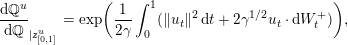 $$\begin{eqnarray}\displaystyle \frac{\text{d}\mathbb{Q}^{u}}{\text{d}\mathbb{Q}}_{|z_{[0,1]}^{u}}=\exp \biggl(\displaystyle \frac{1}{2\unicode[STIX]{x1D6FE}}\int _{0}^{1}(\Vert u_{t}\Vert ^{2}\,\text{d}t+2\unicode[STIX]{x1D6FE}^{1/2}u_{t}\cdot \text{d}W_{t}^{+})\biggr),\end{eqnarray}$$
provided that the Kullback–Leibler divergence
 $\text{KL}(\mathbb{Q}^{u}||\mathbb{Q})$
between
$\text{KL}(\mathbb{Q}^{u}||\mathbb{Q})$
between
 $\mathbb{Q}^{u}$
and
$\mathbb{Q}^{u}$
and
 $\mathbb{Q}$
, given by
$\mathbb{Q}$
, given by
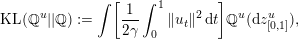 $$\begin{eqnarray}\text{KL}(\mathbb{Q}^{u}||\mathbb{Q}):=\int \biggl[\displaystyle \frac{1}{2\unicode[STIX]{x1D6FE}}\int _{0}^{1}\Vert u_{t}\Vert ^{2}\,\text{d}t\biggr]\mathbb{Q}^{u}(\text{d}z_{[0,1]}^{u}),\end{eqnarray}$$
is finite. Recall that the Kullback–Leibler divergence between two path measures
 $\mathbb{P}\ll \mathbb{Q}$
on
$\mathbb{P}\ll \mathbb{Q}$
on
 ${\mathcal{C}}$
is defined by
${\mathcal{C}}$
is defined by
 $$\begin{eqnarray}\text{KL}(\mathbb{P}||\mathbb{Q})=\int \log \displaystyle \frac{\text{d}\mathbb{P}}{\text{d}\mathbb{Q}}\,\mathbb{P}(\text{d}z_{[0,1]}).\end{eqnarray}$$
If the modified SDE (2.30) is used to make predictions, then its solutions
 $z_{[0,1]}^{u}$
need to be weighted according to the inverse Radon–Nikodym derivative
$z_{[0,1]}^{u}$
need to be weighted according to the inverse Radon–Nikodym derivative
 $$\begin{eqnarray}\displaystyle \frac{\text{d}\mathbb{Q}}{\text{d}\mathbb{Q}^{u}}_{|z_{[0,1]}^{u}}=\exp \biggl(-\displaystyle \frac{1}{2\unicode[STIX]{x1D6FE}}\int _{0}^{1}(\Vert u_{t}\Vert ^{2}\,\text{d}t+2\unicode[STIX]{x1D6FE}^{1/2}u_{t}\cdot \,\text{d}W_{t}^{+})\biggr)\end{eqnarray}$$
in order to reproduce the desired forecast PDF
 $\unicode[STIX]{x1D70B}_{1}$
of the original SDE (2.24).
$\unicode[STIX]{x1D70B}_{1}$
of the original SDE (2.24).
Remark 2.12. A heuristic derivation of equation (2.33) can be found in Section 3.1.2 below, where we discuss the numerical approximation of SDEs by the Euler–Maruyama method. Equation (2.34) follows immediately from (2.33) by noting that the expectation of Brownian motion under the path measure
 $\mathbb{Q}^{u}$
is zero.
$\mathbb{Q}^{u}$
is zero.
2.2 Filtering and smoothing
We now incorporate the likelihood
 $$\begin{eqnarray}l(z_{1})=\unicode[STIX]{x1D70B}(y_{1}|z_{1})\end{eqnarray}$$
of the data
 $y_{1}$
at time
$y_{1}$
at time
 $t_{1}=1$
. Bayes’ theorem tells us that, given the forecast PDF
$t_{1}=1$
. Bayes’ theorem tells us that, given the forecast PDF
 $\unicode[STIX]{x1D70B}_{1}$
at time
$\unicode[STIX]{x1D70B}_{1}$
at time
 $t_{1}$
, the posterior PDF
$t_{1}$
, the posterior PDF
 $\widehat{\unicode[STIX]{x1D70B}}_{1}$
is given by (2.5). The distribution
$\widehat{\unicode[STIX]{x1D70B}}_{1}$
is given by (2.5). The distribution
 $\widehat{\unicode[STIX]{x1D70B}}_{1}$
solves the filtering problem at time
$\widehat{\unicode[STIX]{x1D70B}}_{1}$
solves the filtering problem at time
 $t_{1}$
given the data
$t_{1}$
given the data
 $y_{1}$
. We also recall the definition of the evidence (2.7). The quantity
$y_{1}$
. We also recall the definition of the evidence (2.7). The quantity
 ${\mathcal{F}}=-\log \unicode[STIX]{x1D6FD}$
is called the free energy in statistical physics (Hartmann et al.
Reference Hartmann, Richter, Schütte and Zhang2017).
${\mathcal{F}}=-\log \unicode[STIX]{x1D6FD}$
is called the free energy in statistical physics (Hartmann et al.
Reference Hartmann, Richter, Schütte and Zhang2017).
An appropriate transition kernel
 $q_{1}(\widehat{z}_{1}|z_{1})$
, satisfying (2.11), is required in order to complete the transition from
$q_{1}(\widehat{z}_{1}|z_{1})$
, satisfying (2.11), is required in order to complete the transition from
 $\unicode[STIX]{x1D70B}_{0}$
to
$\unicode[STIX]{x1D70B}_{0}$
to
 $\widehat{\unicode[STIX]{x1D70B}}_{1}$
following scenario (A) from Definition 2.4. A suitable framework for finding such transition kernels is via the theory of optimal transportation (Villani Reference Villani2003). More specifically, let
$\widehat{\unicode[STIX]{x1D70B}}_{1}$
following scenario (A) from Definition 2.4. A suitable framework for finding such transition kernels is via the theory of optimal transportation (Villani Reference Villani2003). More specifically, let
 $\unicode[STIX]{x1D6F1}_{\text{c}}$
denote the set of all joint probability measures
$\unicode[STIX]{x1D6F1}_{\text{c}}$
denote the set of all joint probability measures
 $\unicode[STIX]{x1D70B}(z_{1},\widehat{z}_{1})$
with marginals
$\unicode[STIX]{x1D70B}(z_{1},\widehat{z}_{1})$
with marginals
 $$\begin{eqnarray}\int \unicode[STIX]{x1D70B}(z_{1},\widehat{z}_{1})\,\text{d}\widehat{z}_{1}=\unicode[STIX]{x1D70B}_{1}(z_{1}),\quad \int \unicode[STIX]{x1D70B}(z_{1},\widehat{z}_{1})\,\text{d}z_{1}=\widehat{\unicode[STIX]{x1D70B}}_{1}(\widehat{z}_{1}).\end{eqnarray}$$
We seek the joint measure
 $\unicode[STIX]{x1D70B}^{\ast }(z_{1},\widehat{z}_{1})\in \unicode[STIX]{x1D6F1}_{\text{c}}$
which minimizes the expected Euclidean distance between the two associated random variables
$\unicode[STIX]{x1D70B}^{\ast }(z_{1},\widehat{z}_{1})\in \unicode[STIX]{x1D6F1}_{\text{c}}$
which minimizes the expected Euclidean distance between the two associated random variables
 $Z_{1}$
and
$Z_{1}$
and
 $\widehat{Z}_{1}$
, that is,
$\widehat{Z}_{1}$
, that is,
 $$\begin{eqnarray}\unicode[STIX]{x1D70B}^{\ast }=\arg \inf _{\unicode[STIX]{x1D70B}\in \unicode[STIX]{x1D6F1}_{\text{c}}}\int \int \Vert z_{1}-\widehat{z}_{1}\Vert ^{2}\,\unicode[STIX]{x1D70B}(z_{1},\widehat{z}_{1})\,\text{d}z_{1}\,\text{d}\widehat{z}_{1}.\end{eqnarray}$$
The minimizing joint measure is of the form
 $$\begin{eqnarray}\unicode[STIX]{x1D70B}^{\ast }(z_{1},\widehat{z}_{1})=\unicode[STIX]{x1D6FF}(\widehat{z}_{1}-\unicode[STIX]{x1D6FB}_{z}\unicode[STIX]{x1D6F7}(z_{1}))\,\unicode[STIX]{x1D70B}_{1}(z_{1})\end{eqnarray}$$
with suitable convex potential
 $\unicode[STIX]{x1D6F7}$
under appropriate conditions on the PDFs
$\unicode[STIX]{x1D6F7}$
under appropriate conditions on the PDFs
 $\unicode[STIX]{x1D70B}_{1}$
and
$\unicode[STIX]{x1D70B}_{1}$
and
 $\widehat{\unicode[STIX]{x1D70B}}_{1}$
(Villani Reference Villani2003). These conditions are satisfied for dynamical systems with Gaussian model errors and typical SDE models. Once the potential
$\widehat{\unicode[STIX]{x1D70B}}_{1}$
(Villani Reference Villani2003). These conditions are satisfied for dynamical systems with Gaussian model errors and typical SDE models. Once the potential
 $\unicode[STIX]{x1D6F7}$
(or an approximation) is available, samples
$\unicode[STIX]{x1D6F7}$
(or an approximation) is available, samples
 $z_{1}^{i}$
,
$z_{1}^{i}$
,
 $i=1,\ldots ,M$
, from the forecast PDF
$i=1,\ldots ,M$
, from the forecast PDF
 $\unicode[STIX]{x1D70B}_{1}$
can be converted into samples
$\unicode[STIX]{x1D70B}_{1}$
can be converted into samples
 $\widehat{z}_{1}^{i}$
,
$\widehat{z}_{1}^{i}$
,
 $i=1,\ldots ,M$
, from the filtering distribution
$i=1,\ldots ,M$
, from the filtering distribution
 $\widehat{\unicode[STIX]{x1D70B}}_{1}$
via the deterministic transformation
$\widehat{\unicode[STIX]{x1D70B}}_{1}$
via the deterministic transformation
 $$\begin{eqnarray}\widehat{z}_{1}^{i}=\unicode[STIX]{x1D6FB}_{z}\unicode[STIX]{x1D6F7}(z_{1}^{i}).\end{eqnarray}$$
We will discuss in Section 3 how to approximate the transformation (2.38) numerically. We will find that many popular data assimilation schemes, such as the ensemble Kalman filter, can be viewed as approximations to (2.38) (Reich and Cotter Reference Reich and Cotter2015).
We recall at this point that classical particle filters start from the importance weights
 $$\begin{eqnarray}w^{i}\propto \displaystyle \frac{\widehat{\unicode[STIX]{x1D70B}}_{1}(z_{1}^{i})}{\unicode[STIX]{x1D70B}_{1}(z_{1}^{i})}=\displaystyle \frac{l(z_{1}^{i})}{\unicode[STIX]{x1D6FD}},\end{eqnarray}$$
and obtain the desired samples
 $\widehat{z}^{i}$
by an appropriate resampling with replacement scheme (Doucet et al.
Reference Doucet, de Freitas and Gordon2001, Arulampalam et al.
Reference Arulampalam, Maskell, Gordon and Clapp2002, Douc and Cappe Reference Douc and Cappe2005) instead of applying a deterministic transformation of the form (2.38).
$\widehat{z}^{i}$
by an appropriate resampling with replacement scheme (Doucet et al.
Reference Doucet, de Freitas and Gordon2001, Arulampalam et al.
Reference Arulampalam, Maskell, Gordon and Clapp2002, Douc and Cappe Reference Douc and Cappe2005) instead of applying a deterministic transformation of the form (2.38).
Remark 2.13. If one replaces the forward transition kernel
 $q_{+}(z_{1}|z_{0})$
with a twisted kernel (1.2), then, using (2.17), the filtering distribution (2.5) satisfies
$q_{+}(z_{1}|z_{0})$
with a twisted kernel (1.2), then, using (2.17), the filtering distribution (2.5) satisfies
 $$\begin{eqnarray}\displaystyle \frac{\widehat{\unicode[STIX]{x1D70B}}_{1}(z_{1})}{\unicode[STIX]{x1D70B}_{1}^{\unicode[STIX]{x1D713}}(z_{1})}=\displaystyle \frac{l(z_{1})\mathop{\sum }_{j=1}^{M}q_{+}(z_{1}|z_{0}^{j})}{\unicode[STIX]{x1D6FD}\mathop{\sum }_{j=1}^{M}{\textstyle \frac{\unicode[STIX]{x1D713}(z_{1})}{\widehat{\unicode[STIX]{x1D713}}(z_{0}^{j})}}\,q_{+}(z_{1}|z_{0}^{j})}.\end{eqnarray}$$
Hence drawing samples
 $z_{1}^{i}$
,
$z_{1}^{i}$
,
 $i=1,\ldots ,M$
, from
$i=1,\ldots ,M$
, from
 $\unicode[STIX]{x1D70B}_{1}^{\unicode[STIX]{x1D713}}$
instead of
$\unicode[STIX]{x1D70B}_{1}^{\unicode[STIX]{x1D713}}$
instead of
 $\unicode[STIX]{x1D70B}_{1}$
leads to modified importance weights
$\unicode[STIX]{x1D70B}_{1}$
leads to modified importance weights
 $$\begin{eqnarray}w^{i}\propto \displaystyle \frac{l(z_{1}^{i})\mathop{\sum }_{j=1}^{M}q_{+}(z_{1}^{i}|z_{0}^{j})}{\unicode[STIX]{x1D6FD}\mathop{\sum }_{j=1}^{M}{\textstyle \frac{\unicode[STIX]{x1D713}(z_{1}^{i})}{\widehat{\unicode[STIX]{x1D713}}(z_{0}^{j})}}\,q_{+}(z_{1}^{i}|z_{0}^{j})}.\end{eqnarray}$$
We will demonstrate in Section 2.3 that finding a twisting potential
 $\unicode[STIX]{x1D713}$
such that
$\unicode[STIX]{x1D713}$
such that
 $\widehat{\unicode[STIX]{x1D70B}}_{1}=\unicode[STIX]{x1D70B}_{1}^{\unicode[STIX]{x1D713}}$
, leading to importance weights
$\widehat{\unicode[STIX]{x1D70B}}_{1}=\unicode[STIX]{x1D70B}_{1}^{\unicode[STIX]{x1D713}}$
, leading to importance weights
 $w^{i}=1$
in (2.40), is equivalent to solving the Schrödinger problem (2.58)–(2.61).
$w^{i}=1$
in (2.40), is equivalent to solving the Schrödinger problem (2.58)–(2.61).
The associated smoothing distribution at time
 $t=0$
can be defined as follows. First introduce
$t=0$
can be defined as follows. First introduce
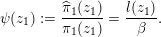 $$\begin{eqnarray}\unicode[STIX]{x1D713}(z_{1}):=\displaystyle \frac{\widehat{\unicode[STIX]{x1D70B}}_{1}(z_{1})}{\unicode[STIX]{x1D70B}_{1}(z_{1})}=\displaystyle \frac{l(z_{1})}{\unicode[STIX]{x1D6FD}}.\end{eqnarray}$$
Next we set
 $$\begin{eqnarray}\widehat{\unicode[STIX]{x1D713}}(z_{0}):=\int q_{+}(z_{1}|z_{0})\,\unicode[STIX]{x1D713}(z_{1})\,\text{d}z_{1}=\unicode[STIX]{x1D6FD}^{-1}\int q_{+}(z_{1}|z_{0})\,l(z_{1})\,\text{d}z_{1},\end{eqnarray}$$
and introduce
 $\widehat{\unicode[STIX]{x1D70B}}_{0}:=\unicode[STIX]{x1D70B}_{0}\,\widehat{\unicode[STIX]{x1D713}}$
, that is,
$\widehat{\unicode[STIX]{x1D70B}}_{0}:=\unicode[STIX]{x1D70B}_{0}\,\widehat{\unicode[STIX]{x1D713}}$
, that is,
 $$\begin{eqnarray}\displaystyle \widehat{\unicode[STIX]{x1D70B}}_{0}(z_{0}) & = & \displaystyle \displaystyle \frac{1}{M}\mathop{\sum }_{i=1}^{M}\widehat{\unicode[STIX]{x1D713}}(z_{0}^{i})\,\unicode[STIX]{x1D6FF}(z_{0}-z_{0}^{i})\nonumber\\ \displaystyle & = & \displaystyle \displaystyle \frac{1}{M}\mathop{\sum }_{i=1}^{M}\unicode[STIX]{x1D6FE}^{i}\,\unicode[STIX]{x1D6FF}(z_{0}-z_{0}^{i})\end{eqnarray}$$
since
 $\widehat{\unicode[STIX]{x1D713}}(z_{0}^{i})=\unicode[STIX]{x1D6FE}^{i}$
with
$\widehat{\unicode[STIX]{x1D713}}(z_{0}^{i})=\unicode[STIX]{x1D6FE}^{i}$
with
 $\unicode[STIX]{x1D6FE}^{i}$
defined by (2.9).
$\unicode[STIX]{x1D6FE}^{i}$
defined by (2.9).
Lemma 2.14. The smoothing PDFs
 $\widehat{\unicode[STIX]{x1D70B}}_{0}$
and
$\widehat{\unicode[STIX]{x1D70B}}_{0}$
and
 $\widehat{\unicode[STIX]{x1D70B}}_{1}$
satisfy
$\widehat{\unicode[STIX]{x1D70B}}_{1}$
satisfy
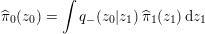 $$\begin{eqnarray}\widehat{\unicode[STIX]{x1D70B}}_{0}(z_{0})=\int q_{-}(z_{0}|z_{1})\,\widehat{\unicode[STIX]{x1D70B}}_{1}(z_{1})\,\text{d}z_{1}\end{eqnarray}$$
with the backward transition kernel defined by (2.15). Furthermore,
 $$\begin{eqnarray}\widehat{\unicode[STIX]{x1D70B}}_{1}(z_{1})=\int \widehat{q}_{+}(z_{1}|z_{0})\,\widehat{\unicode[STIX]{x1D70B}}_{0}(z_{0})\,\text{d}z_{0}\end{eqnarray}$$
with twisted forward transition kernels
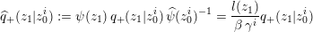 $$\begin{eqnarray}\widehat{q}_{+}(z_{1}|z_{0}^{i}):=\unicode[STIX]{x1D713}(z_{1})\,q_{+}(z_{1}|z_{0}^{i})\,\widehat{\unicode[STIX]{x1D713}}(z_{0}^{i})^{-1}=\displaystyle \frac{l(z_{1})}{\unicode[STIX]{x1D6FD}\,\unicode[STIX]{x1D6FE}^{i}}q_{+}(z_{1}|z_{0}^{i})\end{eqnarray}$$
and
 $\unicode[STIX]{x1D6FE}^{i}$
,
$\unicode[STIX]{x1D6FE}^{i}$
,
 $i=1,\ldots ,M$
, defined by (2.9).
$i=1,\ldots ,M$
, defined by (2.9).
Proof. We note that
 $$\begin{eqnarray}q_{-}(z_{0}|z_{1})\,\widehat{\unicode[STIX]{x1D70B}}_{1}(z_{1})=\displaystyle \frac{\unicode[STIX]{x1D70B}_{0}(z_{0})}{\unicode[STIX]{x1D70B}_{1}(z_{1})}q_{+}(z_{1}|z_{0})\widehat{\unicode[STIX]{x1D70B}}_{1}(z_{1})=\displaystyle \frac{l(z_{1})}{\unicode[STIX]{x1D6FD}}q_{+}(z_{1}|z_{0})\,\unicode[STIX]{x1D70B}_{0}(z_{0}),\end{eqnarray}$$
which implies the first equation. The second equation follows from
 $\widehat{\unicode[STIX]{x1D70B}}_{0}=\widehat{\unicode[STIX]{x1D713}}\,\unicode[STIX]{x1D70B}_{0}$
and
$\widehat{\unicode[STIX]{x1D70B}}_{0}=\widehat{\unicode[STIX]{x1D713}}\,\unicode[STIX]{x1D70B}_{0}$
and
 $$\begin{eqnarray}\int \widehat{q}_{+}(z_{1}|z_{0})\,\widehat{\unicode[STIX]{x1D70B}}_{0}(z_{0})\,\text{d}z_{0}=\displaystyle \frac{1}{M}\mathop{\sum }_{i=1}^{M}\displaystyle \frac{l(z_{1})}{\unicode[STIX]{x1D6FD}}\,q_{+}(z_{1}|z_{0}^{i}).\end{eqnarray}$$
In other words, we have defined a twisted forward transition kernel of the form (1.2).◻
Seen from a more abstract perspective, we have provided an alternative formulation of the joint smoothing distribution
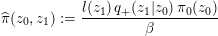 $$\begin{eqnarray}\widehat{\unicode[STIX]{x1D70B}}(z_{0},z_{1}):=\displaystyle \frac{l(z_{1})\,q_{+}(z_{1}|z_{0})\,\unicode[STIX]{x1D70B}_{0}(z_{0})}{\unicode[STIX]{x1D6FD}}\end{eqnarray}$$
in the form of
 $$\begin{eqnarray}\displaystyle \widehat{\unicode[STIX]{x1D70B}}(z_{0},z_{1}) & = & \displaystyle \displaystyle \frac{l(z_{1})}{\unicode[STIX]{x1D6FD}}\displaystyle \frac{\unicode[STIX]{x1D713}(z_{1})}{\unicode[STIX]{x1D713}(z_{1})}q_{+}(z_{1}|z_{0})\displaystyle \frac{\widehat{\unicode[STIX]{x1D713}}(z_{0})}{\widehat{\unicode[STIX]{x1D713}}(z_{0})}\unicode[STIX]{x1D70B}_{0}(z_{0})\nonumber\\ \displaystyle & = & \displaystyle \widehat{q}_{+}(z_{1}|z_{0})\,\widehat{\unicode[STIX]{x1D70B}}_{0}(z_{0})\end{eqnarray}$$
because of (2.41). Note that the marginal distributions of
 $\widehat{\unicode[STIX]{x1D70B}}$
are provided by
$\widehat{\unicode[STIX]{x1D70B}}$
are provided by
 $\widehat{\unicode[STIX]{x1D70B}}_{0}$
and
$\widehat{\unicode[STIX]{x1D70B}}_{0}$
and
 $\widehat{\unicode[STIX]{x1D70B}}_{1}$
, respectively.
$\widehat{\unicode[STIX]{x1D70B}}_{1}$
, respectively.
One can exploit these formulations computationally as follows. If one has generated
 $M$
equally weighted particles
$M$
equally weighted particles
 $\widehat{z}_{0}^{j}$
from the smoothing distribution (2.43) at time
$\widehat{z}_{0}^{j}$
from the smoothing distribution (2.43) at time
 $t=0$
via resampling with replacement, then one can obtain equally weighted samples
$t=0$
via resampling with replacement, then one can obtain equally weighted samples
 $\widehat{z}_{1}^{j}$
from the filtering distribution
$\widehat{z}_{1}^{j}$
from the filtering distribution
 $\widehat{\unicode[STIX]{x1D70B}}_{1}$
using the modified transition kernels (2.45). This is the idea behind the optimal proposal particle filter (Doucet et al.
Reference Doucet, de Freitas and Gordon2001, Arulampalam et al.
Reference Arulampalam, Maskell, Gordon and Clapp2002, Fearnhead and Künsch Reference Fearnhead and Künsch2018) and provides an implementation of scenario (B) as introduced in Definition 2.4.
$\widehat{\unicode[STIX]{x1D70B}}_{1}$
using the modified transition kernels (2.45). This is the idea behind the optimal proposal particle filter (Doucet et al.
Reference Doucet, de Freitas and Gordon2001, Arulampalam et al.
Reference Arulampalam, Maskell, Gordon and Clapp2002, Fearnhead and Künsch Reference Fearnhead and Künsch2018) and provides an implementation of scenario (B) as introduced in Definition 2.4.
Remark 2.15. We remark that backward simulation methods use (2.44) in order to address the smoothing problem (2.2) in a sequential forward–backward manner. Since we are not interested in the general smoothing problem in this paper, we refer the reader to the survey by Lindsten and Schön (Reference Lindsten and Schön2013) for more details.
Lemma 2.16. Let
 $\unicode[STIX]{x1D713}(z)>0$
be a twisting potential such that
$\unicode[STIX]{x1D713}(z)>0$
be a twisting potential such that
 $$\begin{eqnarray}l^{\unicode[STIX]{x1D713}}(z_{1}):=\displaystyle \frac{l(z_{1})}{\unicode[STIX]{x1D6FD}\,\unicode[STIX]{x1D713}(z_{1})}\unicode[STIX]{x1D70B}_{0}[\widehat{\unicode[STIX]{x1D713}}]\end{eqnarray}$$
is well-defined with
 $\widehat{\unicode[STIX]{x1D713}}$
given by (1.3). Then the smoothing PDF (2.46) can be represented as
$\widehat{\unicode[STIX]{x1D713}}$
given by (1.3). Then the smoothing PDF (2.46) can be represented as
 $$\begin{eqnarray}\widehat{\unicode[STIX]{x1D70B}}(z_{0},z_{1})=l^{\unicode[STIX]{x1D713}}(z_{1})\,q_{+}^{\unicode[STIX]{x1D713}}(z_{1}|z_{0})\,\unicode[STIX]{x1D70B}_{0}^{\unicode[STIX]{x1D713}}(z_{0}),\end{eqnarray}$$
where the modified forward transition kernel
 $q_{+}^{\unicode[STIX]{x1D713}}(z_{1}|z_{0})$
is defined by (1.2) and the modified initial PDF by
$q_{+}^{\unicode[STIX]{x1D713}}(z_{1}|z_{0})$
is defined by (1.2) and the modified initial PDF by
 $$\begin{eqnarray}\unicode[STIX]{x1D70B}_{0}^{\unicode[STIX]{x1D713}}(z_{0}):=\displaystyle \frac{\widehat{\unicode[STIX]{x1D713}}(z_{0})\,\unicode[STIX]{x1D70B}_{0}(z_{0})}{\unicode[STIX]{x1D70B}_{0}[\widehat{\unicode[STIX]{x1D713}}]}.\end{eqnarray}$$
Proof. This follows from the definition of the smoothing PDF
 $\widehat{\unicode[STIX]{x1D70B}}(z_{0},z_{1})$
and the twisted transition kernel
$\widehat{\unicode[STIX]{x1D70B}}(z_{0},z_{1})$
and the twisted transition kernel
 $q_{+}^{\unicode[STIX]{x1D713}}(z_{1}|z_{0})$
.◻
$q_{+}^{\unicode[STIX]{x1D713}}(z_{1}|z_{0})$
.◻
Remark 2.17. As mentioned before, the choice (2.41) implies
 $l^{\unicode[STIX]{x1D713}}=\text{const.}$
, and leads to the well-known optimal proposal density for particle filters. The more general formulation (2.48) has recently been explored and expanded by Guarniero et al. (Reference Guarniero, Johansen and Lee2017) and Heng et al. (Reference Heng, Bishop, Deligiannidis and Doucet2018) in order to derive efficient proposal densities for the general smoothing problem (2.2). Within the simplified formulation (2.48), such approaches reduce to a change of measure from
$l^{\unicode[STIX]{x1D713}}=\text{const.}$
, and leads to the well-known optimal proposal density for particle filters. The more general formulation (2.48) has recently been explored and expanded by Guarniero et al. (Reference Guarniero, Johansen and Lee2017) and Heng et al. (Reference Heng, Bishop, Deligiannidis and Doucet2018) in order to derive efficient proposal densities for the general smoothing problem (2.2). Within the simplified formulation (2.48), such approaches reduce to a change of measure from
 $\unicode[STIX]{x1D70B}_{0}$
to
$\unicode[STIX]{x1D70B}_{0}$
to
 $\unicode[STIX]{x1D70B}_{0}^{\unicode[STIX]{x1D713}}$
at
$\unicode[STIX]{x1D70B}_{0}^{\unicode[STIX]{x1D713}}$
at
 $t_{0}$
followed by a forward transition according to
$t_{0}$
followed by a forward transition according to
 $q_{+}^{\unicode[STIX]{x1D713}}$
and subsequent reweighting by a modified likelihood
$q_{+}^{\unicode[STIX]{x1D713}}$
and subsequent reweighting by a modified likelihood
 $l^{\unicode[STIX]{x1D713}}$
at
$l^{\unicode[STIX]{x1D713}}$
at
 $t_{1}$
and hence lead to particle filters that combine scenarios (A) and (B) as introduced in Definition 2.4.
$t_{1}$
and hence lead to particle filters that combine scenarios (A) and (B) as introduced in Definition 2.4.
2.2.1 Gaussian model errors (cont.)
We return to the discrete-time process (2.20) and assume a Gaussian measurement error leading to a Gaussian likelihood
 $$\begin{eqnarray}l(z_{1})\propto \exp \biggl(-\displaystyle \frac{1}{2}(Hz_{1}-y_{1})^{T}R^{-1}(Hz_{1}-y_{1})\biggr).\end{eqnarray}$$
We set
 $\unicode[STIX]{x1D713}_{1}=l/\unicode[STIX]{x1D6FD}$
in order to derive the optimal forward kernel for the associated smoothing/filtering problem. Following the discussion from Section 2.1.1, this leads to the modified transition kernels
$\unicode[STIX]{x1D713}_{1}=l/\unicode[STIX]{x1D6FD}$
in order to derive the optimal forward kernel for the associated smoothing/filtering problem. Following the discussion from Section 2.1.1, this leads to the modified transition kernels
 $$\begin{eqnarray}\widehat{q}_{+}(z_{1}|z_{0}^{i}):=\text{n}(z_{1};\bar{z}_{1}^{i},\unicode[STIX]{x1D6FE}\bar{B})\end{eqnarray}$$
with
 $\bar{B}$
and
$\bar{B}$
and
 $K$
defined by (2.23) and (2.22), respectively, and
$K$
defined by (2.23) and (2.22), respectively, and
 $$\begin{eqnarray}\bar{z}_{1}^{i}:=\unicode[STIX]{x1D6F9}(z_{0}^{i})-K(H\unicode[STIX]{x1D6F9}(z_{0}^{i})-y_{1}).\end{eqnarray}$$
The smoothing distribution
 $\widehat{\unicode[STIX]{x1D70B}}_{0}$
is given by
$\widehat{\unicode[STIX]{x1D70B}}_{0}$
is given by
 $$\begin{eqnarray}\widehat{\unicode[STIX]{x1D70B}}_{0}(z_{0})=\displaystyle \frac{1}{M}\mathop{\sum }_{i=1}^{M}\unicode[STIX]{x1D6FE}^{i}\,\unicode[STIX]{x1D6FF}(z-z_{0}^{i})\end{eqnarray}$$
with coefficients
 $$\begin{eqnarray}\unicode[STIX]{x1D6FE}^{i}\propto \exp \biggl(-\displaystyle \frac{1}{2}(H\unicode[STIX]{x1D6F9}(z_{0}^{i})-y_{1})^{\text{T}}(R+\unicode[STIX]{x1D6FE}HBH^{\text{T}})^{-1}(H\unicode[STIX]{x1D6F9}(z_{0}^{i})-y_{1})\biggr).\end{eqnarray}$$
It is easily checked that, indeed,
 $$\begin{eqnarray}\widehat{\unicode[STIX]{x1D70B}}_{1}(z_{1})=\int q_{+}^{\unicode[STIX]{x1D713}}(z_{1}|z_{0})\,\widehat{\unicode[STIX]{x1D70B}}_{0}(z_{0})\,\text{d}z_{0}.\end{eqnarray}$$
The results from this subsection have been used in simplified form in Example 2.5 in order to compute (2.14). We also note that a non-optimal, i.e.
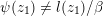 $\unicode[STIX]{x1D713}(z_{1})\not =l(z_{1})/\unicode[STIX]{x1D6FD}$
, but Gaussian choice for
$\unicode[STIX]{x1D713}(z_{1})\not =l(z_{1})/\unicode[STIX]{x1D6FD}$
, but Gaussian choice for
 $\unicode[STIX]{x1D713}$
leads to a Gaussian
$\unicode[STIX]{x1D713}$
leads to a Gaussian
 $l^{\unicode[STIX]{x1D713}}$
and the transition kernels
$l^{\unicode[STIX]{x1D713}}$
and the transition kernels
 $q_{+}^{\unicode[STIX]{x1D713}}(z_{1}|z_{0}^{i})$
in (2.48) remain Gaussian as well. This is in contrast to the Schrödinger problem, which we discuss in the following Section 2.3 and which leads to forward transition kernels of the form (2.66) below.
$q_{+}^{\unicode[STIX]{x1D713}}(z_{1}|z_{0}^{i})$
in (2.48) remain Gaussian as well. This is in contrast to the Schrödinger problem, which we discuss in the following Section 2.3 and which leads to forward transition kernels of the form (2.66) below.
2.2.2 SDE models (cont.)
The likelihood
 $l(z_{1})$
introduces a change of measure over path space
$l(z_{1})$
introduces a change of measure over path space
 $z_{[0,1]}\in {\mathcal{C}}$
from the forecast measure
$z_{[0,1]}\in {\mathcal{C}}$
from the forecast measure
 $\mathbb{Q}$
with marginals
$\mathbb{Q}$
with marginals
 $\unicode[STIX]{x1D70B}_{t}$
to the smoothing measure
$\unicode[STIX]{x1D70B}_{t}$
to the smoothing measure
 $\widehat{\mathbb{P}}$
via the Radon–Nikodym derivative
$\widehat{\mathbb{P}}$
via the Radon–Nikodym derivative
 $$\begin{eqnarray}\displaystyle \frac{\text{d}\widehat{\mathbb{P}}}{\text{d}\mathbb{Q}}_{|z_{[0,1]}}=\displaystyle \frac{l(z_{1})}{\unicode[STIX]{x1D6FD}}.\end{eqnarray}$$
We let
 $\widehat{\unicode[STIX]{x1D70B}}_{t}$
denote the marginal distributions of the smoothing measure
$\widehat{\unicode[STIX]{x1D70B}}_{t}$
denote the marginal distributions of the smoothing measure
 $\widehat{\mathbb{P}}$
at time
$\widehat{\mathbb{P}}$
at time
 $t$
.
$t$
.
Lemma 2.18. Let
 $\unicode[STIX]{x1D713}_{t}$
denote the solution of the backward Kolmogorov equation (2.31) with final condition
$\unicode[STIX]{x1D713}_{t}$
denote the solution of the backward Kolmogorov equation (2.31) with final condition
 $\unicode[STIX]{x1D713}_{1}(z)=l(z)/\unicode[STIX]{x1D6FD}$
at
$\unicode[STIX]{x1D713}_{1}(z)=l(z)/\unicode[STIX]{x1D6FD}$
at
 $t=1$
. Then the controlled forward SDE
$t=1$
. Then the controlled forward SDE
 $$\begin{eqnarray}\text{d}Z_{t}^{+}=(f_{t}(Z_{t}^{+})+\unicode[STIX]{x1D6FE}\unicode[STIX]{x1D6FB}_{z}\log \unicode[STIX]{x1D713}_{t}(Z_{t}^{+}))\,\text{d}t+\unicode[STIX]{x1D6FE}^{1/2}\,\text{d}W_{t}^{+},\end{eqnarray}$$
with
 $Z_{0}^{+}\sim \widehat{\unicode[STIX]{x1D70B}}_{0}$
at time
$Z_{0}^{+}\sim \widehat{\unicode[STIX]{x1D70B}}_{0}$
at time
 $t=0$
, implies
$t=0$
, implies
 $Z_{1}^{+}\sim \widehat{\unicode[STIX]{x1D70B}}_{1}$
at final time
$Z_{1}^{+}\sim \widehat{\unicode[STIX]{x1D70B}}_{1}$
at final time
 $t=1$
.
$t=1$
.
Proof. The lemma is a consequence of Lemma 2.11 and definition (2.45) of the smoothing kernel
 $\widehat{q}_{+}(z_{1}|z_{0})$
with
$\widehat{q}_{+}(z_{1}|z_{0})$
with
 $\unicode[STIX]{x1D713}(z_{1})=\unicode[STIX]{x1D713}_{1}(z_{1})$
and
$\unicode[STIX]{x1D713}(z_{1})=\unicode[STIX]{x1D713}_{1}(z_{1})$
and
 $\widehat{\unicode[STIX]{x1D713}}(z_{0})=\unicode[STIX]{x1D713}_{0}(z_{0})$
.◻
$\widehat{\unicode[STIX]{x1D713}}(z_{0})=\unicode[STIX]{x1D713}_{0}(z_{0})$
.◻
The SDE (2.50) is obviously a special case of (2.30) with control law
 $u_{t}$
given by (2.32). Note, however, that the initial distributions for (2.30) and (2.50) are different. We will reconcile this fact in the following subsection by considering the associated Schrödinger problem (Föllmer and Gantert Reference Föllmer and Gantert1997, Leonard Reference Leonard2014, Chen et al.
Reference Chen, Georgiou and Pavon2014).
$u_{t}$
given by (2.32). Note, however, that the initial distributions for (2.30) and (2.50) are different. We will reconcile this fact in the following subsection by considering the associated Schrödinger problem (Föllmer and Gantert Reference Föllmer and Gantert1997, Leonard Reference Leonard2014, Chen et al.
Reference Chen, Georgiou and Pavon2014).
Lemma 2.19. The solution
 $\unicode[STIX]{x1D713}_{t}$
of the backward Kolmogorov equation (2.31) with final condition
$\unicode[STIX]{x1D713}_{t}$
of the backward Kolmogorov equation (2.31) with final condition
 $\unicode[STIX]{x1D713}_{1}(z)=l(z)/\unicode[STIX]{x1D6FD}$
at
$\unicode[STIX]{x1D713}_{1}(z)=l(z)/\unicode[STIX]{x1D6FD}$
at
 $t=1$
satisfies
$t=1$
satisfies
 $$\begin{eqnarray}\unicode[STIX]{x1D713}_{t}(z)=\displaystyle \frac{\widehat{\unicode[STIX]{x1D70B}}_{t}(z)}{\unicode[STIX]{x1D70B}_{t}(z)}\end{eqnarray}$$
and the PDFs
 $\widehat{\unicode[STIX]{x1D70B}}_{t}$
coincide with the marginal PDFs of the backward SDE (2.28) with final condition
$\widehat{\unicode[STIX]{x1D70B}}_{t}$
coincide with the marginal PDFs of the backward SDE (2.28) with final condition
 $Z_{1}^{-}\sim \widehat{\unicode[STIX]{x1D70B}}_{1}$
.
$Z_{1}^{-}\sim \widehat{\unicode[STIX]{x1D70B}}_{1}$
.
Proof. We first note that (2.51) holds at final time
 $t=1$
. Furthermore, equation (2.51) implies
$t=1$
. Furthermore, equation (2.51) implies
 $$\begin{eqnarray}\unicode[STIX]{x2202}_{t}\widehat{\unicode[STIX]{x1D70B}}_{t}=\unicode[STIX]{x1D70B}_{t}\,\unicode[STIX]{x2202}_{t}\unicode[STIX]{x1D713}_{t}-\unicode[STIX]{x1D713}_{t}\,\unicode[STIX]{x2202}_{t}\unicode[STIX]{x1D70B}_{t}.\end{eqnarray}$$
Since
 $\unicode[STIX]{x1D70B}_{t}$
satisfies the Fokker–Planck equation (2.26) and
$\unicode[STIX]{x1D70B}_{t}$
satisfies the Fokker–Planck equation (2.26) and
 $\unicode[STIX]{x1D713}_{t}$
the backward Kolmogorov equation (2.31), it follows that
$\unicode[STIX]{x1D713}_{t}$
the backward Kolmogorov equation (2.31), it follows that
 $$\begin{eqnarray}\unicode[STIX]{x2202}_{t}\widehat{\unicode[STIX]{x1D70B}}_{t}=-\unicode[STIX]{x1D6FB}_{z}\cdot (\widehat{\unicode[STIX]{x1D70B}}_{t}(f-\unicode[STIX]{x1D6FE}\unicode[STIX]{x1D6FB}_{z}\log \unicode[STIX]{x1D70B}_{t}))-\displaystyle \frac{\unicode[STIX]{x1D6FE}}{2}\unicode[STIX]{x1D6E5}_{z}\widehat{\unicode[STIX]{x1D70B}}_{t},\end{eqnarray}$$
which corresponds to the Fokker–Planck equation (2.27) of the backward SDE (2.28) with final condition
 $Z_{1}^{-}\sim \widehat{\unicode[STIX]{x1D70B}}_{1}$
and marginal PDFs denoted by
$Z_{1}^{-}\sim \widehat{\unicode[STIX]{x1D70B}}_{1}$
and marginal PDFs denoted by
 $\widehat{\unicode[STIX]{x1D70B}}_{t}$
instead of
$\widehat{\unicode[STIX]{x1D70B}}_{t}$
instead of
 $\unicode[STIX]{x1D70B}_{t}$
.◻
$\unicode[STIX]{x1D70B}_{t}$
.◻
Note that (2.52) is equivalent to
 $$\begin{eqnarray}\unicode[STIX]{x2202}\widehat{\unicode[STIX]{x1D70B}}_{t}=-\unicode[STIX]{x1D6FB}_{z}\cdot (\widehat{\unicode[STIX]{x1D70B}}_{t}(f-\unicode[STIX]{x1D6FE}\unicode[STIX]{x1D6FB}_{z}\log \unicode[STIX]{x1D70B}_{t}+\unicode[STIX]{x1D6FE}\unicode[STIX]{x1D6FB}_{z}\log \widehat{\unicode[STIX]{x1D70B}}_{t}))+\displaystyle \frac{\unicode[STIX]{x1D6FE}}{2}\unicode[STIX]{x1D6E5}_{z}\widehat{\unicode[STIX]{x1D70B}}_{t},\end{eqnarray}$$
which in turn is equivalent to the Fokker–Planck equation of the forward smoothing SDE (2.50) since
 $\unicode[STIX]{x1D713}_{t}=\widehat{\unicode[STIX]{x1D70B}}_{t}/\unicode[STIX]{x1D70B}_{t}$
.
$\unicode[STIX]{x1D713}_{t}=\widehat{\unicode[STIX]{x1D70B}}_{t}/\unicode[STIX]{x1D70B}_{t}$
.
We conclude from the previous lemma that one can either solve the backward Kolmogorov equation (2.31) with
 $\unicode[STIX]{x1D713}_{1}(z)=l(z)/\unicode[STIX]{x1D6FD}$
or the backward SDE (2.28) with
$\unicode[STIX]{x1D713}_{1}(z)=l(z)/\unicode[STIX]{x1D6FD}$
or the backward SDE (2.28) with
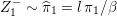 $Z_{1}^{-}\sim \widehat{\unicode[STIX]{x1D70B}}_{1}=l\,\unicode[STIX]{x1D70B}_{1}/\unicode[STIX]{x1D6FD}$
in order to derive the desired control law
$Z_{1}^{-}\sim \widehat{\unicode[STIX]{x1D70B}}_{1}=l\,\unicode[STIX]{x1D70B}_{1}/\unicode[STIX]{x1D6FD}$
in order to derive the desired control law
 $u_{t}(z)=\unicode[STIX]{x1D6FE}\unicode[STIX]{x1D6FB}_{z}\log \unicode[STIX]{x1D713}_{t}$
in (2.50).
$u_{t}(z)=\unicode[STIX]{x1D6FE}\unicode[STIX]{x1D6FB}_{z}\log \unicode[STIX]{x1D713}_{t}$
in (2.50).
Remark 2.20. The notion of a backward SDE used throughout this paper is different from the notion of a backward SDE in the sense of Carmona (Reference Carmona2016), for example. More specifically, Itô’s formula
 $$\begin{eqnarray}\text{d}\unicode[STIX]{x1D713}_{t}=\unicode[STIX]{x2202}_{t}\unicode[STIX]{x1D713}_{t}\,\,\text{d}t+\unicode[STIX]{x1D6FB}_{z}\unicode[STIX]{x1D713}_{t}\cdot \,\text{d}Z_{t}^{+}+\displaystyle \frac{\unicode[STIX]{x1D6FE}}{2}\unicode[STIX]{x1D6E5}_{z}\unicode[STIX]{x1D713}_{t}\,\text{d}t\end{eqnarray}$$
and the fact that
 $\unicode[STIX]{x1D713}_{t}$
satisfies the backward Kolmogorov equation (2.31) imply that
$\unicode[STIX]{x1D713}_{t}$
satisfies the backward Kolmogorov equation (2.31) imply that
 $$\begin{eqnarray}\text{d}\unicode[STIX]{x1D713}_{t}=\unicode[STIX]{x1D6FE}^{1/2}\,\unicode[STIX]{x1D6FB}_{z}\unicode[STIX]{x1D713}_{t}\cdot \,\text{d}W_{t}^{+}\end{eqnarray}$$
along solutions of the forward SDE (2.24). In other words, the quantities
 $\unicode[STIX]{x1D713}_{t}$
are materially advected along solutions
$\unicode[STIX]{x1D713}_{t}$
are materially advected along solutions
 $Z_{t}^{+}$
of the forward SDEs in expectation or, in the language of stochastic analysis,
$Z_{t}^{+}$
of the forward SDEs in expectation or, in the language of stochastic analysis,
 $\unicode[STIX]{x1D713}_{t}$
is a martingale. Hence, by the martingale representation theorem, we can reformulate the problem of determining
$\unicode[STIX]{x1D713}_{t}$
is a martingale. Hence, by the martingale representation theorem, we can reformulate the problem of determining
 $\unicode[STIX]{x1D713}_{t}$
as follows. Find the solution
$\unicode[STIX]{x1D713}_{t}$
as follows. Find the solution
 $(Y_{t},V_{t})$
of the backward SDE
$(Y_{t},V_{t})$
of the backward SDE
 $$\begin{eqnarray}\text{d}Y_{t}=V_{t}\cdot \,\text{d}W_{t}^{+}\end{eqnarray}$$
subject to the final condition
 $Y_{1}=l(Z_{1}^{+})/\unicode[STIX]{x1D6FD}$
at
$Y_{1}=l(Z_{1}^{+})/\unicode[STIX]{x1D6FD}$
at
 $t=1$
. Here (2.54) has to be understood as a backward SDE in the sense of Carmona (Reference Carmona2016), for example, where the solution
$t=1$
. Here (2.54) has to be understood as a backward SDE in the sense of Carmona (Reference Carmona2016), for example, where the solution
 $(Y_{t},V_{t})$
is adapted to the forward SDE (2.24), i.e. to the past
$(Y_{t},V_{t})$
is adapted to the forward SDE (2.24), i.e. to the past
 $s\leq t$
, whereas the solution
$s\leq t$
, whereas the solution
 $Z_{t}^{-}$
of the backward SDE (2.28) is adapted to the future
$Z_{t}^{-}$
of the backward SDE (2.28) is adapted to the future
 $s\geq t$
. The solution of (2.54) is given by
$s\geq t$
. The solution of (2.54) is given by
 $Y_{t}=\unicode[STIX]{x1D713}_{t}(Z_{t}^{+})$
and
$Y_{t}=\unicode[STIX]{x1D713}_{t}(Z_{t}^{+})$
and
 $V_{t}=\unicode[STIX]{x1D6FE}^{1/2}\,\unicode[STIX]{x1D6FB}_{z}\unicode[STIX]{x1D713}_{t}(Z_{t}^{+})$
in agreement with (2.53) (compare Carmona Reference Carmona2016, page 42). See Appendix A.4 for the numerical treatment of (2.54).
$V_{t}=\unicode[STIX]{x1D6FE}^{1/2}\,\unicode[STIX]{x1D6FB}_{z}\unicode[STIX]{x1D713}_{t}(Z_{t}^{+})$
in agreement with (2.53) (compare Carmona Reference Carmona2016, page 42). See Appendix A.4 for the numerical treatment of (2.54).
A variational characterization of the smoothing path measure
 $\widehat{\mathbb{P}}$
is given by the Donsker–Varadhan principle
$\widehat{\mathbb{P}}$
is given by the Donsker–Varadhan principle
 $$\begin{eqnarray}\widehat{\mathbb{P}}=\arg \inf _{\mathbb{P}\ll \mathbb{Q}}\{-\mathbb{P}[\log (l)]+\text{KL}(\mathbb{P}||\mathbb{Q})\},\end{eqnarray}$$
that is, the distribution
 $\widehat{\mathbb{P}}$
is chosen such that the expected loss,
$\widehat{\mathbb{P}}$
is chosen such that the expected loss,
 $-\mathbb{P}[\log (l)]$
, is minimized subject to the penalty introduced by the Kullback–Leibler divergence with respect to the original path measure
$-\mathbb{P}[\log (l)]$
, is minimized subject to the penalty introduced by the Kullback–Leibler divergence with respect to the original path measure
 $\mathbb{Q}$
. Note that
$\mathbb{Q}$
. Note that
 $$\begin{eqnarray}\inf _{\mathbb{P}\ll \mathbb{Q}}\{\mathbb{P}[-\log (l)]+\text{KL}(\mathbb{P}||\mathbb{Q})\}=-\log \unicode[STIX]{x1D6FD}\end{eqnarray}$$
with
 $\unicode[STIX]{x1D6FD}=\mathbb{Q}[l]$
. The connection between smoothing for SDEs and the Donsker–Varadhan principle has, for example, been discussed by Mitter and Newton (Reference Mitter and Newton2003). See also Hartmann et al. (Reference Hartmann, Richter, Schütte and Zhang2017) for an in-depth discussion of variational formulations and their numerical implementation in the context of rare event simulations for which it is generally assumed that
$\unicode[STIX]{x1D6FD}=\mathbb{Q}[l]$
. The connection between smoothing for SDEs and the Donsker–Varadhan principle has, for example, been discussed by Mitter and Newton (Reference Mitter and Newton2003). See also Hartmann et al. (Reference Hartmann, Richter, Schütte and Zhang2017) for an in-depth discussion of variational formulations and their numerical implementation in the context of rare event simulations for which it is generally assumed that
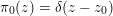 $\unicode[STIX]{x1D70B}_{0}(z)=\unicode[STIX]{x1D6FF}(z-z_{0})$
in (2.3), that is, the ensemble size is
$\unicode[STIX]{x1D70B}_{0}(z)=\unicode[STIX]{x1D6FF}(z-z_{0})$
in (2.3), that is, the ensemble size is
 $M=1$
when viewed within the context of this paper.
$M=1$
when viewed within the context of this paper.
Remark 2.21. One can choose
 $\unicode[STIX]{x1D713}_{t}$
differently from the choice made in (2.51) by changing the final condition for the backward Kolmogorov equation (2.31) to any suitable
$\unicode[STIX]{x1D713}_{t}$
differently from the choice made in (2.51) by changing the final condition for the backward Kolmogorov equation (2.31) to any suitable
 $\unicode[STIX]{x1D713}_{1}$
. As already discussed for twisted discrete-time smoothing, such modifications give rise to alternative representations of the smoothing distribution
$\unicode[STIX]{x1D713}_{1}$
. As already discussed for twisted discrete-time smoothing, such modifications give rise to alternative representations of the smoothing distribution
 $\widehat{\mathbb{P}}$
in terms of modified forward SDEs, likelihood functions and initial distributions. See Kappen and Ruiz (Reference Kappen and Ruiz2016) and Ruiz and Kappen (Reference Ruiz and Kappen2017) for an application of these ideas to importance sampling in the context of partially observed diffusion processes. More specifically, let
$\widehat{\mathbb{P}}$
in terms of modified forward SDEs, likelihood functions and initial distributions. See Kappen and Ruiz (Reference Kappen and Ruiz2016) and Ruiz and Kappen (Reference Ruiz and Kappen2017) for an application of these ideas to importance sampling in the context of partially observed diffusion processes. More specifically, let
 $u_{t}$
denote the associated control law (2.32) for the forward SDE (2.30) with given initial distribution
$u_{t}$
denote the associated control law (2.32) for the forward SDE (2.30) with given initial distribution
 $Z_{0}^{+}\sim q_{0}$
. Then
$Z_{0}^{+}\sim q_{0}$
. Then
 $$\begin{eqnarray}\displaystyle \frac{\text{d}\widehat{\mathbb{P}}}{\text{d}\mathbb{Q}}_{|z_{[0,1]}^{u}}=\displaystyle \frac{\text{d}\widehat{\mathbb{P}}}{\text{d}\mathbb{Q}^{u}}_{|z_{[0,1]}^{u}}\,\displaystyle \frac{\text{d}\mathbb{Q}^{u}}{\text{d}\mathbb{Q}}_{|z_{[0,1]}^{u}},\end{eqnarray}$$
which, using (2.33) and (2.49), implies the modified Radon–Nikodym derivative
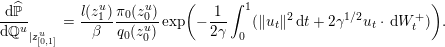 $$\begin{eqnarray}\displaystyle \frac{\text{d}\widehat{\mathbb{P}}}{\text{d}\mathbb{Q}^{u}}_{|z_{[0,1]}^{u}}=\displaystyle \frac{l(z_{1}^{u})}{\unicode[STIX]{x1D6FD}}\displaystyle \frac{\unicode[STIX]{x1D70B}_{0}(z_{0}^{u})}{q_{0}(z_{0}^{u})}\exp \biggl(-\displaystyle \frac{1}{2\unicode[STIX]{x1D6FE}}\int _{0}^{1}(\Vert u_{t}\Vert ^{2}\,\text{d}t+2\unicode[STIX]{x1D6FE}^{1/2}u_{t}\cdot \,\text{d}W_{t}^{+})\biggr).\end{eqnarray}$$
Recall from Lemma 2.18 that the control law (2.32) with
 $\unicode[STIX]{x1D713}_{t}$
defined by (2.51) together with
$\unicode[STIX]{x1D713}_{t}$
defined by (2.51) together with
 $q_{0}=\widehat{\unicode[STIX]{x1D70B}}_{0}$
leads to
$q_{0}=\widehat{\unicode[STIX]{x1D70B}}_{0}$
leads to
 $\widehat{\mathbb{P}}=\mathbb{Q}^{u}$
.
$\widehat{\mathbb{P}}=\mathbb{Q}^{u}$
.
2.3 Schrödinger problem
In this subsection we show that scenario (C) from Definition 2.4 leads to a certain boundary value problem first considered by Schrödinger (Reference Schrödinger1931). More specifically, we state the so-called Schrödinger problem and show how it is linked to data assimilation scenario (C).
In order to introduce the Schrödinger problem, we return to the twisting potential approach as utilized in Section 2.2, with two important modifications. These modifications are, first, that the twisting potential
 $\unicode[STIX]{x1D713}$
is determined implicitly and, second, that the modified transition kernel
$\unicode[STIX]{x1D713}$
is determined implicitly and, second, that the modified transition kernel
 $q_{+}^{\unicode[STIX]{x1D713}}$
is applied to
$q_{+}^{\unicode[STIX]{x1D713}}$
is applied to
 $\unicode[STIX]{x1D70B}_{0}$
instead of the tilted initial density
$\unicode[STIX]{x1D70B}_{0}$
instead of the tilted initial density
 $\unicode[STIX]{x1D70B}_{0}^{\unicode[STIX]{x1D713}}$
as in (2.48). More specifically, we have the following.
$\unicode[STIX]{x1D70B}_{0}^{\unicode[STIX]{x1D713}}$
as in (2.48). More specifically, we have the following.
Definition 2.22. We seek the pair of functions
 $\widehat{\unicode[STIX]{x1D713}}(z_{0})$
and
$\widehat{\unicode[STIX]{x1D713}}(z_{0})$
and
 $\unicode[STIX]{x1D713}(z_{1})$
which solve the boundary value problem
$\unicode[STIX]{x1D713}(z_{1})$
which solve the boundary value problem
 $$\begin{eqnarray}\displaystyle \unicode[STIX]{x1D70B}_{0}(z_{0}) & = & \displaystyle \unicode[STIX]{x1D70B}_{0}^{\unicode[STIX]{x1D713}}(z_{0})\,\widehat{\unicode[STIX]{x1D713}}(z_{0}),\end{eqnarray}$$
 $$\begin{eqnarray}\displaystyle \widehat{\unicode[STIX]{x1D70B}}_{1}(z_{1}) & = & \displaystyle \unicode[STIX]{x1D70B}_{1}^{\unicode[STIX]{x1D713}}(z_{1})\,\unicode[STIX]{x1D713}(z_{1}),\end{eqnarray}$$
 $$\begin{eqnarray}\displaystyle \unicode[STIX]{x1D70B}_{1}^{\unicode[STIX]{x1D713}}(z_{1}) & = & \displaystyle \int q_{+}(z_{1}|z_{0})\,\unicode[STIX]{x1D70B}_{0}^{\unicode[STIX]{x1D713}}(z_{0})\,\text{d}z_{0},\end{eqnarray}$$
 $$\begin{eqnarray}\displaystyle \widehat{\unicode[STIX]{x1D713}}(z_{0}) & = & \displaystyle \int q_{+}(z_{1}|z_{0})\,\unicode[STIX]{x1D713}(z_{1})\,\text{d}z_{1},\end{eqnarray}$$
for given marginal (filtering) distributions
 $\unicode[STIX]{x1D70B}_{0}$
and
$\unicode[STIX]{x1D70B}_{0}$
and
 $\widehat{\unicode[STIX]{x1D70B}}_{1}$
at
$\widehat{\unicode[STIX]{x1D70B}}_{1}$
at
 $t=0$
and
$t=0$
and
 $t=1$
, respectively. The required modified PDFs
$t=1$
, respectively. The required modified PDFs
 $\unicode[STIX]{x1D70B}_{0}^{\unicode[STIX]{x1D713}}$
and
$\unicode[STIX]{x1D70B}_{0}^{\unicode[STIX]{x1D713}}$
and
 $\unicode[STIX]{x1D70B}_{1}^{\unicode[STIX]{x1D713}}$
are defined by (2.58) and (2.59), respectively. The solution
$\unicode[STIX]{x1D70B}_{1}^{\unicode[STIX]{x1D713}}$
are defined by (2.58) and (2.59), respectively. The solution
 $(\widehat{\unicode[STIX]{x1D713}},\unicode[STIX]{x1D713})$
of the Schrödinger system (2.58)–(2.61) leads to the modified transition kernel
$(\widehat{\unicode[STIX]{x1D713}},\unicode[STIX]{x1D713})$
of the Schrödinger system (2.58)–(2.61) leads to the modified transition kernel
 $$\begin{eqnarray}q_{+}^{\ast }(z_{1}|z_{0}):=\unicode[STIX]{x1D713}(z_{1})\,q_{+}(z_{1}|z_{0})\,\widehat{\unicode[STIX]{x1D713}}(z_{0})^{-1},\end{eqnarray}$$
which satisfies
 $$\begin{eqnarray}\widehat{\unicode[STIX]{x1D70B}}_{1}(z_{1})=\int q_{+}^{\ast }(z_{1}|z_{0})\,\unicode[STIX]{x1D70B}_{0}(z_{0})\,\text{d}z_{0}\end{eqnarray}$$
by construction.
The modified transition kernel
 $q_{+}^{\ast }(z_{1}|z_{0})$
couples the two marginal distributions
$q_{+}^{\ast }(z_{1}|z_{0})$
couples the two marginal distributions
 $\unicode[STIX]{x1D70B}_{0}$
and
$\unicode[STIX]{x1D70B}_{0}$
and
 $\widehat{\unicode[STIX]{x1D70B}}_{1}$
with the twisting potential
$\widehat{\unicode[STIX]{x1D70B}}_{1}$
with the twisting potential
 $\unicode[STIX]{x1D713}$
implicitly defined. In other words,
$\unicode[STIX]{x1D713}$
implicitly defined. In other words,
 $q_{+}^{\ast }$
provides the transition kernel for going from the initial distribution (2.3) at time
$q_{+}^{\ast }$
provides the transition kernel for going from the initial distribution (2.3) at time
 $t_{0}$
to the filtering distribution at time
$t_{0}$
to the filtering distribution at time
 $t_{1}$
without the need for any reweighting, i.e. the desired transition kernel for scenario (C). See Leonard (Reference Leonard2014) and Chen et al. (Reference Chen, Georgiou and Pavon2014) for more mathematical details on the Schrödinger problem.
$t_{1}$
without the need for any reweighting, i.e. the desired transition kernel for scenario (C). See Leonard (Reference Leonard2014) and Chen et al. (Reference Chen, Georgiou and Pavon2014) for more mathematical details on the Schrödinger problem.
Remark 2.23. Let us compare the Schrödinger system to the twisting potential approach (2.48) for the smoothing problem from Section 2.2 in some more detail. First, note that the twisting potential approach to smoothing replaces (2.58) with
 $$\begin{eqnarray}\unicode[STIX]{x1D70B}_{0}^{\unicode[STIX]{x1D713}}(z_{0})=\unicode[STIX]{x1D70B}_{0}(z_{0})\,\widehat{\unicode[STIX]{x1D713}}(z_{0})\end{eqnarray}$$
and (2.59) with
 $$\begin{eqnarray}\unicode[STIX]{x1D70B}_{1}^{\unicode[STIX]{x1D713}}(z_{1})=\unicode[STIX]{x1D70B}_{1}(z_{1})\,\unicode[STIX]{x1D713}(z_{1}),\end{eqnarray}$$
where
 $\unicode[STIX]{x1D713}$
is a given twisting potential normalized such that
$\unicode[STIX]{x1D713}$
is a given twisting potential normalized such that
 $\unicode[STIX]{x1D70B}_{1}[\unicode[STIX]{x1D713}]=1$
. The associated
$\unicode[STIX]{x1D70B}_{1}[\unicode[STIX]{x1D713}]=1$
. The associated
 $\widehat{\unicode[STIX]{x1D713}}$
is determined by (2.61) as in the twisting approach. In both cases, the modified transition kernel is given by (2.62). Finally, (2.60) is replaced by the prediction step (2.4).
$\widehat{\unicode[STIX]{x1D713}}$
is determined by (2.61) as in the twisting approach. In both cases, the modified transition kernel is given by (2.62). Finally, (2.60) is replaced by the prediction step (2.4).
In order to solve the Schrödinger system for our given initial distribution (2.3) and the associated filter distribution
 $\widehat{\unicode[STIX]{x1D70B}}_{1}$
, we make the ansatz
$\widehat{\unicode[STIX]{x1D70B}}_{1}$
, we make the ansatz
 $$\begin{eqnarray}\unicode[STIX]{x1D70B}_{0}^{\unicode[STIX]{x1D713}}(z_{0})=\displaystyle \frac{1}{M}\mathop{\sum }_{i=1}^{M}\unicode[STIX]{x1D6FC}^{i}\,\unicode[STIX]{x1D6FF}(z_{0}-z_{0}^{i}),\quad \mathop{\sum }_{i=1}^{M}\unicode[STIX]{x1D6FC}^{i}=M.\end{eqnarray}$$
This ansatz together with (2.58)–(2.61) immediately implies
 $$\begin{eqnarray}\widehat{\unicode[STIX]{x1D713}}(z_{0}^{i})=\displaystyle \frac{1}{\unicode[STIX]{x1D6FC}^{i}},\quad \unicode[STIX]{x1D70B}_{1}^{\unicode[STIX]{x1D713}}(z_{1})=\displaystyle \frac{1}{M}\mathop{\sum }_{i=1}^{M}\unicode[STIX]{x1D6FC}^{i}\,q_{+}(z_{1}|z_{0}^{i}),\end{eqnarray}$$
as well as
 $$\begin{eqnarray}\unicode[STIX]{x1D713}(z_{1})=\displaystyle \frac{\widehat{\unicode[STIX]{x1D70B}}_{1}(z_{1})}{\unicode[STIX]{x1D70B}_{1}^{\unicode[STIX]{x1D713}}(z_{1})}=\displaystyle \frac{l(z_{1})}{\unicode[STIX]{x1D6FD}}\displaystyle \frac{{\textstyle \frac{1}{M}}\mathop{\sum }_{j=1}^{M}q_{+}(z_{1}|z_{0}^{j})}{{\textstyle \frac{1}{M}}\mathop{\sum }_{j=1}^{M}\unicode[STIX]{x1D6FC}^{j}\,q_{+}(z_{1}|z_{0}^{j})}.\end{eqnarray}$$
Hence we arrive at the equations
 $$\begin{eqnarray}\displaystyle \widehat{\unicode[STIX]{x1D713}}(z_{0}^{i}) & = & \displaystyle \displaystyle \frac{1}{\unicode[STIX]{x1D6FC}^{i}}\end{eqnarray}$$
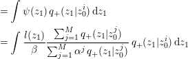 $$\begin{eqnarray}\displaystyle & = & \displaystyle \int \unicode[STIX]{x1D713}(z_{1})\,q_{+}(z_{1}|z_{0}^{i})\,\text{d}z_{1}\nonumber\\ \displaystyle & = & \displaystyle \int \displaystyle \frac{l(z_{1})}{\unicode[STIX]{x1D6FD}}\displaystyle \frac{\mathop{\sum }_{j=1}^{M}q_{+}(z_{1}|z_{0}^{j})}{\mathop{\sum }_{j=1}^{M}\unicode[STIX]{x1D6FC}^{j}\,q_{+}(z_{1}|z_{0}^{j})}\,q_{+}(z_{1}|z_{0}^{i})\,\text{d}z_{1}\end{eqnarray}$$
for
 $i=1,\ldots ,M$
. These
$i=1,\ldots ,M$
. These
 $M$
equations have to be solved for the
$M$
equations have to be solved for the
 $M$
unknown coefficients
$M$
unknown coefficients
 $\{\unicode[STIX]{x1D6FC}^{i}\}$
. In other words, the Schrödinger problem becomes finite-dimensional in the context of this paper. More specifically, we have the following result.
$\{\unicode[STIX]{x1D6FC}^{i}\}$
. In other words, the Schrödinger problem becomes finite-dimensional in the context of this paper. More specifically, we have the following result.
Lemma 2.24. The forward Schrödinger transition kernel (2.62) is given by
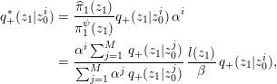 $$\begin{eqnarray}\displaystyle q_{+}^{\ast }(z_{1}|z_{0}^{i}) & = & \displaystyle \displaystyle \frac{\widehat{\unicode[STIX]{x1D70B}}_{1}(z_{1})}{\unicode[STIX]{x1D70B}_{1}^{\unicode[STIX]{x1D713}}(z_{1})}q_{+}(z_{1}|z_{0}^{i})\,\unicode[STIX]{x1D6FC}^{i}\nonumber\\ \displaystyle & = & \displaystyle \displaystyle \frac{\unicode[STIX]{x1D6FC}^{i}\mathop{\sum }_{j=1}^{M}\,q_{+}(z_{1}|z_{0}^{j})}{\mathop{\sum }_{j=1}^{M}\unicode[STIX]{x1D6FC}^{j}\,q_{+}(z_{1}|z_{0}^{j})}\,\displaystyle \frac{l(z_{1})}{\unicode[STIX]{x1D6FD}}\,q_{+}(z_{1}|z_{0}^{i}),\end{eqnarray}$$
for each particle
 $z_{0}^{i}$
with the coefficients
$z_{0}^{i}$
with the coefficients
 $\unicode[STIX]{x1D6FC}^{j}$
,
$\unicode[STIX]{x1D6FC}^{j}$
,
 $j=1,\ldots ,M$
, defined by (2.64)–(2.65).
$j=1,\ldots ,M$
, defined by (2.64)–(2.65).
Proof. Because of (2.64)–(2.65), the forward transition kernels (2.66) satisfy
 $$\begin{eqnarray}\int q_{+}^{\ast }(z_{1}|z_{0}^{i})\,\text{d}z_{1}=1\end{eqnarray}$$
for all
 $i=1,\ldots ,M$
and
$i=1,\ldots ,M$
and
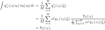 $$\begin{eqnarray}\displaystyle \int q_{+}^{\ast }(z_{1}|z_{0})\,\unicode[STIX]{x1D70B}_{0}(z_{0})\,\text{d}z & = & \displaystyle \displaystyle \frac{1}{M}\mathop{\sum }_{i=1}^{M}q_{+}^{\ast }(z_{1}|z_{0}^{i})\nonumber\\ \displaystyle & = & \displaystyle \displaystyle \frac{1}{M}\mathop{\sum }_{i=1}^{M}\unicode[STIX]{x1D6FC}^{i}q_{+}(z_{1}|z_{0}^{i})\,\displaystyle \frac{\widehat{\unicode[STIX]{x1D70B}}_{1}(z_{1})}{{\textstyle \frac{1}{M}}\mathop{\sum }_{j=1}^{M}\unicode[STIX]{x1D6FC}^{j}\,q_{+}(z_{1}|z_{0}^{j})}\nonumber\\ \displaystyle & = & \displaystyle \widehat{\unicode[STIX]{x1D70B}}_{1}(z_{1}),\end{eqnarray}$$
as desired. ◻
Numerical implementations will be discussed in Section 3. Note that knowledge of the normalizing constant
 $\unicode[STIX]{x1D6FD}$
is not required a priori for solving (2.64)–(2.65) since it appears as a common scaling factor.
$\unicode[STIX]{x1D6FD}$
is not required a priori for solving (2.64)–(2.65) since it appears as a common scaling factor.
We note that the coefficients
 $\{\unicode[STIX]{x1D6FC}^{j}\}$
together with the associated potential
$\{\unicode[STIX]{x1D6FC}^{j}\}$
together with the associated potential
 $\unicode[STIX]{x1D713}$
from the Schrödinger system provide the optimally twisted prediction kernel (1.2) with respect to the filtering distribution
$\unicode[STIX]{x1D713}$
from the Schrödinger system provide the optimally twisted prediction kernel (1.2) with respect to the filtering distribution
 $\widehat{\unicode[STIX]{x1D70B}}_{1}$
, that is, we set
$\widehat{\unicode[STIX]{x1D70B}}_{1}$
, that is, we set
 $\widehat{\unicode[STIX]{x1D713}}(z_{0}^{i})=1/\unicode[STIX]{x1D6FC}^{i}$
in (2.16) and define the potential
$\widehat{\unicode[STIX]{x1D713}}(z_{0}^{i})=1/\unicode[STIX]{x1D6FC}^{i}$
in (2.16) and define the potential
 $\unicode[STIX]{x1D713}$
by (2.63).
$\unicode[STIX]{x1D713}$
by (2.63).
Lemma 2.25. The Schrödinger transition kernel (2.62) satisfies the following constrained variational principle. Consider the joint PDFs given by
 $\unicode[STIX]{x1D70B}(z_{0},z_{1}):=q_{+}(z_{1}|z_{0})\unicode[STIX]{x1D70B}_{0}(z_{0})$
and
$\unicode[STIX]{x1D70B}(z_{0},z_{1}):=q_{+}(z_{1}|z_{0})\unicode[STIX]{x1D70B}_{0}(z_{0})$
and
 $\unicode[STIX]{x1D70B}^{\ast }(z_{0},z_{1}):=q_{+}^{\ast }(z_{1}|z_{0})\unicode[STIX]{x1D70B}_{0}(z_{0})$
. Then
$\unicode[STIX]{x1D70B}^{\ast }(z_{0},z_{1}):=q_{+}^{\ast }(z_{1}|z_{0})\unicode[STIX]{x1D70B}_{0}(z_{0})$
. Then
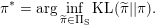 $$\begin{eqnarray}\unicode[STIX]{x1D70B}^{\ast }=\arg \inf _{\widetilde{\unicode[STIX]{x1D70B}}\in \unicode[STIX]{x1D6F1}_{\text{S}}}\text{KL}(\widetilde{\unicode[STIX]{x1D70B}}||\unicode[STIX]{x1D70B}).\end{eqnarray}$$
Here a joint PDF
 $\widetilde{\unicode[STIX]{x1D70B}}(z_{0},z_{1})$
is an element of
$\widetilde{\unicode[STIX]{x1D70B}}(z_{0},z_{1})$
is an element of
 $\unicode[STIX]{x1D6F1}_{\text{S}}$
if
$\unicode[STIX]{x1D6F1}_{\text{S}}$
if
 $$\begin{eqnarray}\int \widetilde{\unicode[STIX]{x1D70B}}(z_{0},z_{1})\,\text{d}z_{1}=\unicode[STIX]{x1D70B}_{0}(z_{0}),\quad \int \widetilde{\unicode[STIX]{x1D70B}}(z_{0},z_{1})\,\text{d}z_{0}=\widehat{\unicode[STIX]{x1D70B}}_{1}(z_{1}).\end{eqnarray}$$
Proof. See Föllmer and Gantert (Reference Föllmer and Gantert1997) for a proof and Remark 2.31 for a heuristic derivation in the case of discrete measures.◻
The constrained variational formulation (2.69) of Schrödinger’s problem should be compared to the unconstrained Donsker–Varadhan variational principle
 $$\begin{eqnarray}\widehat{\unicode[STIX]{x1D70B}}=\arg \inf \{-\widetilde{\unicode[STIX]{x1D70B}}[\log (l)]+\text{KL}(\widetilde{\unicode[STIX]{x1D70B}}||\unicode[STIX]{x1D70B})\}\end{eqnarray}$$
for the associated smoothing problem. See Remark 2.27 below.
Remark 2.26. The Schrödinger problem is closely linked to optimal transportation (Cuturi Reference Cuturi and Burges2013, Leonard Reference Leonard2014, Chen et al.
Reference Chen, Georgiou and Pavon2014). For example, consider the Gaussian transition kernel (2.21) with
 $\unicode[STIX]{x1D6F9}(z)=z$
and
$\unicode[STIX]{x1D6F9}(z)=z$
and
 $B=I$
. Then the solution (2.66) to the associated Schrödinger problem of coupling
$B=I$
. Then the solution (2.66) to the associated Schrödinger problem of coupling
 $\unicode[STIX]{x1D70B}_{0}$
and
$\unicode[STIX]{x1D70B}_{0}$
and
 $\widehat{\unicode[STIX]{x1D70B}}_{1}$
reduces to the solution
$\widehat{\unicode[STIX]{x1D70B}}_{1}$
reduces to the solution
 $\unicode[STIX]{x1D70B}^{\ast }$
of the associated optimal transport problem
$\unicode[STIX]{x1D70B}^{\ast }$
of the associated optimal transport problem
 $$\begin{eqnarray}\unicode[STIX]{x1D70B}^{\ast }=\arg \inf _{\widetilde{\unicode[STIX]{x1D70B}}\in \unicode[STIX]{x1D6F1}_{\text{S}}}\int \int \Vert z_{0}-z_{1}\Vert ^{2}\,\widetilde{\unicode[STIX]{x1D70B}}(z_{0},z_{1})\,\text{d}z_{0}\,\text{d}z_{1}\end{eqnarray}$$
in the limit
 $\unicode[STIX]{x1D6FE}\rightarrow 0$
.
$\unicode[STIX]{x1D6FE}\rightarrow 0$
.
2.3.1 SDE models (cont.)
At the SDE level, Schrödinger’s problem amounts to continuously bridging the given initial PDF
 $\unicode[STIX]{x1D70B}_{0}$
with the PDF
$\unicode[STIX]{x1D70B}_{0}$
with the PDF
 $\widehat{\unicode[STIX]{x1D70B}}_{1}$
at final time using an appropriate modification of the stochastic process
$\widehat{\unicode[STIX]{x1D70B}}_{1}$
at final time using an appropriate modification of the stochastic process
 $Z_{[0,1]}^{+}\sim \mathbb{Q}$
defined by the forward SDE (2.24) with initial distribution
$Z_{[0,1]}^{+}\sim \mathbb{Q}$
defined by the forward SDE (2.24) with initial distribution
 $\unicode[STIX]{x1D70B}_{0}$
at
$\unicode[STIX]{x1D70B}_{0}$
at
 $t=0$
. The desired modified stochastic process
$t=0$
. The desired modified stochastic process
 $\mathbb{P}^{\ast }$
is defined as the minimizer of
$\mathbb{P}^{\ast }$
is defined as the minimizer of
 $$\begin{eqnarray}{\mathcal{L}}(\widetilde{\mathbb{P}}):=\text{KL}(\widetilde{\mathbb{P}}||\mathbb{Q})\end{eqnarray}$$
subject to the constraint that the marginal distributions
 $\widetilde{\unicode[STIX]{x1D70B}}_{t}$
of
$\widetilde{\unicode[STIX]{x1D70B}}_{t}$
of
 $\widetilde{\mathbb{P}}$
at time
$\widetilde{\mathbb{P}}$
at time
 $t=0$
and
$t=0$
and
 $t=1$
satisfy
$t=1$
satisfy
 $\unicode[STIX]{x1D70B}_{0}$
and
$\unicode[STIX]{x1D70B}_{0}$
and
 $\widehat{\unicode[STIX]{x1D70B}}_{1}$
, respectively (Föllmer and Gantert Reference Föllmer and Gantert1997, Leonard Reference Leonard2014, Chen et al.
Reference Chen, Georgiou and Pavon2014).
$\widehat{\unicode[STIX]{x1D70B}}_{1}$
, respectively (Föllmer and Gantert Reference Föllmer and Gantert1997, Leonard Reference Leonard2014, Chen et al.
Reference Chen, Georgiou and Pavon2014).
Remark 2.27. We note that the Donsker–Varadhan variational principle (2.55), characterizing the smoothing path measure
 $\widehat{\mathbb{P}}$
, can be replaced by
$\widehat{\mathbb{P}}$
, can be replaced by
 $$\begin{eqnarray}\mathbb{P}^{\ast }=\arg \inf _{\widetilde{\mathbb{ P}}\in \unicode[STIX]{x1D6F1}}\{-\widetilde{\unicode[STIX]{x1D70B}}_{1}[\log (l)]+\text{KL}(\widetilde{\mathbb{P}}||\mathbb{Q})\}\end{eqnarray}$$
with
 $$\begin{eqnarray}\unicode[STIX]{x1D6F1}=\{\widetilde{\mathbb{P}}\ll \mathbb{Q}:\,\widetilde{\unicode[STIX]{x1D70B}}_{1}=\widehat{\unicode[STIX]{x1D70B}}_{1},\,\widetilde{\unicode[STIX]{x1D70B}}_{0}=\unicode[STIX]{x1D70B}_{0}\}\end{eqnarray}$$
in the context of Schrödinger’s problem. The associated
 $$\begin{eqnarray}-\log \unicode[STIX]{x1D6FD}^{\ast }:=\inf _{\widetilde{\mathbb{ P}}\in \unicode[STIX]{x1D6F1}}\{-\widetilde{\unicode[STIX]{x1D70B}}_{1}[\log (l)]+\text{KL}(\widetilde{\mathbb{P}}||\mathbb{Q})\}=-\widehat{\unicode[STIX]{x1D70B}}[\log (l)]+\text{KL}(\mathbb{P}^{\ast }||\mathbb{Q})\end{eqnarray}$$
can be viewed as a generalization of (2.56) and gives rise to a generalized evidence
 $\unicode[STIX]{x1D6FD}^{\ast }$
, which could be used for model comparison and parameter estimation.
$\unicode[STIX]{x1D6FD}^{\ast }$
, which could be used for model comparison and parameter estimation.
The Schrödinger process
 $\mathbb{P}^{\ast }$
corresponds to a Markovian process across the whole time domain
$\mathbb{P}^{\ast }$
corresponds to a Markovian process across the whole time domain
 $[0,1]$
(Leonard Reference Leonard2014, Chen et al.
Reference Chen, Georgiou and Pavon2014). More specifically, consider the controlled forward SDE (2.30) with initial conditions
$[0,1]$
(Leonard Reference Leonard2014, Chen et al.
Reference Chen, Georgiou and Pavon2014). More specifically, consider the controlled forward SDE (2.30) with initial conditions
 $$\begin{eqnarray}Z_{0}^{+}\sim \unicode[STIX]{x1D70B}_{0}\end{eqnarray}$$
and a given control law
 $u_{t}$
for
$u_{t}$
for
 $t\in [0,1]$
. Let
$t\in [0,1]$
. Let
 $\mathbb{P}^{u}$
denote the path measure associated to this process. Then, as discussed in detail by Dai Pra (Reference Dai Pra1991), one can find time-dependent potentials
$\mathbb{P}^{u}$
denote the path measure associated to this process. Then, as discussed in detail by Dai Pra (Reference Dai Pra1991), one can find time-dependent potentials
 $\unicode[STIX]{x1D713}_{t}$
with associated control laws (2.32) such that the marginal of the associated path measure
$\unicode[STIX]{x1D713}_{t}$
with associated control laws (2.32) such that the marginal of the associated path measure
 $\mathbb{P}^{u}$
at times
$\mathbb{P}^{u}$
at times
 $t=1$
satisfies
$t=1$
satisfies
 $$\begin{eqnarray}\unicode[STIX]{x1D70B}_{1}^{u}=\widehat{\unicode[STIX]{x1D70B}}_{1}\end{eqnarray}$$
and, more generally,
 $$\begin{eqnarray}\mathbb{P}^{\ast }=\mathbb{P}^{u}.\end{eqnarray}$$
We summarize this result in the following lemma.
Lemma 2.28. The Schrödinger path measure
 $\mathbb{P}^{\ast }$
can be generated by a controlled SDE (2.30) with control law (2.32), where the desired potential
$\mathbb{P}^{\ast }$
can be generated by a controlled SDE (2.30) with control law (2.32), where the desired potential
 $\unicode[STIX]{x1D713}_{t}$
can be obtained as follows. Let
$\unicode[STIX]{x1D713}_{t}$
can be obtained as follows. Let
 $(\widehat{\unicode[STIX]{x1D713}},\unicode[STIX]{x1D713})$
denote the solution of the associated Schrödinger system (2.58)–(2.61), where
$(\widehat{\unicode[STIX]{x1D713}},\unicode[STIX]{x1D713})$
denote the solution of the associated Schrödinger system (2.58)–(2.61), where
 $q_{+}(z_{1}|z_{0})$
denotes the time-one forward transition kernel of (2.24). Then
$q_{+}(z_{1}|z_{0})$
denotes the time-one forward transition kernel of (2.24). Then
 $\unicode[STIX]{x1D713}_{t}$
in (2.32) is the solution of the backward Kolmogorov equation (2.31) with prescribed
$\unicode[STIX]{x1D713}_{t}$
in (2.32) is the solution of the backward Kolmogorov equation (2.31) with prescribed
 $\unicode[STIX]{x1D713}_{1}=\unicode[STIX]{x1D713}$
at final time
$\unicode[STIX]{x1D713}_{1}=\unicode[STIX]{x1D713}$
at final time
 $t=1$
.
$t=1$
.
Remark 2.29. As already pointed out in the context of smoothing, the desired potential
 $\unicode[STIX]{x1D713}_{t}$
can also be obtained by solving an appropriate backward SDE. More specifically, given the solution
$\unicode[STIX]{x1D713}_{t}$
can also be obtained by solving an appropriate backward SDE. More specifically, given the solution
 $(\widehat{\unicode[STIX]{x1D713}},\unicode[STIX]{x1D713})$
and the implied PDF
$(\widehat{\unicode[STIX]{x1D713}},\unicode[STIX]{x1D713})$
and the implied PDF
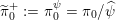 $\widetilde{\unicode[STIX]{x1D70B}}_{0}^{+}:=\unicode[STIX]{x1D70B}_{0}^{\unicode[STIX]{x1D713}}=\unicode[STIX]{x1D70B}_{0}/\widehat{\unicode[STIX]{x1D713}}$
of the Schrödinger system (2.58)–(2.61), let
$\widetilde{\unicode[STIX]{x1D70B}}_{0}^{+}:=\unicode[STIX]{x1D70B}_{0}^{\unicode[STIX]{x1D713}}=\unicode[STIX]{x1D70B}_{0}/\widehat{\unicode[STIX]{x1D713}}$
of the Schrödinger system (2.58)–(2.61), let
 $\widetilde{\unicode[STIX]{x1D70B}}_{t}^{+}$
,
$\widetilde{\unicode[STIX]{x1D70B}}_{t}^{+}$
,
 $t\geq 0$
, denote the marginals of the forward SDE (2.24) with
$t\geq 0$
, denote the marginals of the forward SDE (2.24) with
 $Z_{0}^{+}\sim \widetilde{\unicode[STIX]{x1D70B}}_{0}^{+}$
. Furthermore, consider the backward SDE (2.28) with drift term
$Z_{0}^{+}\sim \widetilde{\unicode[STIX]{x1D70B}}_{0}^{+}$
. Furthermore, consider the backward SDE (2.28) with drift term
 $$\begin{eqnarray}b_{t}(z)=f_{t}(z)-\unicode[STIX]{x1D6FE}\unicode[STIX]{x1D6FB}_{z}\log \widetilde{\unicode[STIX]{x1D70B}}_{t}^{+}(z),\end{eqnarray}$$
and final time condition
 $Z_{1}^{-}\sim \widehat{\unicode[STIX]{x1D70B}}_{1}$
. Then the choice of
$Z_{1}^{-}\sim \widehat{\unicode[STIX]{x1D70B}}_{1}$
. Then the choice of
 $\widetilde{\unicode[STIX]{x1D70B}}_{0}^{+}$
ensures that
$\widetilde{\unicode[STIX]{x1D70B}}_{0}^{+}$
ensures that
 $Z_{0}^{-}\sim \unicode[STIX]{x1D70B}_{0}$
. Furthermore the desired control in (2.30) is provided by
$Z_{0}^{-}\sim \unicode[STIX]{x1D70B}_{0}$
. Furthermore the desired control in (2.30) is provided by
 $$\begin{eqnarray}u_{t}=\unicode[STIX]{x1D6FE}\unicode[STIX]{x1D6FB}_{z}\log \displaystyle \frac{\widetilde{\unicode[STIX]{x1D70B}}_{t}^{-}}{\widetilde{\unicode[STIX]{x1D70B}}_{t}^{+}},\end{eqnarray}$$
where
 $\widetilde{\unicode[STIX]{x1D70B}}_{t}^{-}$
denotes the marginal distributions of the backward SDE (2.28) with drift term (2.71) and
$\widetilde{\unicode[STIX]{x1D70B}}_{t}^{-}$
denotes the marginal distributions of the backward SDE (2.28) with drift term (2.71) and
 $\widetilde{\unicode[STIX]{x1D70B}}_{1}^{-}=\widehat{\unicode[STIX]{x1D70B}}_{1}$
. We will return to this reformulation of the Schrödinger problem in Section 3 when considering it as the limit of a sequence of smoothing problems.
$\widetilde{\unicode[STIX]{x1D70B}}_{1}^{-}=\widehat{\unicode[STIX]{x1D70B}}_{1}$
. We will return to this reformulation of the Schrödinger problem in Section 3 when considering it as the limit of a sequence of smoothing problems.
Remark 2.30. The solution to the Schrödinger problem for linear SDEs and Gaussian marginal distributions has been discussed in detail by Chen, Georgiou and Pavon (Reference Chen, Georgiou and Pavon2016b ).
2.3.2 Discrete measures
We finally discuss the Schrödinger problem in the context of finite-state Markov chains in more detail. These results will be needed in the following sections on the numerical implementation of the Schrödinger approach to sequential data assimilation.
Let us therefore consider an example which will be closely related to the discussion in Section 3. We are given a bi-stochastic matrix
 $Q\in \mathbb{R}^{L\times M}$
with all entries satisfying
$Q\in \mathbb{R}^{L\times M}$
with all entries satisfying
 $q_{lj}>0$
and two discrete probability measures represented by vectors
$q_{lj}>0$
and two discrete probability measures represented by vectors
 $p_{1}\in \mathbb{R}^{L}$
and
$p_{1}\in \mathbb{R}^{L}$
and
 $p_{0}\in \mathbb{R}^{M}$
, respectively. Again we assume for simplicity that all entries in
$p_{0}\in \mathbb{R}^{M}$
, respectively. Again we assume for simplicity that all entries in
 $p_{1}$
and
$p_{1}$
and
 $p_{0}$
are strictly positive. We introduce the set of all bi-stochastic
$p_{0}$
are strictly positive. We introduce the set of all bi-stochastic
 $L\times M$
matrices with those discrete probability measures as marginals, that is,
$L\times M$
matrices with those discrete probability measures as marginals, that is,
 $$\begin{eqnarray}\unicode[STIX]{x1D6F1}_{\text{s}}:=\{P\in \mathbb{R}^{L\times M}:\,P\geq 0,\,P^{\text{T}}\unicode[STIX]{x1D7D9}_{L}=p_{0},\,P\unicode[STIX]{x1D7D9}_{M}=p_{1}\}.\end{eqnarray}$$
Solving Schrödinger’s system (2.58)–(2.61) corresponds to finding two non-negative vectors
 $u\in \mathbb{R}^{L}$
and
$u\in \mathbb{R}^{L}$
and
 $v\in \mathbb{R}^{M}$
such that
$v\in \mathbb{R}^{M}$
such that
 $$\begin{eqnarray}P^{\ast }:=D(u)\,Q\,D(v)^{-1}\in \unicode[STIX]{x1D6F1}_{\text{s}}.\end{eqnarray}$$
In turns out that
 $P^{\ast }$
is uniquely determined and minimizes the Kullback–Leibler divergence between all
$P^{\ast }$
is uniquely determined and minimizes the Kullback–Leibler divergence between all
 $P\in \unicode[STIX]{x1D6F1}_{\text{s}}$
and the reference matrix
$P\in \unicode[STIX]{x1D6F1}_{\text{s}}$
and the reference matrix
 $Q$
, that is,
$Q$
, that is,
 $$\begin{eqnarray}P^{\ast }=\arg \min _{P\in \unicode[STIX]{x1D6F1}_{\text{s}}}\text{KL}\,(P||Q).\end{eqnarray}$$
See Peyre and Cuturi (Reference Peyre and Cuturi2018) and the following remark for more details.
Remark 2.31. If one makes the ansatz
 $$\begin{eqnarray}p_{lj}=\displaystyle \frac{u_{l}q_{lj}}{v_{j}},\end{eqnarray}$$
then the minimization problem (2.73) becomes equivalent to
 $$\begin{eqnarray}P^{\ast }=\arg \min _{(u,v)>0}\mathop{\sum }_{l,j}p_{lj}(\log u_{l}-\log v_{j})\end{eqnarray}$$
subject to the additional constraints
 $$\begin{eqnarray}P\,\unicode[STIX]{x1D7D9}_{M}=D(u)QD(v)^{-1}\,\unicode[STIX]{x1D7D9}_{M}=p_{1},\,P^{\text{T}}\,\unicode[STIX]{x1D7D9}_{L}=D(v)^{-1}Q^{\text{T}}D(u)\,\unicode[STIX]{x1D7D9}_{L}=p_{0}.\end{eqnarray}$$
Note that these constraint determine
 $u>0$
and
$u>0$
and
 $v>0$
up to a common scaling factor. Hence (2.73) can be reduced to finding
$v>0$
up to a common scaling factor. Hence (2.73) can be reduced to finding
 $(u,v)>0$
such that
$(u,v)>0$
such that
 $$\begin{eqnarray}u^{\text{T}}\unicode[STIX]{x1D7D9}_{L}=1,\quad P\unicode[STIX]{x1D7D9}_{M}=p_{1},\quad P^{\text{T}}\unicode[STIX]{x1D7D9}_{L}=p_{0}.\end{eqnarray}$$
Hence we have shown that solving the Schrödinger system is equivalent to solving the minimization problem (2.73) for discrete measures. Thus
 $$\begin{eqnarray}\min _{P\in \unicode[STIX]{x1D6F1}_{\text{s}}}\text{KL}\,(P||Q)=p_{1}^{\text{T}}\log u-p_{0}^{\text{T}}\log v.\end{eqnarray}$$
Lemma 2.32. The Sinkhorn iteration (Sinkhorn Reference Sinkhorn1967)
 $$\begin{eqnarray}\displaystyle u^{k+1} & := & \displaystyle D(P^{2k}\unicode[STIX]{x1D7D9}_{M})^{-1}\,p_{1},\end{eqnarray}$$
 $$\begin{eqnarray}\displaystyle P^{2k+1} & := & \displaystyle D(u^{k+1})\,P^{2k},\end{eqnarray}$$
 $$\begin{eqnarray}\displaystyle v^{k+1} & := & \displaystyle D(p_{0})^{-1}\,(P^{2k+1})^{\text{T}}\,\unicode[STIX]{x1D7D9}_{L},\end{eqnarray}$$
 $$\begin{eqnarray}\displaystyle P^{2k+2} & := & \displaystyle P^{2k+1}\,D(v^{k+1})^{-1},\end{eqnarray}$$
 $k=0,1,\ldots ,$
with initial
$k=0,1,\ldots ,$
with initial
 $P^{0}=Q\in \mathbb{R}^{L\times M}$
provides an algorithm for computing
$P^{0}=Q\in \mathbb{R}^{L\times M}$
provides an algorithm for computing
 $P^{\ast }$
, that is,
$P^{\ast }$
, that is,
 $$\begin{eqnarray}\lim _{k\rightarrow \infty }P^{k}=P^{\ast }.\end{eqnarray}$$
Proof. See, for example, Peyre and Cuturi (Reference Peyre and Cuturi2018) for a proof of (2.78), which is based on the contraction property of the iteration (2.74)–(2.77) with respect to the Hilbert metric on the projective cone of positive vectors.◻
It follows from (2.78) that
 $$\begin{eqnarray}\lim _{k\rightarrow \infty }u^{k}=\unicode[STIX]{x1D7D9}_{L},\quad \lim _{k\rightarrow \infty }v^{k}=\unicode[STIX]{x1D7D9}_{M}.\end{eqnarray}$$
The essential idea of the Sinkhorn iteration is to enforce
 $$\begin{eqnarray}P^{2k+1}\,\unicode[STIX]{x1D7D9}_{M}=p_{1},\quad (P^{2k})^{\text{T}}\,\unicode[STIX]{x1D7D9}_{L}=p_{0}\end{eqnarray}$$
at each iteration step and that the matrix
 $P^{\ast }$
satisfies both constraints simultaneously in the limit
$P^{\ast }$
satisfies both constraints simultaneously in the limit
 $k\rightarrow \infty$
. See Cuturi (Reference Cuturi and Burges2013) for a computationally efficient and robust implementation of the Sinkhorn iteration.
$k\rightarrow \infty$
. See Cuturi (Reference Cuturi and Burges2013) for a computationally efficient and robust implementation of the Sinkhorn iteration.
Remark 2.33. One can introduce a similar iteration for the Schrödinger system (2.58)–(2.61). For example, pick
 $\widehat{\unicode[STIX]{x1D713}}(z_{0})=1$
initially. Then (2.58) implies
$\widehat{\unicode[STIX]{x1D713}}(z_{0})=1$
initially. Then (2.58) implies
 $\unicode[STIX]{x1D70B}_{0}^{\unicode[STIX]{x1D713}}=\unicode[STIX]{x1D70B}_{0}$
and (2.60)
$\unicode[STIX]{x1D70B}_{0}^{\unicode[STIX]{x1D713}}=\unicode[STIX]{x1D70B}_{0}$
and (2.60)
 $\unicode[STIX]{x1D70B}_{1}^{\unicode[STIX]{x1D713}}=\unicode[STIX]{x1D70B}_{1}$
. Hence
$\unicode[STIX]{x1D70B}_{1}^{\unicode[STIX]{x1D713}}=\unicode[STIX]{x1D70B}_{1}$
. Hence
 $\unicode[STIX]{x1D713}=l/\unicode[STIX]{x1D6FD}$
in the first iteration. The second iteration starts with
$\unicode[STIX]{x1D713}=l/\unicode[STIX]{x1D6FD}$
in the first iteration. The second iteration starts with
 $\widehat{\unicode[STIX]{x1D713}}$
determined by (2.61) with
$\widehat{\unicode[STIX]{x1D713}}$
determined by (2.61) with
 $\unicode[STIX]{x1D713}=l/\unicode[STIX]{x1D6FD}$
. We again cycle through (2.58), (2.60) and (2.59) in order to find the next approximation to
$\unicode[STIX]{x1D713}=l/\unicode[STIX]{x1D6FD}$
. We again cycle through (2.58), (2.60) and (2.59) in order to find the next approximation to
 $\unicode[STIX]{x1D713}$
. The third iteration takes now this
$\unicode[STIX]{x1D713}$
. The third iteration takes now this
 $\unicode[STIX]{x1D713}$
and computes the associated
$\unicode[STIX]{x1D713}$
and computes the associated
 $\widehat{\unicode[STIX]{x1D713}}$
from (2.61) etc. A numerical implementation of this procedure requires the approximation of two integrals which essentially leads back to a Sinkhorn type algorithm in the weights of an appropriate quadrature rule.
$\widehat{\unicode[STIX]{x1D713}}$
from (2.61) etc. A numerical implementation of this procedure requires the approximation of two integrals which essentially leads back to a Sinkhorn type algorithm in the weights of an appropriate quadrature rule.
3 Numerical methods
Having summarized the relevant mathematical foundation for prediction, filtering (data assimilation scenario (A)) and smoothing (scenario (B)) and the Schrödinger problem (scenario (C)), we now discuss numerical approximations suitable for ensemble-based data assimilation. It is clearly impossible to cover all available methods, and we will focus on a selection of approaches which are built around the idea of optimal transport, ensemble transform methods and Schrödinger systems. We will also focus on methods that can be applied or extended to problems with high-dimensional state spaces even though we will not explicitly cover this topic in this survey. See Reich and Cotter (Reference Reich and Cotter2015), van Leeuwen (Reference van Leeuwen and van Leeuwen2015) and Asch et al. (Reference Asch, Bocquet and Nodet2017) instead.
3.1 Prediction
Generating samples from the forecast distributions
 $q_{+}(\cdot \,|z_{0}^{i})$
is in most cases straightforward. The computational expenses can, however, vary dramatically, and this impacts on the choice of algorithms for sequential data assimilation. We demonstrate in this subsection how samples from the prediction PDF
$q_{+}(\cdot \,|z_{0}^{i})$
is in most cases straightforward. The computational expenses can, however, vary dramatically, and this impacts on the choice of algorithms for sequential data assimilation. We demonstrate in this subsection how samples from the prediction PDF
 $\unicode[STIX]{x1D70B}_{1}$
can be used to construct an associated finite-state Markov chain that transforms
$\unicode[STIX]{x1D70B}_{1}$
can be used to construct an associated finite-state Markov chain that transforms
 $\unicode[STIX]{x1D70B}_{0}$
into an empirical approximation of
$\unicode[STIX]{x1D70B}_{0}$
into an empirical approximation of
 $\unicode[STIX]{x1D70B}_{1}$
.
$\unicode[STIX]{x1D70B}_{1}$
.
Definition 3.1. Let us assume that we have
 $L\geq M$
independent samples
$L\geq M$
independent samples
 $z_{1}^{l}$
from the
$z_{1}^{l}$
from the
 $M$
forecast distributions
$M$
forecast distributions
 $q_{+}(\cdot \,|z_{0}^{j})$
,
$q_{+}(\cdot \,|z_{0}^{j})$
,
 $j=1,\ldots ,M$
. We introduce the
$j=1,\ldots ,M$
. We introduce the
 $L\times M$
matrix
$L\times M$
matrix
 $Q$
with entries
$Q$
with entries
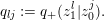 $$\begin{eqnarray}q_{lj}:=q_{+}(z_{1}^{l}|z_{0}^{j}).\end{eqnarray}$$
We now consider the associated bi-stochastic matrix
 $P^{\ast }\in \mathbb{R}^{L\times M}$
, as defined by (2.73), with the two probability vectors in (2.72) given by
$P^{\ast }\in \mathbb{R}^{L\times M}$
, as defined by (2.73), with the two probability vectors in (2.72) given by
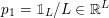 $p_{1}=\unicode[STIX]{x1D7D9}_{L}/L\in \mathbb{R}^{L}$
and
$p_{1}=\unicode[STIX]{x1D7D9}_{L}/L\in \mathbb{R}^{L}$
and
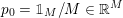 $p_{0}=\unicode[STIX]{x1D7D9}_{M}/M\in \mathbb{R}^{M}$
, respectively. The finite-state Markov chain
$p_{0}=\unicode[STIX]{x1D7D9}_{M}/M\in \mathbb{R}^{M}$
, respectively. The finite-state Markov chain
 $$\begin{eqnarray}Q_{+}:=MP^{\ast }\end{eqnarray}$$
provides a sample-based approximation to the forward transition kernel
 $q_{+}(z_{1}|z_{0})$
.
$q_{+}(z_{1}|z_{0})$
.
More precisely, the
 $i$
th column of
$i$
th column of
 $Q_{+}$
provides an empirical approximation to
$Q_{+}$
provides an empirical approximation to
 $q_{+}(\cdot |z_{0}^{i})$
and
$q_{+}(\cdot |z_{0}^{i})$
and
 $$\begin{eqnarray}Q_{+}\,p_{0}=p_{1}=\displaystyle \frac{1}{L}\unicode[STIX]{x1D7D9}_{L},\end{eqnarray}$$
which is in agreement with the fact that the
 $z_{1}^{l}$
are equally weighted samples from the forecast PDF
$z_{1}^{l}$
are equally weighted samples from the forecast PDF
 $\unicode[STIX]{x1D70B}_{1}$
.
$\unicode[STIX]{x1D70B}_{1}$
.
Remark 3.2. Because of the simple relation between a bi-stochastic matrix
 $P\in \unicode[STIX]{x1D6F1}_{\text{s}}$
with
$P\in \unicode[STIX]{x1D6F1}_{\text{s}}$
with
 $p_{0}$
in (2.72) given by
$p_{0}$
in (2.72) given by
 $p_{0}=\unicode[STIX]{x1D7D9}_{M}/M$
and its associated finite-state Markov chain
$p_{0}=\unicode[STIX]{x1D7D9}_{M}/M$
and its associated finite-state Markov chain
 $Q_{+}=MP$
, one can reformulate the minimization problem (2.73) in those cases directly in terms of Markov chains
$Q_{+}=MP$
, one can reformulate the minimization problem (2.73) in those cases directly in terms of Markov chains
 $Q_{+}\in \unicode[STIX]{x1D6F1}_{\text{M}}$
with the definition of
$Q_{+}\in \unicode[STIX]{x1D6F1}_{\text{M}}$
with the definition of
 $\unicode[STIX]{x1D6F1}_{\text{s}}$
adjusted to
$\unicode[STIX]{x1D6F1}_{\text{s}}$
adjusted to
 $$\begin{eqnarray}\unicode[STIX]{x1D6F1}_{\text{M}}:=\bigg\{Q\in \mathbb{R}^{L\times M}:\,Q\geq 0,\,Q^{\text{T}}\unicode[STIX]{x1D7D9}_{L}=\unicode[STIX]{x1D7D9}_{M},\,\displaystyle \frac{1}{M}Q\unicode[STIX]{x1D7D9}_{M}=p_{1}\bigg\}.\end{eqnarray}$$
Remark 3.3. The associated backward transition kernel
 $Q_{-}\in \mathbb{R}^{M\times L}$
satisfies
$Q_{-}\in \mathbb{R}^{M\times L}$
satisfies
 $$\begin{eqnarray}Q_{-}\,D(p_{1})=(Q_{+}\,D(p_{0}))^{\text{T}}\end{eqnarray}$$
and is hence given by
 $$\begin{eqnarray}Q_{-}=(Q_{+}\,D(p_{0}))^{\text{T}}\,D(p_{1})^{-1}=\displaystyle \frac{L}{M}Q_{+}^{\text{T}}.\end{eqnarray}$$
Thus
 $$\begin{eqnarray}Q_{-}\,p_{1}=D(p_{0})\,Q_{+}^{\text{T}}\,\unicode[STIX]{x1D7D9}_{L}=D(p_{0})\,\unicode[STIX]{x1D7D9}_{M}=p_{0},\end{eqnarray}$$
as desired.
Definition 3.4. We can extend the concept of twisting to discrete Markov chains such as (3.2). A twisting potential
 $\unicode[STIX]{x1D713}$
gives rise to a vector
$\unicode[STIX]{x1D713}$
gives rise to a vector
 $u\in \mathbb{R}^{L}$
with normalized entries
$u\in \mathbb{R}^{L}$
with normalized entries
 $$\begin{eqnarray}u_{l}=\displaystyle \frac{\unicode[STIX]{x1D713}(z_{1}^{l})}{\mathop{\sum }_{k=1}^{L}\unicode[STIX]{x1D713}(z_{1}^{k})},\end{eqnarray}$$
 $l=1,\ldots ,L$
. The twisted finite-state Markov kernel is now defined by
$l=1,\ldots ,L$
. The twisted finite-state Markov kernel is now defined by
 $$\begin{eqnarray}Q_{+}^{\unicode[STIX]{x1D713}}:=D(u)\,Q_{+}\,D(v)^{-1},\quad v:=(D(u)\,Q_{+})^{\text{T}}\,\unicode[STIX]{x1D7D9}_{L}\in \mathbb{R}^{M},\end{eqnarray}$$
and thus
 $\unicode[STIX]{x1D7D9}_{L}^{\text{T}}\,Q_{+}^{\unicode[STIX]{x1D713}}=\unicode[STIX]{x1D7D9}_{M}^{\text{T}}$
, as required for a Markov kernel. The twisted forecast probability is given by
$\unicode[STIX]{x1D7D9}_{L}^{\text{T}}\,Q_{+}^{\unicode[STIX]{x1D713}}=\unicode[STIX]{x1D7D9}_{M}^{\text{T}}$
, as required for a Markov kernel. The twisted forecast probability is given by
 $$\begin{eqnarray}p_{1}^{\unicode[STIX]{x1D713}}:=Q_{+}^{\unicode[STIX]{x1D713}}\,p_{0}\end{eqnarray}$$
with
 $p_{0}=\unicode[STIX]{x1D7D9}_{M}/M$
. Furthermore, if we set
$p_{0}=\unicode[STIX]{x1D7D9}_{M}/M$
. Furthermore, if we set
 $p_{0}=v$
then
$p_{0}=v$
then
 $p_{1}^{\unicode[STIX]{x1D713}}=u$
.
$p_{1}^{\unicode[STIX]{x1D713}}=u$
.
3.1.1 Gaussian model errors (cont.)
The proposal density is given by (2.21) and it is easy to produce
 $K>1$
samples from each of the
$K>1$
samples from each of the
 $M$
proposals
$M$
proposals
 $q_{+}(\cdot \,|z_{0}^{j})$
. Hence we can make the total sample size
$q_{+}(\cdot \,|z_{0}^{j})$
. Hence we can make the total sample size
 $L=K\,M$
as large as desired. In order to produce
$L=K\,M$
as large as desired. In order to produce
 $M$
samples,
$M$
samples,
 $\widetilde{z}_{1}^{j}$
, from a twisted finite-state Markov chain (3.4), we draw a single realization from each of the
$\widetilde{z}_{1}^{j}$
, from a twisted finite-state Markov chain (3.4), we draw a single realization from each of the
 $M$
associated discrete random variables
$M$
associated discrete random variables
 $\widetilde{Z}_{1}^{j}$
,
$\widetilde{Z}_{1}^{j}$
,
 $j=1,\ldots ,M$
, with probabilities
$j=1,\ldots ,M$
, with probabilities
 $$\begin{eqnarray}\mathbb{P}[\widetilde{Z}_{1}^{j}(\unicode[STIX]{x1D714})=z_{1}^{l}]=(Q_{+}^{\unicode[STIX]{x1D713}})_{lj}.\end{eqnarray}$$
We will provide more details when discussing the Schrödinger problem in the context of Gaussian model errors in Section 3.4.1.
3.1.2 SDE models (cont.)
The Euler–Maruyama method (Kloeden and Platen Reference Kloeden and Platen1992)
 $$\begin{eqnarray}Z_{n+1}^{+}=Z_{n}^{+}+f_{t_{n}}(Z_{n}^{+})\,\unicode[STIX]{x1D6E5}t+(\unicode[STIX]{x1D6FE}\unicode[STIX]{x1D6E5}t)^{1/2}\,\unicode[STIX]{x1D6EF}_{n},\quad \unicode[STIX]{x1D6EF}_{n}\sim \text{N}(0,I),\end{eqnarray}$$
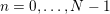 $n=0,\ldots ,N-1$
, will be used for the numerical approximation of (2.24) with step-size
$n=0,\ldots ,N-1$
, will be used for the numerical approximation of (2.24) with step-size
 $\unicode[STIX]{x1D6E5}t:=1/N$
,
$\unicode[STIX]{x1D6E5}t:=1/N$
,
 $t_{n}=n\unicode[STIX]{x1D6E5}t$
. In other words, we replace
$t_{n}=n\unicode[STIX]{x1D6E5}t$
. In other words, we replace
 $Z_{t_{n}}^{+}$
with its numerical approximation
$Z_{t_{n}}^{+}$
with its numerical approximation
 $Z_{n}^{+}$
. A numerical approximation (realization) of the whole solution path
$Z_{n}^{+}$
. A numerical approximation (realization) of the whole solution path
 $z_{[0,1]}$
will be denoted by
$z_{[0,1]}$
will be denoted by
 $z_{0:N}=Z_{0:N}^{+}(\unicode[STIX]{x1D714})$
and can be computed recursively due to the Markov property of the Euler–Maruyama scheme. The marginal PDFs of
$z_{0:N}=Z_{0:N}^{+}(\unicode[STIX]{x1D714})$
and can be computed recursively due to the Markov property of the Euler–Maruyama scheme. The marginal PDFs of
 $Z_{n}^{+}$
are denoted by
$Z_{n}^{+}$
are denoted by
 $\unicode[STIX]{x1D70B}_{n}$
.
$\unicode[STIX]{x1D70B}_{n}$
.
For any finite number of time-steps
 $N$
, we can define a joint PDF
$N$
, we can define a joint PDF
 $\unicode[STIX]{x1D70B}_{0:N}$
on
$\unicode[STIX]{x1D70B}_{0:N}$
on
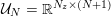 ${\mathcal{U}}_{N}=\mathbb{R}^{N_{z}\times (N+1)}$
via
${\mathcal{U}}_{N}=\mathbb{R}^{N_{z}\times (N+1)}$
via
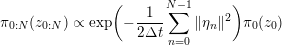 $$\begin{eqnarray}\unicode[STIX]{x1D70B}_{0:N}(z_{0:N})\propto \exp \biggl(-\displaystyle \frac{1}{2\unicode[STIX]{x1D6E5}t}\mathop{\sum }_{n=0}^{N-1}\Vert \unicode[STIX]{x1D702}_{n}\Vert ^{2}\biggr)\unicode[STIX]{x1D70B}_{0}(z_{0})\end{eqnarray}$$
with
 $$\begin{eqnarray}\unicode[STIX]{x1D702}_{n}:=\unicode[STIX]{x1D6FE}^{-1/2}(z_{n+1}-z_{n}-f_{t_{n}}(z_{n})\unicode[STIX]{x1D6E5}t)\end{eqnarray}$$
and
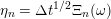 $\unicode[STIX]{x1D702}_{n}=\unicode[STIX]{x1D6E5}t^{1/2}\unicode[STIX]{x1D6EF}_{n}(\unicode[STIX]{x1D714})$
. Note that the joint PDF
$\unicode[STIX]{x1D702}_{n}=\unicode[STIX]{x1D6E5}t^{1/2}\unicode[STIX]{x1D6EF}_{n}(\unicode[STIX]{x1D714})$
. Note that the joint PDF
 $\unicode[STIX]{x1D70B}_{0:N}(z_{0:N})$
can also be expressed in terms of
$\unicode[STIX]{x1D70B}_{0:N}(z_{0:N})$
can also be expressed in terms of
 $z_{0}$
and
$z_{0}$
and
 $\unicode[STIX]{x1D702}_{0:N-1}$
.
$\unicode[STIX]{x1D702}_{0:N-1}$
.
The numerical approximation of SDEs provides an example for which the increase in computational cost for producing
 $L>M$
samples from the PDF
$L>M$
samples from the PDF
 $\unicode[STIX]{x1D70B}_{0:N}$
versus
$\unicode[STIX]{x1D70B}_{0:N}$
versus
 $L=M$
is non-trivial, in general.
$L=M$
is non-trivial, in general.
We now extend Definition 3.1 to the case of temporally discretized SDEs in the form of (3.5).
Definition 3.5. Let us assume that we have
 $L=M$
independent numerical solutions
$L=M$
independent numerical solutions
 $z_{0:N}^{i}$
of (3.5). We introduce an
$z_{0:N}^{i}$
of (3.5). We introduce an
 $M\times M$
matrix
$M\times M$
matrix
 $Q_{n}$
for each
$Q_{n}$
for each
 $n=1,\ldots ,N$
with entries
$n=1,\ldots ,N$
with entries
 $$\begin{eqnarray}q_{lj}=q_{+}(z_{n}^{l}|z_{n-1}^{j}):=\text{n}(z_{n}^{l};z_{n-1}^{j}+\unicode[STIX]{x1D6E5}tf(z_{n-1}^{j}),\unicode[STIX]{x1D6FE}\unicode[STIX]{x1D6E5}t\,I).\end{eqnarray}$$
With each
 $Q_{n}$
we associate a finite-state Markov chain
$Q_{n}$
we associate a finite-state Markov chain
 $Q_{n}^{+}$
as defined by (3.2) for general transition densities
$Q_{n}^{+}$
as defined by (3.2) for general transition densities
 $q_{+}$
in Definition 3.1. An approximation of the Markov transition from time
$q_{+}$
in Definition 3.1. An approximation of the Markov transition from time
 $t_{0}=0$
to
$t_{0}=0$
to
 $t_{1}=1$
is now provided by
$t_{1}=1$
is now provided by
 $$\begin{eqnarray}Q_{+}:=\mathop{\prod }_{n=1}^{N}Q_{n}^{+}.\end{eqnarray}$$
Remark 3.6. The approximation (3.2) can be related to the diffusion map approximation of the infinitesimal generator of Brownian dynamics
 $$\begin{eqnarray}\text{d}Z_{t}^{+}=-\unicode[STIX]{x1D6FB}_{z}U(Z_{t}^{+})\,\text{d}t+\sqrt{2}\,\,\text{d}W_{t}^{+}\end{eqnarray}$$
with potential
 $U(z)=-\log \unicode[STIX]{x1D70B}^{\ast }(z)$
in the following sense. First note that
$U(z)=-\log \unicode[STIX]{x1D70B}^{\ast }(z)$
in the following sense. First note that
 $\unicode[STIX]{x1D70B}^{\ast }$
is invariant under the associated Fokker–Planck equation (2.26) with (time-independent) operator
$\unicode[STIX]{x1D70B}^{\ast }$
is invariant under the associated Fokker–Planck equation (2.26) with (time-independent) operator
 ${\mathcal{L}}^{\dagger }$
written in the form
${\mathcal{L}}^{\dagger }$
written in the form
 $$\begin{eqnarray}{\mathcal{L}}^{\dagger }\unicode[STIX]{x1D70B}=\unicode[STIX]{x1D6FB}_{z}\cdot \biggl(\unicode[STIX]{x1D70B}^{\ast }\unicode[STIX]{x1D6FB}_{z}\displaystyle \frac{\unicode[STIX]{x1D70B}}{\unicode[STIX]{x1D70B}^{\ast }}\biggr).\end{eqnarray}$$
Let
 $z^{i}$
,
$z^{i}$
,
 $i=1,\ldots ,M$
, denote
$i=1,\ldots ,M$
, denote
 $M$
samples from the invariant PDF
$M$
samples from the invariant PDF
 $\unicode[STIX]{x1D70B}^{\ast }$
and define the symmetric matrix
$\unicode[STIX]{x1D70B}^{\ast }$
and define the symmetric matrix
 $Q\in \mathbb{R}^{M\times M}$
with entries
$Q\in \mathbb{R}^{M\times M}$
with entries
 $$\begin{eqnarray}q_{lj}=\text{n}(z^{l};z^{j},2\unicode[STIX]{x1D6E5}t\,I).\end{eqnarray}$$
Then the associated (symmetric) matrix (3.2), as introduced in Definition 3.1, provides a discrete approximation to the evolution of a probability vector
 $p_{0}\propto \unicode[STIX]{x1D70B}_{0}/\unicode[STIX]{x1D70B}^{\ast }$
over a time-interval
$p_{0}\propto \unicode[STIX]{x1D70B}_{0}/\unicode[STIX]{x1D70B}^{\ast }$
over a time-interval
 $\unicode[STIX]{x1D6E5}t$
and, hence, to the semigroup operator
$\unicode[STIX]{x1D6E5}t$
and, hence, to the semigroup operator
 $\text{e}^{\unicode[STIX]{x1D6E5}t{\mathcal{L}}}$
with the infinitesimal generator
$\text{e}^{\unicode[STIX]{x1D6E5}t{\mathcal{L}}}$
with the infinitesimal generator
 ${\mathcal{L}}$
given by
${\mathcal{L}}$
given by
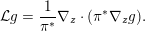 $$\begin{eqnarray}{\mathcal{L}}g=\displaystyle \frac{1}{\unicode[STIX]{x1D70B}^{\ast }}\unicode[STIX]{x1D6FB}_{z}\cdot (\unicode[STIX]{x1D70B}^{\ast }\unicode[STIX]{x1D6FB}_{z}g).\end{eqnarray}$$
We formally obtain
 $$\begin{eqnarray}{\mathcal{L}}\approx \displaystyle \frac{Q_{+}-I}{\unicode[STIX]{x1D6E5}t}\end{eqnarray}$$
for
 $\unicode[STIX]{x1D6E5}t$
sufficiently small. The symmetry of
$\unicode[STIX]{x1D6E5}t$
sufficiently small. The symmetry of
 $Q_{+}$
reflects the fact that
$Q_{+}$
reflects the fact that
 ${\mathcal{L}}$
is self-adjoint with respect to the weighted inner product
${\mathcal{L}}$
is self-adjoint with respect to the weighted inner product
 $$\begin{eqnarray}\langle f,g\rangle _{\unicode[STIX]{x1D70B}^{\ast }}=\int f(z)\,g(z)\,\unicode[STIX]{x1D70B}^{\ast }(z)\,\text{d}z.\end{eqnarray}$$
See Harlim (Reference Harlim2018) for a discussion of alternative diffusion map approximations to the infinitesimal generator
 ${\mathcal{L}}$
and Appendix A.1 for an application to the feedback particle filter formulation of continuous-time data assimilation.
${\mathcal{L}}$
and Appendix A.1 for an application to the feedback particle filter formulation of continuous-time data assimilation.
We also consider the discretization
 $$\begin{eqnarray}Z_{n+1}^{+}=Z_{n}^{+}+(f_{t_{n}}(Z_{n}^{+})+u_{t_{n}}(Z_{n}^{+}))\unicode[STIX]{x1D6E5}t+(\unicode[STIX]{x1D6FE}\unicode[STIX]{x1D6E5}t)^{1/2}\,\unicode[STIX]{x1D6EF}_{n},\end{eqnarray}$$
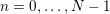 $n=0,\ldots ,N-1$
, of a controlled SDE (2.30) with associated PDF
$n=0,\ldots ,N-1$
, of a controlled SDE (2.30) with associated PDF
 $\unicode[STIX]{x1D70B}_{0:N}^{u}$
defined by
$\unicode[STIX]{x1D70B}_{0:N}^{u}$
defined by
 $$\begin{eqnarray}\unicode[STIX]{x1D70B}_{0:N}^{u}(z_{0:N}^{u})\propto \exp \biggl(-\displaystyle \frac{1}{2\unicode[STIX]{x1D6E5}t}\mathop{\sum }_{n=0}^{N-1}\Vert \unicode[STIX]{x1D702}_{n}^{u}\Vert ^{2}\biggr)\unicode[STIX]{x1D70B}_{0}(z_{0}),\end{eqnarray}$$
where
 $$\begin{eqnarray}\displaystyle \unicode[STIX]{x1D702}_{n}^{u} & := & \displaystyle \unicode[STIX]{x1D6FE}^{-1/2}\{z_{n+1}^{u}-z_{n}^{u}-(f_{t_{n}}(z_{n}^{u})+u_{t_{n}}(z_{n}^{u}))\unicode[STIX]{x1D6E5}t\}\nonumber\\ \displaystyle & = & \displaystyle \unicode[STIX]{x1D702}_{n}-\displaystyle \frac{\unicode[STIX]{x1D6E5}t}{\unicode[STIX]{x1D6FE}^{1/2}}u_{t_{n}}(z_{n}^{u}).\nonumber\end{eqnarray}$$
Here
 $z_{0:N}^{u}$
denotes a realization of the discretization (3.12) with control laws
$z_{0:N}^{u}$
denotes a realization of the discretization (3.12) with control laws
 $u_{t_{n}}$
. We find that
$u_{t_{n}}$
. We find that
 $$\begin{eqnarray}\displaystyle \displaystyle \frac{1}{2\unicode[STIX]{x1D6E5}t}\Vert \unicode[STIX]{x1D702}_{n}^{u}\Vert ^{2} & = & \displaystyle \displaystyle \frac{1}{2\unicode[STIX]{x1D6E5}t}\Vert \unicode[STIX]{x1D702}_{n}\Vert ^{2}-\displaystyle \frac{1}{\unicode[STIX]{x1D6FE}^{1/2}}u_{t_{n}}(z_{n}^{u})^{\text{T}}\unicode[STIX]{x1D702}_{n}+\displaystyle \frac{\unicode[STIX]{x1D6E5}t}{2\unicode[STIX]{x1D6FE}}\Vert u_{t_{n}}(z_{n}^{u})\Vert ^{2}\nonumber\\ \displaystyle & = & \displaystyle \displaystyle \frac{1}{2\unicode[STIX]{x1D6E5}t}\Vert \unicode[STIX]{x1D702}_{n}\Vert ^{2}-\displaystyle \frac{1}{\unicode[STIX]{x1D6FE}^{1/2}}u_{t_{n}}(z_{n}^{u})^{\text{T}}\unicode[STIX]{x1D702}_{n}^{u}-\displaystyle \frac{\unicode[STIX]{x1D6E5}t}{2\unicode[STIX]{x1D6FE}}\Vert u_{t_{n}}(z_{n}^{u})\Vert ^{2},\nonumber\end{eqnarray}$$
and hence
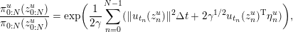 $$\begin{eqnarray}\displaystyle \frac{\unicode[STIX]{x1D70B}_{0:N}^{u}(z_{0:N}^{u})}{\unicode[STIX]{x1D70B}_{0:N}(z_{0:N}^{u})}=\exp \biggl(\displaystyle \frac{1}{2\unicode[STIX]{x1D6FE}}\mathop{\sum }_{n=0}^{N-1}(\Vert u_{t_{n}}(z_{n}^{u})\Vert ^{2}\unicode[STIX]{x1D6E5}t+2\unicode[STIX]{x1D6FE}^{1/2}u_{t_{n}}(z_{n}^{u})^{\text{T}}\unicode[STIX]{x1D702}_{n}^{u})\biggr),\end{eqnarray}$$
which provides a discrete version of (2.33) since
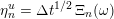 $\unicode[STIX]{x1D702}_{n}^{u}=\unicode[STIX]{x1D6E5}t^{1/2}\,\unicode[STIX]{x1D6EF}_{n}(\unicode[STIX]{x1D714})$
are increments of Brownian motion over time intervals of length
$\unicode[STIX]{x1D702}_{n}^{u}=\unicode[STIX]{x1D6E5}t^{1/2}\,\unicode[STIX]{x1D6EF}_{n}(\unicode[STIX]{x1D714})$
are increments of Brownian motion over time intervals of length
 $\unicode[STIX]{x1D6E5}t$
.
$\unicode[STIX]{x1D6E5}t$
.
Remark 3.7. Instead of discretizing the forward SDE (2.24) in order to produce samples from the forecast PDF
 $\unicode[STIX]{x1D70B}_{1}$
, one can also start from the mean-field formulation (2.29) and its time discretization, for example,
$\unicode[STIX]{x1D70B}_{1}$
, one can also start from the mean-field formulation (2.29) and its time discretization, for example,
 $$\begin{eqnarray}z_{n+1}^{i}=z_{n}^{i}+(f_{t_{n}}(z_{n}^{i})+u_{t_{n}}(z_{n}^{i}))\unicode[STIX]{x1D6E5}t\end{eqnarray}$$
for
 $i=1,\ldots ,M$
and
$i=1,\ldots ,M$
and
 $$\begin{eqnarray}u_{t_{n}}(z)=-\displaystyle \frac{\unicode[STIX]{x1D6FE}}{2}\unicode[STIX]{x1D6FB}_{z}\log \widetilde{\unicode[STIX]{x1D70B}}_{n}(z).\end{eqnarray}$$
Here
 $\widetilde{\unicode[STIX]{x1D70B}}_{n}$
stands for an approximation to the marginal PDF
$\widetilde{\unicode[STIX]{x1D70B}}_{n}$
stands for an approximation to the marginal PDF
 $\unicode[STIX]{x1D70B}_{t_{n}}$
based on the available samples
$\unicode[STIX]{x1D70B}_{t_{n}}$
based on the available samples
 $z_{n}^{i}$
,
$z_{n}^{i}$
,
 $i=1,\ldots ,M$
. A simple approximation is obtained by the Gaussian PDF
$i=1,\ldots ,M$
. A simple approximation is obtained by the Gaussian PDF
 $$\begin{eqnarray}\widetilde{\unicode[STIX]{x1D70B}}_{n}(z)=\text{n}(z;\bar{z}_{n},P_{n}^{zz})\end{eqnarray}$$
with empirical mean
 $$\begin{eqnarray}\bar{z}_{n}=\displaystyle \frac{1}{M}\mathop{\sum }_{i=1}^{M}z_{n}^{i}\end{eqnarray}$$
and empirical covariance matrix
 $$\begin{eqnarray}P_{n}^{zz}=\displaystyle \frac{1}{M-1}\mathop{\sum }_{i=1}^{M}z_{n}^{i}(z_{n}^{i}-\bar{z}_{n})^{\text{T}}.\end{eqnarray}$$
The system (3.15) becomes
 $$\begin{eqnarray}z_{n+1}^{i}=z_{n}^{i}+(f_{t_{n}}(z_{n}^{i})+\unicode[STIX]{x1D6FE}(P_{n}^{zz})^{-1}(z_{n}^{i}-\bar{z}_{n}))\unicode[STIX]{x1D6E5}t,\end{eqnarray}$$
 $i=1,\ldots ,M$
, and provides an example of an interacting particle approximation. Similar mean-field formulations can be found for the backward SDE (2.28).
$i=1,\ldots ,M$
, and provides an example of an interacting particle approximation. Similar mean-field formulations can be found for the backward SDE (2.28).
3.2 Filtering
Let us assume that we are given
 $M$
samples,
$M$
samples,
 $z_{1}^{i}$
, from the forecast PDF using forward transition kernels
$z_{1}^{i}$
, from the forecast PDF using forward transition kernels
 $q_{+}(\cdot \,|z_{0}^{i})$
,
$q_{+}(\cdot \,|z_{0}^{i})$
,
 $i=1,\ldots ,M$
. The likelihood function
$i=1,\ldots ,M$
. The likelihood function
 $l(z)$
leads to importance weights
$l(z)$
leads to importance weights
 $$\begin{eqnarray}w^{i}\propto l(z_{1}^{i}).\end{eqnarray}$$
We also normalize these importance weights such that (2.19) holds.
Remark 3.8. The model evidence
 $\unicode[STIX]{x1D6FD}$
can be estimated from the samples,
$\unicode[STIX]{x1D6FD}$
can be estimated from the samples,
 $z_{1}^{i}$
, and the likelihood
$z_{1}^{i}$
, and the likelihood
 $l(z)$
as follows:
$l(z)$
as follows:
 $$\begin{eqnarray}\widetilde{\unicode[STIX]{x1D6FD}}:=\displaystyle \frac{1}{M}\mathop{\sum }_{i=1}^{M}l(z_{1}^{i}).\end{eqnarray}$$
If the likelihood is of the form
 $$\begin{eqnarray}l(z)\propto \exp \biggl(-\displaystyle \frac{1}{2}(y_{1}-h(z))^{\text{T}}R^{-1} (y_{1}-h(z)\biggr)\end{eqnarray}$$
and the prior distribution in
 $y=h(z)$
can be approximated as being Gaussian with covariance
$y=h(z)$
can be approximated as being Gaussian with covariance
 $$\begin{eqnarray}P^{hh}:=\displaystyle \frac{1}{M-1}\mathop{\sum }_{i=1}^{M}h(z_{1}^{i})(h(z_{1}^{i})-\bar{h})^{\text{T}},\quad \bar{h}:=\displaystyle \frac{1}{M}\mathop{\sum }_{i=1}^{M}h(z_{1}^{i}),\end{eqnarray}$$
then the evidence can be approximated by
 $$\begin{eqnarray}\widetilde{\unicode[STIX]{x1D6FD}}\approx \displaystyle \frac{1}{(2\unicode[STIX]{x1D70B})^{N_{y}/2}|P^{yy}|^{1/2}}\exp \biggl(-\displaystyle \frac{1}{2}(y_{1}-\bar{h})^{\text{T}}(P^{yy})^{-1}(y_{1}-\bar{h})\biggr)\end{eqnarray}$$
with
 $$\begin{eqnarray}P^{yy}:=R+P^{hh}.\end{eqnarray}$$
Such an approximation has been used, for example, in Carrassi, Bocquet, Hannart and Ghil (Reference Carrassi, Bocquet, Hannart and Ghil2017). See also Reich and Cotter (Reference Reich and Cotter2015) for more details on how to compute and use model evidence in the context of sequential data assimilation.
Sequential data assimilation requires that we produce
 $M$
equally weighted samples
$M$
equally weighted samples
 $\widehat{z}_{1}^{j}\sim \widehat{\unicode[STIX]{x1D70B}}_{1}$
from the
$\widehat{z}_{1}^{j}\sim \widehat{\unicode[STIX]{x1D70B}}_{1}$
from the
 $M$
weighted samples
$M$
weighted samples
 $z_{1}^{i}\sim \unicode[STIX]{x1D70B}_{1}$
with weights
$z_{1}^{i}\sim \unicode[STIX]{x1D70B}_{1}$
with weights
 $w^{i}$
. This is a standard problem in Monte Carlo integration and there are many ways to tackle this problem, among which are multinomial, residual, systematic and stratified resampling (Douc and Cappe Reference Douc and Cappe2005). Here we focus on those resampling methods which are based on a discrete Markov chain
$w^{i}$
. This is a standard problem in Monte Carlo integration and there are many ways to tackle this problem, among which are multinomial, residual, systematic and stratified resampling (Douc and Cappe Reference Douc and Cappe2005). Here we focus on those resampling methods which are based on a discrete Markov chain
 $P\in \mathbb{R}^{M\times M}$
with the property that
$P\in \mathbb{R}^{M\times M}$
with the property that
 $$\begin{eqnarray}w=\displaystyle \frac{1}{M}P\,\unicode[STIX]{x1D7D9}_{M},\quad w=\biggl(\displaystyle \frac{w^{1}}{M},\ldots ,\displaystyle \frac{w^{M}}{M}\biggr)^{\text{T}}.\end{eqnarray}$$
The Markov property of
 $P$
implies that
$P$
implies that
 $P^{\text{T}}\unicode[STIX]{x1D7D9}_{M}=\unicode[STIX]{x1D7D9}_{M}$
. We now consider the set of all Markov chains
$P^{\text{T}}\unicode[STIX]{x1D7D9}_{M}=\unicode[STIX]{x1D7D9}_{M}$
. We now consider the set of all Markov chains
 $\unicode[STIX]{x1D6F1}_{\text{M}}$
, as defined by (3.3), with
$\unicode[STIX]{x1D6F1}_{\text{M}}$
, as defined by (3.3), with
 $p_{1}=w$
. Any Markov chain
$p_{1}=w$
. Any Markov chain
 $P\in \unicode[STIX]{x1D6F1}_{\text{M}}$
can now be used for resampling, but we seek the Markov chain
$P\in \unicode[STIX]{x1D6F1}_{\text{M}}$
can now be used for resampling, but we seek the Markov chain
 $P^{\ast }\in \unicode[STIX]{x1D6F1}_{\text{M}}$
which minimizes the expected distance between the samples, that is,
$P^{\ast }\in \unicode[STIX]{x1D6F1}_{\text{M}}$
which minimizes the expected distance between the samples, that is,
 $$\begin{eqnarray}P^{\ast }=\arg \min _{P\in \unicode[STIX]{x1D6F1}_{\text{M}}}\mathop{\sum }_{i,j=1}^{M}p_{ij}\Vert z_{1}^{i}-z_{1}^{j}\Vert ^{2}.\end{eqnarray}$$
Note that (3.18) is a special case of the optimal transport problem (2.36) with the involved probability measures being discrete measures. Resampling can now be performed according to
 $$\begin{eqnarray}\mathbb{P}[\widehat{Z}_{1}^{j}(\unicode[STIX]{x1D714})=z_{1}^{i}]=p_{ij}^{\ast }\end{eqnarray}$$
for
 $j=1,\ldots ,M$
.
$j=1,\ldots ,M$
.
Since it is known that (3.18) converges to (2.36) as
 $M\rightarrow \infty$
(McCann Reference McCann1995) and since (2.36) leads to a transformation (2.38), the resampling step (3.19) has been replaced by
$M\rightarrow \infty$
(McCann Reference McCann1995) and since (2.36) leads to a transformation (2.38), the resampling step (3.19) has been replaced by
 $$\begin{eqnarray}\widehat{z}_{1}^{j}=\mathop{\sum }_{i=1}^{M}z_{1}^{i}\,p_{ij}^{\ast }\end{eqnarray}$$
in the so-called ensemble transform particle filter (ETPF) (Reich Reference Reich2013, Reich and Cotter Reference Reich and Cotter2015). In other words, the ETPF replaces resampling with probabilities
 $p_{ij}^{\ast }$
by its mean (3.20) for each
$p_{ij}^{\ast }$
by its mean (3.20) for each
 $j=1,\ldots ,M$
. The ETPF leads to a biased approximation to the resampling step which is consistent in the limit
$j=1,\ldots ,M$
. The ETPF leads to a biased approximation to the resampling step which is consistent in the limit
 $M\rightarrow \infty$
.
$M\rightarrow \infty$
.
The general formulation (3.20) with the coefficients
 $p_{ij}^{\ast }$
chosen appropriatelyFootnote
2
leads to a large class of so-called ensemble transform particle filters (Reich and Cotter Reference Reich and Cotter2015). Ensemble transform particle filters generally result in biased and inconsistent but robust estimates, which have found applications to high-dimensional state space models (Evensen Reference Evensen2006, Vetra-Carvalho et al.
Reference Vetra-Carvalho, van Leeuwen, Nerger, Barth, Altaf, Brasseur, Kirchgessner and Beckers2018) for which traditional particle filters fail due to the ‘curse of dimensionality’ (Bengtsson, Bickel and Li Reference Bengtsson, Bickel and Li2008). More specifically, the class of ensemble transform particle filters includes the popular ensemble Kalman filters (Evensen Reference Evensen2006, Reich and Cotter Reference Reich and Cotter2015, Vetra-Carvalho et al.
Reference Vetra-Carvalho, van Leeuwen, Nerger, Barth, Altaf, Brasseur, Kirchgessner and Beckers2018, Carrassi, Bocquet, Bertino and Evensen Reference Carrassi, Bocquet, Bertino and Evensen2018) and so-called second-order accurate particle filters with coefficients
$p_{ij}^{\ast }$
chosen appropriatelyFootnote
2
leads to a large class of so-called ensemble transform particle filters (Reich and Cotter Reference Reich and Cotter2015). Ensemble transform particle filters generally result in biased and inconsistent but robust estimates, which have found applications to high-dimensional state space models (Evensen Reference Evensen2006, Vetra-Carvalho et al.
Reference Vetra-Carvalho, van Leeuwen, Nerger, Barth, Altaf, Brasseur, Kirchgessner and Beckers2018) for which traditional particle filters fail due to the ‘curse of dimensionality’ (Bengtsson, Bickel and Li Reference Bengtsson, Bickel and Li2008). More specifically, the class of ensemble transform particle filters includes the popular ensemble Kalman filters (Evensen Reference Evensen2006, Reich and Cotter Reference Reich and Cotter2015, Vetra-Carvalho et al.
Reference Vetra-Carvalho, van Leeuwen, Nerger, Barth, Altaf, Brasseur, Kirchgessner and Beckers2018, Carrassi, Bocquet, Bertino and Evensen Reference Carrassi, Bocquet, Bertino and Evensen2018) and so-called second-order accurate particle filters with coefficients
 $p_{ij}^{\ast }$
in (3.20) chosen such that the weighted ensemble mean
$p_{ij}^{\ast }$
in (3.20) chosen such that the weighted ensemble mean
 $$\begin{eqnarray}\bar{z}_{1}:=\displaystyle \frac{1}{M}\mathop{\sum }_{i=1}^{M}w^{i}z_{1}^{i}\end{eqnarray}$$
and the weighted ensemble covariance matrix
 $$\begin{eqnarray}\widetilde{P}^{zz}:=\displaystyle \frac{1}{M}\mathop{\sum }_{i=1}^{M}w^{i}(z_{1}^{i}-\bar{z}_{1})(z_{1}^{i}-\bar{z}_{1})^{\text{T}}\end{eqnarray}$$
are exactly reproduced by the transformed and equally weighted particles
 $\widehat{z}_{1}^{j}$
,
$\widehat{z}_{1}^{j}$
,
 $j=1,\ldots ,M$
, defined by (3.20), that is,
$j=1,\ldots ,M$
, defined by (3.20), that is,
 $$\begin{eqnarray}\displaystyle \frac{1}{M}\mathop{\sum }_{j=1}^{M}\widehat{z}_{1}^{j}=\bar{z}_{1},\quad \displaystyle \frac{1}{M-1}\mathop{\sum }_{j=1}^{M}(\widehat{z}_{1}^{i}-\bar{z}_{1})(\widehat{z}_{1}^{i}-\bar{z}_{1})^{\text{T}}=\widetilde{P}^{zz}.\end{eqnarray}$$
See the survey paper by Vetra-Carvalho et al. (Reference Vetra-Carvalho, van Leeuwen, Nerger, Barth, Altaf, Brasseur, Kirchgessner and Beckers2018) and the paper by Acevedo et al. (Reference Acevedo, de Wiljes and Reich2017) for more details. A summary of the ensemble Kalman filter can be found in Appendix A.3.
In addition, hybrid methods (Frei and Künsch Reference Frei and Künsch2013, Chustagulprom, Reich and Reinhardt Reference Chustagulprom, Reich and Reinhardt2016), which bridge between classical particle filters and the ensemble Kalman filter, have recently been successfully applied to atmospheric fluid dynamics (Robert, Leuenberger and Künsch Reference Robert, Leuenberger and Künsch2018).
Remark 3.9. Another approach for transforming samples,
 $z_{1}^{i}$
, from the forecast PDF
$z_{1}^{i}$
, from the forecast PDF
 $\unicode[STIX]{x1D70B}_{1}$
into samples,
$\unicode[STIX]{x1D70B}_{1}$
into samples,
 $\widehat{z}_{1}^{i}$
, from the filtering PDF
$\widehat{z}_{1}^{i}$
, from the filtering PDF
 $\widehat{\unicode[STIX]{x1D70B}}_{1}$
is provided through the mean-field interpretation
$\widehat{\unicode[STIX]{x1D70B}}_{1}$
is provided through the mean-field interpretation
 $$\begin{eqnarray}\displaystyle \frac{\text{d}}{\text{d}s}\breve{Z}_{s}=-\unicode[STIX]{x1D6FB}_{z}\log \displaystyle \frac{\breve{\unicode[STIX]{x1D70B}}_{s}(\breve{Z}_{s})}{\widehat{\unicode[STIX]{x1D70B}}_{1}(\breve{Z}_{s})}\end{eqnarray}$$
of the Fokker–Planck equation (2.26) for a random variable
 $\breve{Z}_{s}$
with law
$\breve{Z}_{s}$
with law
 $\breve{\unicode[STIX]{x1D70B}}_{s}$
, drift term
$\breve{\unicode[STIX]{x1D70B}}_{s}$
, drift term
 $f_{s}(z)=\unicode[STIX]{x1D6FB}_{z}\log \widehat{\unicode[STIX]{x1D70B}}_{1}$
and
$f_{s}(z)=\unicode[STIX]{x1D6FB}_{z}\log \widehat{\unicode[STIX]{x1D70B}}_{1}$
and
 $\unicode[STIX]{x1D6FE}=2$
, that is,
$\unicode[STIX]{x1D6FE}=2$
, that is,
 $$\begin{eqnarray}\unicode[STIX]{x2202}_{s}\breve{\unicode[STIX]{x1D70B}}_{s}=\unicode[STIX]{x1D6FB}_{z}\cdot \biggl(\breve{\unicode[STIX]{x1D70B}}_{s}\unicode[STIX]{x1D6FB}_{z}\log \displaystyle \frac{\breve{\unicode[STIX]{x1D70B}}_{s}}{\widehat{\unicode[STIX]{x1D70B}}_{1}}\biggr)\end{eqnarray}$$
in artificial time
 $s\geq 0$
. It holds under fairly general assumptions that
$s\geq 0$
. It holds under fairly general assumptions that
 $$\begin{eqnarray}\lim _{s\rightarrow \infty }\breve{\unicode[STIX]{x1D70B}}_{s}=\widehat{\unicode[STIX]{x1D70B}}_{1}\end{eqnarray}$$
(Pavliotis Reference Pavliotis2014) and one can set
 $\breve{\unicode[STIX]{x1D70B}}_{0}=\unicode[STIX]{x1D70B}_{1}$
. The more common approach would be to solve Brownian dynamics
$\breve{\unicode[STIX]{x1D70B}}_{0}=\unicode[STIX]{x1D70B}_{1}$
. The more common approach would be to solve Brownian dynamics
 $$\begin{eqnarray}\,\text{d}\breve{Z}_{s}=\unicode[STIX]{x1D6FB}_{z}\log \widehat{\unicode[STIX]{x1D70B}}_{1}(Z_{s})\,\text{d}t+\sqrt{2}\,\text{d}W_{s}^{+}\end{eqnarray}$$
for each sample
 $z_{1}^{i}$
from
$z_{1}^{i}$
from
 $\unicode[STIX]{x1D70B}_{1}$
, i.e.
$\unicode[STIX]{x1D70B}_{1}$
, i.e.
 $\breve{Z}_{0}(\unicode[STIX]{x1D714})=z_{1}^{i}$
,
$\breve{Z}_{0}(\unicode[STIX]{x1D714})=z_{1}^{i}$
,
 $i=1,\ldots ,M$
, at initial time and
$i=1,\ldots ,M$
, at initial time and
 $$\begin{eqnarray}\widehat{z}_{1}^{i}=\lim _{s\rightarrow \infty }\breve{Z}_{s}(\unicode[STIX]{x1D714}).\end{eqnarray}$$
In other words, formulation (3.21) replaces stochastic Brownian dynamics with a deterministic interacting particle system. See Appendix A.1 and Remark 4.3 for further details.
3.3 Smoothing
Recall that the joint smoothing distribution
 $\widehat{\unicode[STIX]{x1D70B}}(z_{0},z_{1})$
can be represented in the form (2.47) with modified transition kernel (2.10) and smoothing distribution (2.8) at time
$\widehat{\unicode[STIX]{x1D70B}}(z_{0},z_{1})$
can be represented in the form (2.47) with modified transition kernel (2.10) and smoothing distribution (2.8) at time
 $t_{0}$
with weights
$t_{0}$
with weights
 $\unicode[STIX]{x1D6FE}^{i}$
determined by (2.9).
$\unicode[STIX]{x1D6FE}^{i}$
determined by (2.9).
Let us assume that it is possible to sample from
 $\widehat{q}_{+}(z_{1}|z_{0}^{i})$
and that the weights
$\widehat{q}_{+}(z_{1}|z_{0}^{i})$
and that the weights
 $\unicode[STIX]{x1D6FE}^{i}$
are available. Then we can utilize (2.47) in sequential data assimilation as follows. We first resample the
$\unicode[STIX]{x1D6FE}^{i}$
are available. Then we can utilize (2.47) in sequential data assimilation as follows. We first resample the
 $z_{0}^{i}$
at time
$z_{0}^{i}$
at time
 $t_{0}$
using a discrete Markov chain
$t_{0}$
using a discrete Markov chain
 $P\in \mathbb{R}^{M\times M}$
satisfying
$P\in \mathbb{R}^{M\times M}$
satisfying
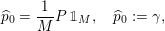 $$\begin{eqnarray}\widehat{p}_{0}=\displaystyle \frac{1}{M}P\,\unicode[STIX]{x1D7D9}_{M},\quad \widehat{p}_{0}:=\unicode[STIX]{x1D6FE},\end{eqnarray}$$
with
 $\unicode[STIX]{x1D6FE}$
defined in (2.12). Again optimal transportation can be used to identify a suitable
$\unicode[STIX]{x1D6FE}$
defined in (2.12). Again optimal transportation can be used to identify a suitable
 $P$
. More explicitly, we now consider the set of all Markov chains
$P$
. More explicitly, we now consider the set of all Markov chains
 $\unicode[STIX]{x1D6F1}_{\text{M}}$
, as defined by (3.3), with
$\unicode[STIX]{x1D6F1}_{\text{M}}$
, as defined by (3.3), with
 $p_{1}=\unicode[STIX]{x1D6FE}$
. Then the Markov chain
$p_{1}=\unicode[STIX]{x1D6FE}$
. Then the Markov chain
 $P^{\ast }$
arising from the associated optimal transport problem (3.18) can be used for resampling, that is,
$P^{\ast }$
arising from the associated optimal transport problem (3.18) can be used for resampling, that is,
 $$\begin{eqnarray}\mathbb{P}[\widetilde{Z}_{0}^{j}(\unicode[STIX]{x1D714})=z_{0}^{i}]=p_{ij}^{\ast }.\end{eqnarray}$$
Once equally weighted samples
 $\widehat{z}_{0}^{i}$
,
$\widehat{z}_{0}^{i}$
,
 $i=1,\ldots ,M$
, from
$i=1,\ldots ,M$
, from
 $\widehat{\unicode[STIX]{x1D70B}}_{0}$
have been determined, the desired samples
$\widehat{\unicode[STIX]{x1D70B}}_{0}$
have been determined, the desired samples
 $\widehat{z}_{1}^{i}$
from
$\widehat{z}_{1}^{i}$
from
 $\widehat{\unicode[STIX]{x1D70B}}_{1}$
are simply given by
$\widehat{\unicode[STIX]{x1D70B}}_{1}$
are simply given by
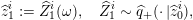 $$\begin{eqnarray}\widehat{z}_{1}^{i}:=\widehat{Z}_{1}^{i}(\unicode[STIX]{x1D714}),\quad \widehat{Z}_{1}^{i}\sim \widehat{q}_{+}(\cdot \,|\widehat{z}_{0}^{i}),\end{eqnarray}$$
for
 $i=1,\ldots ,M$
.
$i=1,\ldots ,M$
.
The required transition kernels (2.10) are explicitly available for state space models with Gaussian model errors and Gaussian likelihood functions. In many other cases, these kernels are not explicitly available or are difficult to draw from. In such cases, one can resort to sample-based transition kernels.
For example, consider the twisted discrete Markov kernel (3.4) with twisting potential
 $\unicode[STIX]{x1D713}(z)=l(z)$
. The associated vector
$\unicode[STIX]{x1D713}(z)=l(z)$
. The associated vector
 $v$
from (3.4) then gives rise to a probability vector
$v$
from (3.4) then gives rise to a probability vector
 $\widehat{p}_{0}=c\,v\in \mathbb{R}^{M}$
with
$\widehat{p}_{0}=c\,v\in \mathbb{R}^{M}$
with
 $c>0$
an appropriate scaling factor, and
$c>0$
an appropriate scaling factor, and
 $$\begin{eqnarray}\widehat{p}_{1}:=Q_{+}^{\unicode[STIX]{x1D713}}\widehat{p}_{0}\end{eqnarray}$$
approximates the filtering distribution at time
 $t_{1}$
. The Markov transition matrix
$t_{1}$
. The Markov transition matrix
 $Q_{+}^{\unicode[STIX]{x1D713}}\in \mathbb{R}^{L\times M}$
together with
$Q_{+}^{\unicode[STIX]{x1D713}}\in \mathbb{R}^{L\times M}$
together with
 $\widehat{p}_{0}$
provides an approximation to the smoothing kernel
$\widehat{p}_{0}$
provides an approximation to the smoothing kernel
 $\widehat{q}_{+}(z_{1}|z_{0})$
and
$\widehat{q}_{+}(z_{1}|z_{0})$
and
 $\widehat{\unicode[STIX]{x1D70B}}_{0}$
, respectively.
$\widehat{\unicode[STIX]{x1D70B}}_{0}$
, respectively.
The approximations
 $Q_{+}^{\unicode[STIX]{x1D713}}\in \mathbb{R}^{L\times M}$
and
$Q_{+}^{\unicode[STIX]{x1D713}}\in \mathbb{R}^{L\times M}$
and
 $\widehat{p}_{0}\in \mathbb{R}^{M}$
can be used to first generate equally weighted samples
$\widehat{p}_{0}\in \mathbb{R}^{M}$
can be used to first generate equally weighted samples
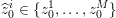 $\widehat{z}_{0}^{i}\in \{z_{0}^{1},\ldots ,z_{0}^{M}\}$
with distribution
$\widehat{z}_{0}^{i}\in \{z_{0}^{1},\ldots ,z_{0}^{M}\}$
with distribution
 $\widehat{p}_{0}$
via, for example, resampling with replacement. If
$\widehat{p}_{0}$
via, for example, resampling with replacement. If
 $\widehat{z}_{0}^{i}=z_{0}^{k}$
for an index
$\widehat{z}_{0}^{i}=z_{0}^{k}$
for an index
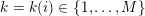 $k=k(i)\in \{1,\ldots ,M\}$
, then
$k=k(i)\in \{1,\ldots ,M\}$
, then
 $$\begin{eqnarray}\mathbb{P}[\widehat{Z}_{1}^{i}(\unicode[STIX]{x1D714})=z_{1}^{l}]=(Q_{+}^{\unicode[STIX]{x1D713}})_{lk}\end{eqnarray}$$
for each
 $i=1,\ldots ,M$
. The
$i=1,\ldots ,M$
. The
 $\widehat{z}_{1}^{i}$
are equally weighted samples from the discrete filtering distribution
$\widehat{z}_{1}^{i}$
are equally weighted samples from the discrete filtering distribution
 $\widehat{p}_{1}$
, which is an approximation to the continuous filtering PDF
$\widehat{p}_{1}$
, which is an approximation to the continuous filtering PDF
 $\widehat{\unicode[STIX]{x1D70B}}_{1}$
.
$\widehat{\unicode[STIX]{x1D70B}}_{1}$
.
Remark 3.10. One has to take computational complexity and robustness into account when deciding whether to utilize methods from Section 3.2 or this subsection to advance
 $M$
samples
$M$
samples
 $z_{0}^{i}$
from the prior distribution
$z_{0}^{i}$
from the prior distribution
 $\unicode[STIX]{x1D70B}_{0}$
into
$\unicode[STIX]{x1D70B}_{0}$
into
 $M$
samples
$M$
samples
 $\widehat{z}_{1}^{i}$
from the posterior distribution
$\widehat{z}_{1}^{i}$
from the posterior distribution
 $\widehat{\unicode[STIX]{x1D70B}}_{1}$
. While the methods from Section 3.2 are easier to implement, the methods of this subsection benefit from the fact that
$\widehat{\unicode[STIX]{x1D70B}}_{1}$
. While the methods from Section 3.2 are easier to implement, the methods of this subsection benefit from the fact that
 $$\begin{eqnarray}M>\displaystyle \frac{1}{\Vert \unicode[STIX]{x1D6FE}\Vert ^{2}}\geq \displaystyle \frac{1}{\Vert w\Vert ^{2}}\geq 1,\end{eqnarray}$$
in general, where the importance weights
 $\unicode[STIX]{x1D6FE}\in \mathbb{R}^{M}$
and
$\unicode[STIX]{x1D6FE}\in \mathbb{R}^{M}$
and
 $w\in \mathbb{R}^{M}$
are defined in (2.12) and (3.17), respectively. In other words, the methods from this subsection lead to larger effective sample sizes (Liu Reference Liu2001, Agapiou et al.
Reference Agapiou, Papaspipliopoulos, Sanz-Alonso and Stuart2017).
$w\in \mathbb{R}^{M}$
are defined in (2.12) and (3.17), respectively. In other words, the methods from this subsection lead to larger effective sample sizes (Liu Reference Liu2001, Agapiou et al.
Reference Agapiou, Papaspipliopoulos, Sanz-Alonso and Stuart2017).
Remark 3.11. We mention that finding efficient methods for solving the more general smoothing problem (2.2) is an active area of research. See, for example, the recent contributions by Guarniero et al. (Reference Guarniero, Johansen and Lee2017) and Heng et al. (Reference Heng, Bishop, Deligiannidis and Doucet2018) for discrete-time Markov processes, and Kappen and Ruiz (Reference Kappen and Ruiz2016) as well as Ruiz and Kappen (Reference Ruiz and Kappen2017) for smoothing in the context of SDEs. Ensemble transform methods of the form (3.20) can also be extended to the general smoothing problem. See, for example, Evensen (Reference Evensen2006) and Carrassi et al. (Reference Carrassi, Bocquet, Bertino and Evensen2018) for extensions of the ensemble Kalman filter, and Kirchgessner, Tödter, Ahrens and Nerger (Reference Kirchgessner, Tödter, Ahrens and Nerger2017) for an extension of the nonlinear ensemble transform filter to the smoothing problem.
3.3.1 SDE models (cont.)
After discretization in time, smoothing leads to a change from the forecast PDF (3.6) to
 $$\begin{eqnarray}\displaystyle \widehat{\unicode[STIX]{x1D70B}}_{0:N}(z_{0:N}) & := & \displaystyle \displaystyle \frac{l(z_{N})\unicode[STIX]{x1D70B}_{0:N}(z_{0:N})}{\unicode[STIX]{x1D70B}_{0:N}[l]}\nonumber\\ \displaystyle & \propto & \displaystyle \exp \biggl(-\displaystyle \frac{1}{2\unicode[STIX]{x1D6E5}t}\mathop{\sum }_{n=0}^{N-1}\Vert \unicode[STIX]{x1D709}_{n}\Vert ^{2}\biggr)\unicode[STIX]{x1D70B}_{0}(z_{0})\,l(z_{N})\nonumber\end{eqnarray}$$
with
 $\unicode[STIX]{x1D709}_{n}$
given by (3.7), or, alternatively,
$\unicode[STIX]{x1D709}_{n}$
given by (3.7), or, alternatively,
 $$\begin{eqnarray}\displaystyle \frac{\widehat{\unicode[STIX]{x1D70B}}_{0:N}}{\unicode[STIX]{x1D70B}_{0:N}}(z_{0:N})=\displaystyle \frac{l(z_{N})}{\unicode[STIX]{x1D70B}_{0:N}[l]}.\end{eqnarray}$$
Remark 3.12. Efficient MCMC methods for sampling high-dimensional smoothing distributions can be found in Beskos et al. (Reference Beskos, Girolami, Lan, Farrell and Stuart2017) and Beskos, Pinski, Sanz-Serna and Stuart (Reference Beskos, Pinski, Sanz-Serna and Stuart2011). Improved sampling can also be achieved by using regularized Störmer–Verlet time-stepping methods (Reich and Hundertmark Reference Reich and Hundertmark2011) in a hybrid Monte Carlo method (Liu Reference Liu2001). See Appendix A.2 for more details.
3.4 Schrödinger problem
Recall that the Schrödinger system (2.58)–(2.61) reduces in our context to solving equations (2.64)–(2.65) for the unknown coefficients
 $\unicode[STIX]{x1D6FC}^{i}$
,
$\unicode[STIX]{x1D6FC}^{i}$
,
 $i=1,\ldots ,M$
. In order to make this problem tractable we need to replace the required expectation values with respect to
$i=1,\ldots ,M$
. In order to make this problem tractable we need to replace the required expectation values with respect to
 $q_{+}(z_{1}|z_{0}^{j})$
by Monte Carlo approximations. More specifically, let us assume that we have
$q_{+}(z_{1}|z_{0}^{j})$
by Monte Carlo approximations. More specifically, let us assume that we have
 $L\geq M$
samples
$L\geq M$
samples
 $z_{1}^{l}$
from the forecast PDF
$z_{1}^{l}$
from the forecast PDF
 $\unicode[STIX]{x1D70B}_{1}$
. The associated
$\unicode[STIX]{x1D70B}_{1}$
. The associated
 $L\times M$
matrix
$L\times M$
matrix
 $Q$
with entries (3.1) provides a discrete approximation to the underlying Markov process defined by
$Q$
with entries (3.1) provides a discrete approximation to the underlying Markov process defined by
 $q_{+}(z_{1}|z_{0})$
and initial PDF (2.3).
$q_{+}(z_{1}|z_{0})$
and initial PDF (2.3).
The importance weights in the associated approximation to the filtering distribution
 $$\begin{eqnarray}\widehat{\unicode[STIX]{x1D70B}}_{1}(z)=\displaystyle \frac{1}{L}\mathop{\sum }_{l=1}^{L}w^{l}\,\unicode[STIX]{x1D6FF}(z-z_{1}^{l})\end{eqnarray}$$
are given by (3.16) with the weights normalized such that
 $$\begin{eqnarray}\mathop{\sum }_{l=1}^{L}w^{l}=L.\end{eqnarray}$$
Finding the coefficients
 $\{\unicode[STIX]{x1D6FC}^{i}\}$
in (2.64)–(2.65) can now be reformulated as finding two vectors
$\{\unicode[STIX]{x1D6FC}^{i}\}$
in (2.64)–(2.65) can now be reformulated as finding two vectors
 $u\in \mathbb{R}^{L}$
and
$u\in \mathbb{R}^{L}$
and
 $v\in \mathbb{R}^{M}$
such that
$v\in \mathbb{R}^{M}$
such that
 $$\begin{eqnarray}P^{\ast }:=D(u)QD(v)^{-1}\end{eqnarray}$$
satisfies
 $P^{\ast }\in \unicode[STIX]{x1D6F1}_{\text{M}}$
with
$P^{\ast }\in \unicode[STIX]{x1D6F1}_{\text{M}}$
with
 $p_{1}=w$
in (3.3), that is, more explicitly
$p_{1}=w$
in (3.3), that is, more explicitly
 $$\begin{eqnarray}\unicode[STIX]{x1D6F1}_{\text{M}}=\bigg\{P\in \mathbb{R}^{L\times M}:\,p_{lj}\geq 0,\,\mathop{\sum }_{l=1}^{L}p_{lj}=1,\,\displaystyle \frac{1}{M}\mathop{\sum }_{j=1}^{M}p_{lj}=\displaystyle \frac{w^{l}}{L}\bigg\}.\end{eqnarray}$$
We note that (3.26) are discrete approximations to (2.67) and (2.68), respectively. The scaling factor
 $\widehat{\unicode[STIX]{x1D713}}$
in (2.58) is approximated by the vector
$\widehat{\unicode[STIX]{x1D713}}$
in (2.58) is approximated by the vector
 $v$
up to a normalization constant, while the vector
$v$
up to a normalization constant, while the vector
 $u$
provides an approximation to
$u$
provides an approximation to
 $\unicode[STIX]{x1D713}$
in (2.59). Finally, the desired approximations to the Schrödinger transition kernels
$\unicode[STIX]{x1D713}$
in (2.59). Finally, the desired approximations to the Schrödinger transition kernels
 $q_{+}^{\ast }(z_{1}|z_{0}^{i})$
,
$q_{+}^{\ast }(z_{1}|z_{0}^{i})$
,
 $i=1,\ldots ,M$
, are provided by the columns of
$i=1,\ldots ,M$
, are provided by the columns of
 $P^{\ast }$
, that is,
$P^{\ast }$
, that is,
 $$\begin{eqnarray}\mathbb{P}[\widehat{Z}_{1}^{i}(\unicode[STIX]{x1D714})=z_{1}^{l}]=p_{li}^{\ast }\end{eqnarray}$$
characterizes the desired equally weighted samples
 $\widehat{z}_{1}^{i}$
,
$\widehat{z}_{1}^{i}$
,
 $i=1,\ldots ,M$
, from the filtering distribution
$i=1,\ldots ,M$
, from the filtering distribution
 $\widehat{\unicode[STIX]{x1D70B}}_{1}$
. See the following subsection for more details.
$\widehat{\unicode[STIX]{x1D70B}}_{1}$
. See the following subsection for more details.
The required vectors
 $u$
and
$u$
and
 $v$
can be computed using the iterative Sinkhorn algorithm (2.74)–(2.76) (Cuturi Reference Cuturi and Burges2013, Peyre and Cuturi Reference Peyre and Cuturi2018).
$v$
can be computed using the iterative Sinkhorn algorithm (2.74)–(2.76) (Cuturi Reference Cuturi and Burges2013, Peyre and Cuturi Reference Peyre and Cuturi2018).
Remark 3.13. Note that one can replace the forward transition kernel
 $q_{+}(z_{1}|z_{0})$
in (3.1) with any suitable twisted prediction kernel (1.2). This results in a modified matrix
$q_{+}(z_{1}|z_{0})$
in (3.1) with any suitable twisted prediction kernel (1.2). This results in a modified matrix
 $Q$
in (3.25) and weights
$Q$
in (3.25) and weights
 $w^{l}$
in 3.26. The resulting matrix (3.25) still provides an approximation to the Schrödinger problem.
$w^{l}$
in 3.26. The resulting matrix (3.25) still provides an approximation to the Schrödinger problem.
Remark 3.14. The approximation (3.25) can be extended to an approximation of the Schrödinger forward transition kernels (2.66) in the following sense. We use
 $\unicode[STIX]{x1D6FC}^{i}=1/v_{i}$
in (2.66) and note that the resulting approximation satisfies (2.68) while (2.67) now longer holds exactly. However, since the entries
$\unicode[STIX]{x1D6FC}^{i}=1/v_{i}$
in (2.66) and note that the resulting approximation satisfies (2.68) while (2.67) now longer holds exactly. However, since the entries
 $u_{l}$
of the vector
$u_{l}$
of the vector
 $u$
appearing in (3.25) satisfy
$u$
appearing in (3.25) satisfy
 $$\begin{eqnarray}u_{l}=\displaystyle \frac{w^{l}}{L}\displaystyle \frac{1}{\mathop{\sum }_{j=1}^{M}q_{+}(z_{1}^{l}|z_{0}^{j})/v_{j}},\end{eqnarray}$$
it follows that
 $$\begin{eqnarray}\displaystyle \int q_{+}^{\ast }(z_{1}|z_{0}^{i})\,\text{d}z_{1} & {\approx} & \displaystyle \displaystyle \frac{1}{L}\mathop{\sum }_{l=1}^{L}\displaystyle \frac{l(z_{1}^{l})}{\unicode[STIX]{x1D6FD}}\displaystyle \frac{q_{+}(z_{1}^{l}|z_{0}^{i})/v_{i}}{\mathop{\sum }_{j=1}^{M}q_{+}(z_{1}^{l}|z_{0}^{j})/v_{j}}\nonumber\\ \displaystyle & {\approx} & \displaystyle \displaystyle \frac{1}{L}\mathop{\sum }_{l=1}^{L}w^{l}\displaystyle \frac{q_{+}(z_{1}^{l}|z_{0}^{i})/v_{i}}{\mathop{\sum }_{j=1}^{M}q_{+}(z_{1}^{l}|z_{0}^{j})/v_{j}}=\mathop{\sum }_{l=1}^{L}p_{li}^{\ast }=1.\nonumber\end{eqnarray}$$
Furthermore, one can use such continuous approximations in combination with Monte Carlo sampling methods which do not require normalized target PDFs.
3.4.1 Gaussian model errors (cont.)
One can easily generate
 $L$
,
$L$
,
 $L\geq M$
, i.i.d. samples
$L\geq M$
, i.i.d. samples
 $z_{1}^{l}$
from the forecast PDF (2.21), that is,
$z_{1}^{l}$
from the forecast PDF (2.21), that is,
 $$\begin{eqnarray}Z_{1}^{l}\sim \displaystyle \frac{1}{M}\mathop{\sum }_{j=1}^{M}\text{n}(\cdot \,;\unicode[STIX]{x1D6F9}(z_{0}^{j}),\unicode[STIX]{x1D6FE}B),\end{eqnarray}$$
and with the filtering distribution
 $\widehat{\unicode[STIX]{x1D70B}}_{1}$
characterized through the importance weights (3.16).
$\widehat{\unicode[STIX]{x1D70B}}_{1}$
characterized through the importance weights (3.16).
We define the distance matrix
 $D\in \mathbb{R}^{L\times M}$
with entries
$D\in \mathbb{R}^{L\times M}$
with entries
 $$\begin{eqnarray}d_{lj}:=\displaystyle \frac{1}{2}\Vert z_{1}^{l}-\unicode[STIX]{x1D6F9}(z_{0}^{j})\Vert _{B}^{2},\quad \Vert z\Vert _{B}^{2}:=z^{\text{T}}B^{-1}z,\end{eqnarray}$$
and the matrix
 $Q\in \mathbb{R}^{L\times M}$
with entries
$Q\in \mathbb{R}^{L\times M}$
with entries
 $$\begin{eqnarray}q_{lj}:=\text{e}^{-d_{lj}/\unicode[STIX]{x1D6FE}}.\end{eqnarray}$$
The Markov chain
 $P^{\ast }\in \mathbb{R}^{L\times M}$
is now given by
$P^{\ast }\in \mathbb{R}^{L\times M}$
is now given by
 $$\begin{eqnarray}P^{\ast }=\arg \min _{P\in \unicode[STIX]{x1D6F1}_{\text{M}}}\text{KL}(P||Q)\end{eqnarray}$$
with the set
 $\unicode[STIX]{x1D6F1}_{\text{M}}$
defined by (3.26).
$\unicode[STIX]{x1D6F1}_{\text{M}}$
defined by (3.26).
Once
 $P^{\ast }$
has been computed, the desired Schrödinger transitions from
$P^{\ast }$
has been computed, the desired Schrödinger transitions from
 $\unicode[STIX]{x1D70B}_{0}$
to
$\unicode[STIX]{x1D70B}_{0}$
to
 $\widehat{\unicode[STIX]{x1D70B}}_{1}$
can be represented as follows. The Schrödinger transition kernels
$\widehat{\unicode[STIX]{x1D70B}}_{1}$
can be represented as follows. The Schrödinger transition kernels
 $q_{+}^{\ast }(z_{1}|z_{0}^{i})$
are approximated for each
$q_{+}^{\ast }(z_{1}|z_{0}^{i})$
are approximated for each
 $z_{0}^{i}$
by
$z_{0}^{i}$
by
 $$\begin{eqnarray}\tilde{q}_{+}^{\ast }(z_{1}|z_{0}^{i}):=\mathop{\sum }_{l=1}^{L}p_{li}^{\ast }\,\unicode[STIX]{x1D6FF}(z_{1}-z_{1}^{l}),\quad i=1,\ldots ,M.\end{eqnarray}$$
The empirical measure in (3.27) converges weakly to the desired
 $q_{+}^{\ast }(z_{1}|z_{0}^{i})$
as
$q_{+}^{\ast }(z_{1}|z_{0}^{i})$
as
 $L\rightarrow \infty$
and
$L\rightarrow \infty$
and
 $$\begin{eqnarray}\widehat{\unicode[STIX]{x1D70B}}_{1}(z_{1})\approx \displaystyle \frac{1}{M}\mathop{\sum }_{i=1}^{M}\unicode[STIX]{x1D6FF}(z-\widehat{z}_{1}^{i}),\end{eqnarray}$$
with
 $$\begin{eqnarray}\widehat{z}_{1}^{i}=\widehat{Z}_{1}^{i}(\unicode[STIX]{x1D714}),\quad \widehat{Z}_{1}^{i}\sim \tilde{q}_{+}^{\ast }(\cdot \,|z_{0}^{i}),\end{eqnarray}$$
provides the desired approximation of
 $\widehat{\unicode[STIX]{x1D70B}}_{1}$
by
$\widehat{\unicode[STIX]{x1D70B}}_{1}$
by
 $M$
equally weighted particles
$M$
equally weighted particles
 $\widehat{z}_{1}^{i}$
,
$\widehat{z}_{1}^{i}$
,
 $i=1,\ldots ,M$
.
$i=1,\ldots ,M$
.
We remark that (3.27) has been used to produce the Schrödinger transition kernels for Example 2.5 and Figure 2.3(b) in particular. More specifically, we have
 $M=11$
and used
$M=11$
and used
 $L=11\,000$
. Since the particles
$L=11\,000$
. Since the particles
 $z_{1}^{l}\in \mathbb{R}$
,
$z_{1}^{l}\in \mathbb{R}$
,
 $l=1,\ldots ,L$
, are distributed according to the forecast PDF
$l=1,\ldots ,L$
, are distributed according to the forecast PDF
 $\unicode[STIX]{x1D70B}_{1}$
, a function representation of
$\unicode[STIX]{x1D70B}_{1}$
, a function representation of
 $\tilde{q}_{+}^{\ast }(z_{1}|z_{0}^{i})$
over all of
$\tilde{q}_{+}^{\ast }(z_{1}|z_{0}^{i})$
over all of
 $\mathbb{R}$
is provided by interpolating
$\mathbb{R}$
is provided by interpolating
 $p_{li}^{\ast }$
onto
$p_{li}^{\ast }$
onto
 $\mathbb{R}$
and multiplication of this interpolated function by
$\mathbb{R}$
and multiplication of this interpolated function by
 $\unicode[STIX]{x1D70B}_{1}(z)$
.
$\unicode[STIX]{x1D70B}_{1}(z)$
.
For
 $\unicode[STIX]{x1D6FE}\ll 1$
, the measure in (3.27) can also be approximated by a Gaussian measure with mean
$\unicode[STIX]{x1D6FE}\ll 1$
, the measure in (3.27) can also be approximated by a Gaussian measure with mean
 $$\begin{eqnarray}\bar{z}_{1}^{i}:=\mathop{\sum }_{l=1}^{L}z_{1}^{l}p_{li}^{\ast }\end{eqnarray}$$
and covariance matrix
 $\unicode[STIX]{x1D6FE}B$
, that is, we replace (3.28) with
$\unicode[STIX]{x1D6FE}B$
, that is, we replace (3.28) with
 $$\begin{eqnarray}\widehat{Z}_{1}^{i}\sim \text{N}(\bar{z}_{1}^{i},\unicode[STIX]{x1D6FE}B)\end{eqnarray}$$
for
 $i=1,\ldots ,M$
.
$i=1,\ldots ,M$
.
3.4.2 SDE (cont.)
One can also apply (3.25) in order to approximate the Schrödinger problem associated with SDE models. We typically use
 $L=M$
in this case and utilize (3.8) in place of
$L=M$
in this case and utilize (3.8) in place of
 $Q$
in (3.25). The set
$Q$
in (3.25). The set
 $\unicode[STIX]{x1D6F1}_{\text{M}}$
is still given by (3.26).
$\unicode[STIX]{x1D6F1}_{\text{M}}$
is still given by (3.26).
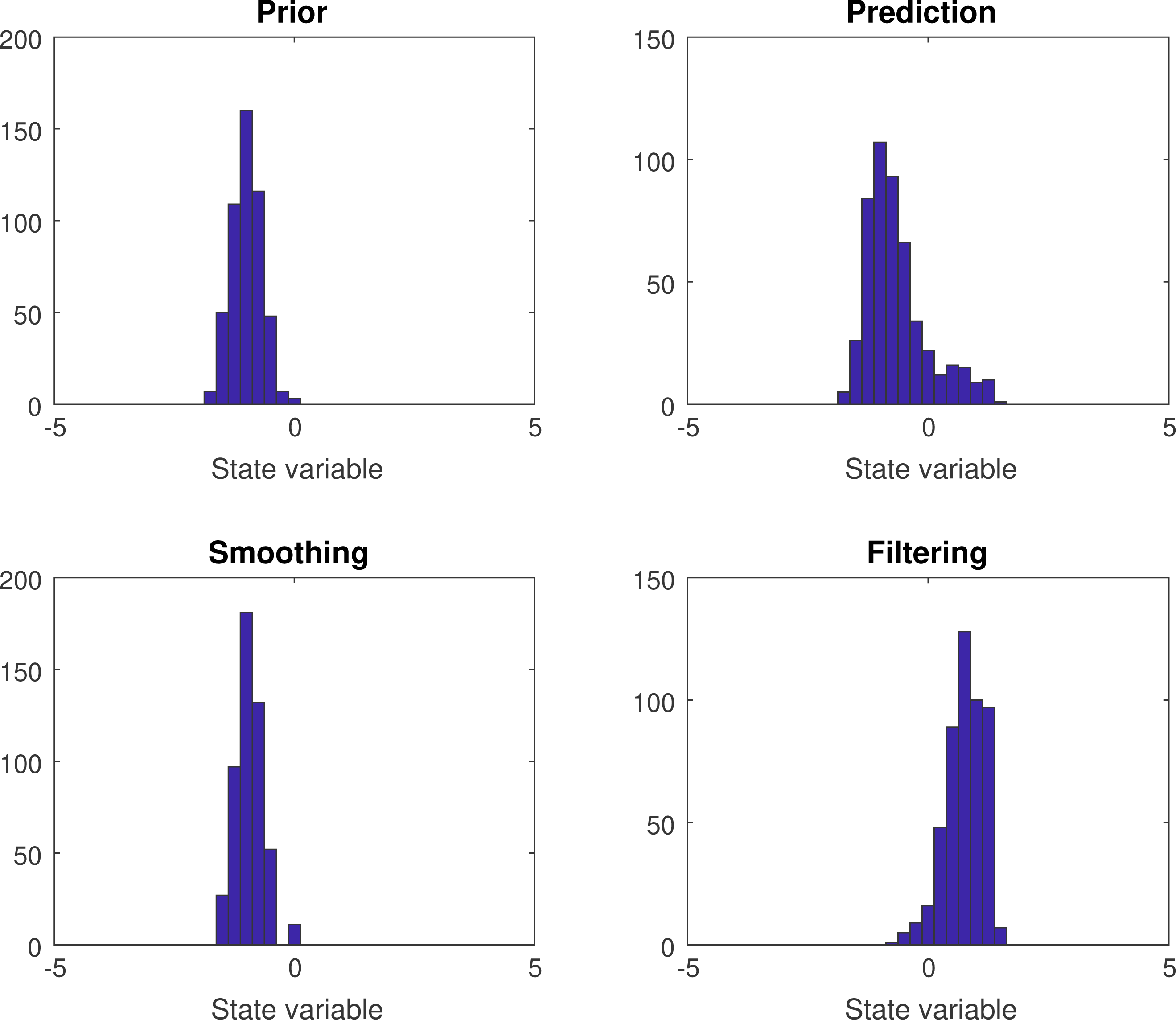
Figure 3.1. Histograms produced from
 $M=200$
Monte Carlo samples of the initial PDF
$M=200$
Monte Carlo samples of the initial PDF
 $\unicode[STIX]{x1D70B}_{0}$
, the forecast PDF
$\unicode[STIX]{x1D70B}_{0}$
, the forecast PDF
 $\unicode[STIX]{x1D70B}_{2}$
at time
$\unicode[STIX]{x1D70B}_{2}$
at time
 $t=2$
, the filtering distribution
$t=2$
, the filtering distribution
 $\widehat{\unicode[STIX]{x1D70B}}_{2}$
at time
$\widehat{\unicode[STIX]{x1D70B}}_{2}$
at time
 $t=2$
, and the smoothing PDF
$t=2$
, and the smoothing PDF
 $\widehat{\unicode[STIX]{x1D70B}}_{0}$
at time
$\widehat{\unicode[STIX]{x1D70B}}_{0}$
at time
 $t=0$
for a Brownian particle moving in a double well potential.
$t=0$
for a Brownian particle moving in a double well potential.
Example 3.15. We consider scalar-valued motion of a Brownian particle in a bimodal potential, that is,
 $$\begin{eqnarray}\,\text{d}Z_{t}^{+}=Z_{t}^{+}\,\text{d}t-(Z_{t}^{+})^{3}\,\text{d}t+\unicode[STIX]{x1D6FE}^{1/2}\,\text{d}W_{t}^{+}\end{eqnarray}$$
with
 $\unicode[STIX]{x1D6FE}=0.5$
and initial distribution
$\unicode[STIX]{x1D6FE}=0.5$
and initial distribution
 $Z_{0}\sim \text{N}(-1,0.3)$
. At time
$Z_{0}\sim \text{N}(-1,0.3)$
. At time
 $t=2$
we measure the location
$t=2$
we measure the location
 $y=1$
with measurement error variance
$y=1$
with measurement error variance
 $R=0.2$
. We simulate the dynamics using
$R=0.2$
. We simulate the dynamics using
 $M=200$
particles and a time-step of
$M=200$
particles and a time-step of
 $\unicode[STIX]{x1D6E5}t=0.01$
in the Euler–Maruyama discretization (3.5). One can find histograms produced from the Monte Carlo samples in Figure 3.1. The samples from the filtering and smoothing distributions are obtained by resampling with replacement from the weighted distributions with weights given by (3.16). Next we compute (3.8) from the
$\unicode[STIX]{x1D6E5}t=0.01$
in the Euler–Maruyama discretization (3.5). One can find histograms produced from the Monte Carlo samples in Figure 3.1. The samples from the filtering and smoothing distributions are obtained by resampling with replacement from the weighted distributions with weights given by (3.16). Next we compute (3.8) from the
 $M=200$
Monte Carlo samples of (3.29). Eleven out of the 200 transition kernels from
$M=200$
Monte Carlo samples of (3.29). Eleven out of the 200 transition kernels from
 $\unicode[STIX]{x1D70B}_{0}$
to
$\unicode[STIX]{x1D70B}_{0}$
to
 $\unicode[STIX]{x1D70B}_{2}$
(prediction problem) and
$\unicode[STIX]{x1D70B}_{2}$
(prediction problem) and
 $\unicode[STIX]{x1D70B}_{0}$
to
$\unicode[STIX]{x1D70B}_{0}$
to
 $\widehat{\unicode[STIX]{x1D70B}}_{2}$
(Schrödinger problem) are displayed in Figure 3.2.
$\widehat{\unicode[STIX]{x1D70B}}_{2}$
(Schrödinger problem) are displayed in Figure 3.2.
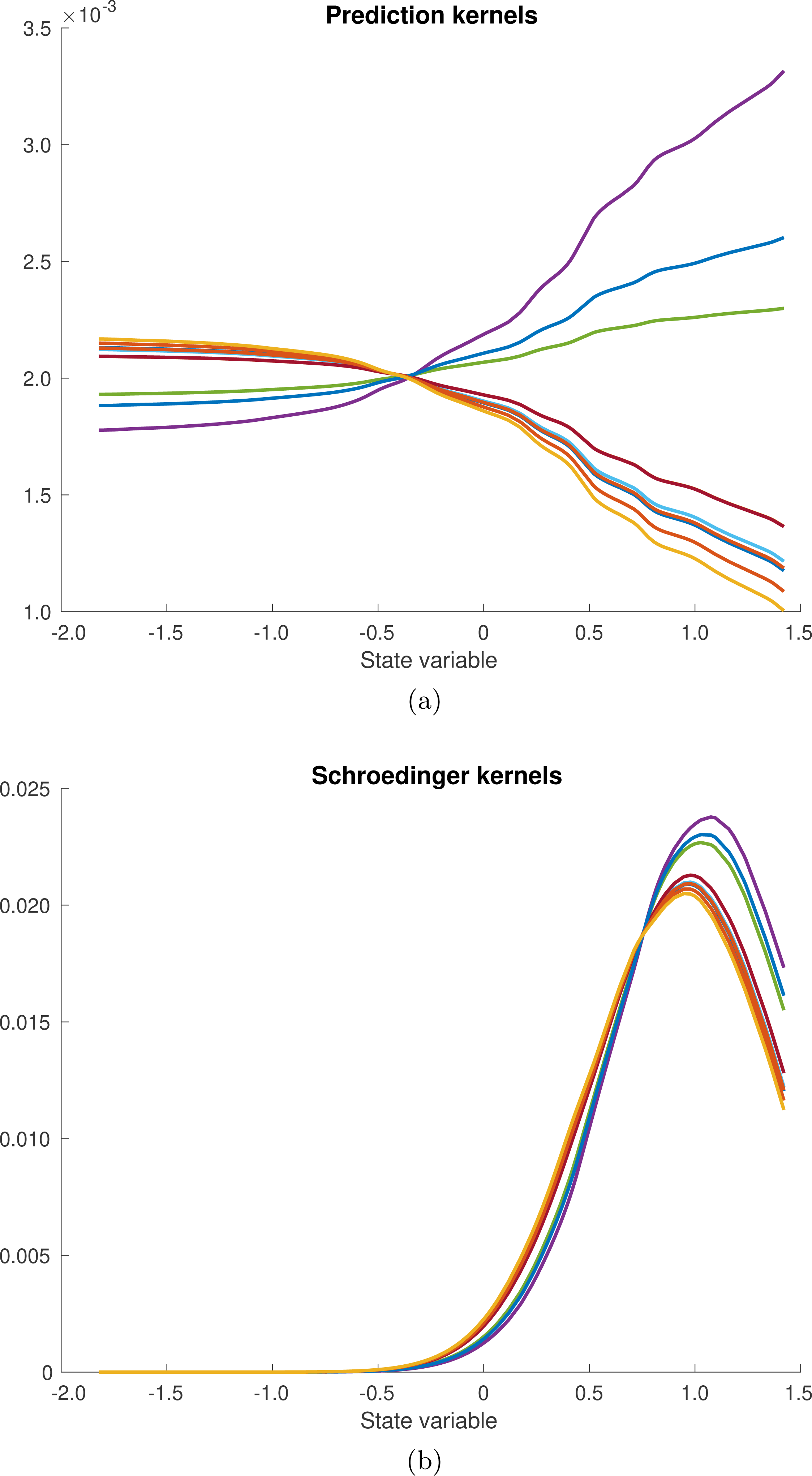
Figure 3.2. (a) Approximations of typical transition kernels from time
 $\unicode[STIX]{x1D70B}_{0}$
to
$\unicode[STIX]{x1D70B}_{0}$
to
 $\unicode[STIX]{x1D70B}_{2}$
under the Brownian dynamics model (3.29). (b) Approximations of typical Schrödinger transition kernels from
$\unicode[STIX]{x1D70B}_{2}$
under the Brownian dynamics model (3.29). (b) Approximations of typical Schrödinger transition kernels from
 $\unicode[STIX]{x1D70B}_{0}$
to
$\unicode[STIX]{x1D70B}_{0}$
to
 $\widehat{\unicode[STIX]{x1D70B}}_{2}$
. All approximations were computed using the Sinkhorn algorithm and by linear interpolation between the
$\widehat{\unicode[STIX]{x1D70B}}_{2}$
. All approximations were computed using the Sinkhorn algorithm and by linear interpolation between the
 $M=200$
data points.
$M=200$
data points.
The Sinkhorn approach requires relatively large sample sizes
 $M$
in order to lead to useful approximations. Alternatively we may assume that there is an approximative control term
$M$
in order to lead to useful approximations. Alternatively we may assume that there is an approximative control term
 $u_{t}^{(0)}$
with associated forward SDE
$u_{t}^{(0)}$
with associated forward SDE
 $$\begin{eqnarray}\,\text{d}Z_{t}^{+}=f_{t}(Z_{t})\,\text{d}t+u_{t}^{(0)}(Z_{t}^{+})\,\text{d}t+\unicode[STIX]{x1D6FE}^{1/2}\,\text{d}W_{t}^{+},\quad t\in [0,1],\end{eqnarray}$$
and
 $Z_{0}^{+}\sim \unicode[STIX]{x1D70B}_{0}$
. We denote the associated path measure by
$Z_{0}^{+}\sim \unicode[STIX]{x1D70B}_{0}$
. We denote the associated path measure by
 $\mathbb{Q}^{(0)}$
. Girsanov’s theorem implies that the Radon–Nikodym derivative of
$\mathbb{Q}^{(0)}$
. Girsanov’s theorem implies that the Radon–Nikodym derivative of
 $\mathbb{Q}$
with respect to
$\mathbb{Q}$
with respect to
 $\mathbb{Q}^{(0)}$
is given by (compare (2.33))
$\mathbb{Q}^{(0)}$
is given by (compare (2.33))
 $$\begin{eqnarray}\displaystyle \frac{\text{d}\mathbb{Q}}{\text{d}\mathbb{Q}^{(0)}}_{|z_{[0,1]}^{(0)}}=\exp (-V^{(0)}),\end{eqnarray}$$
where
 $V^{(0)}$
is defined via the stochastic integral
$V^{(0)}$
is defined via the stochastic integral
 $$\begin{eqnarray}V^{(0)}:=\displaystyle \frac{1}{2\unicode[STIX]{x1D6FE}}\int _{0}^{1}(\Vert u_{t}^{(0)}\Vert ^{2}\,\text{d}t+2\unicode[STIX]{x1D6FE}^{1/2}u_{t}^{(0)}\cdot \,\text{d}W_{t}^{+})\end{eqnarray}$$
along solution paths
 $z_{[0,1]}^{(0)}$
of (3.30). Because of
$z_{[0,1]}^{(0)}$
of (3.30). Because of
 $$\begin{eqnarray}\displaystyle \frac{\text{d}\widehat{\mathbb{P}}}{\text{d}\mathbb{Q}^{(0)}}_{|z_{[0,1]}^{(0)}}=\displaystyle \frac{\text{d}\widehat{\mathbb{P}}}{\text{d}\mathbb{Q}}_{|z_{[0,1]}^{(0)}}\,\displaystyle \frac{\text{d}\mathbb{Q}}{\text{d}\mathbb{Q}^{(0)}}_{|z_{[0,1]}^{(0)}}\propto l(z_{1}^{(0)})\,\exp (-V^{(0)}),\end{eqnarray}$$
we can now use (3.30) to importance-sample from the filtering PDF
 $\widehat{\unicode[STIX]{x1D70B}}_{1}$
. The control
$\widehat{\unicode[STIX]{x1D70B}}_{1}$
. The control
 $u_{t}^{(0)}$
should be chosen such that the variance in the modified likelihood function
$u_{t}^{(0)}$
should be chosen such that the variance in the modified likelihood function
 $$\begin{eqnarray}l^{(0)}(z_{[0,1]}^{(0)}):=l(z_{1}^{(0)})\,\exp (-V^{(0)})\end{eqnarray}$$
is reduced compared to the uncontrolled case
 $u_{t}^{(0)}\equiv 0$
. In particular, the filter distribution
$u_{t}^{(0)}\equiv 0$
. In particular, the filter distribution
 $\widehat{\unicode[STIX]{x1D70B}}_{1}$
at time
$\widehat{\unicode[STIX]{x1D70B}}_{1}$
at time
 $t=1$
satisfies
$t=1$
satisfies
 $$\begin{eqnarray}\widehat{\unicode[STIX]{x1D70B}}_{1}(z_{1}^{(0)})\propto l^{(0)}(z_{[0,1]}^{(0)})\,\unicode[STIX]{x1D70B}_{1}^{(0)}(z_{1}^{(0)}),\end{eqnarray}$$
where
 $\unicode[STIX]{x1D70B}_{t}^{(0)}$
,
$\unicode[STIX]{x1D70B}_{t}^{(0)}$
,
 $t\in (0,1]$
, denote the marginal PDFs generated by (3.30).
$t\in (0,1]$
, denote the marginal PDFs generated by (3.30).
We now describe an iterative algorithm for the associated Schrödinger problem in the spirit of the Sinkhorn iteration from Section 2.3.2.
Lemma 3.16. The desired optimal control law can be computed iteratively,
 $$\begin{eqnarray}u_{t}^{(k+1)}=u_{t}^{(k)}+\unicode[STIX]{x1D6FE}\unicode[STIX]{x1D6FB}_{z}\log \unicode[STIX]{x1D713}_{t}^{(k)},\quad k=0,1,\ldots ,\end{eqnarray}$$
for given
 $u_{t}^{(k)}$
and the potential
$u_{t}^{(k)}$
and the potential
 $\unicode[STIX]{x1D713}_{t}^{(k)}$
obtained as the solutions to the backward Kolmogorov equation
$\unicode[STIX]{x1D713}_{t}^{(k)}$
obtained as the solutions to the backward Kolmogorov equation
 $$\begin{eqnarray}\unicode[STIX]{x2202}_{t}\unicode[STIX]{x1D713}_{t}^{(k)}=-{\mathcal{L}}_{t}^{(k)}\unicode[STIX]{x1D713}_{t}^{(k)},\quad {\mathcal{L}}_{t}^{(k)}g:=\unicode[STIX]{x1D6FB}_{z}g\cdot (f_{t}+u_{t}^{(k)})+\displaystyle \frac{\unicode[STIX]{x1D6FE}}{2}\unicode[STIX]{x1D6E5}_{z}g,\end{eqnarray}$$
with final time condition
 $$\begin{eqnarray}\unicode[STIX]{x1D713}_{1}^{(k)}(z):=\displaystyle \frac{\widehat{\unicode[STIX]{x1D70B}}_{1}(z)}{\unicode[STIX]{x1D70B}_{1}^{(k)}(z)}.\end{eqnarray}$$
Here
 $\unicode[STIX]{x1D70B}_{1}^{(k)}$
denotes the time-one marginal of the path measure
$\unicode[STIX]{x1D70B}_{1}^{(k)}$
denotes the time-one marginal of the path measure
 $\mathbb{Q}^{(k)}$
induced by (2.30) with control term
$\mathbb{Q}^{(k)}$
induced by (2.30) with control term
 $u_{t}=u_{t}^{(k)}$
and initial PDF
$u_{t}=u_{t}^{(k)}$
and initial PDF
 $\unicode[STIX]{x1D70B}_{0}$
. The recursion (3.32) is stopped whenever the final time condition (3.34) is sufficiently close to a constant function.
$\unicode[STIX]{x1D70B}_{0}$
. The recursion (3.32) is stopped whenever the final time condition (3.34) is sufficiently close to a constant function.
Proof. The extension of the Sinkhorn algorithm to continuous PDFs and its convergence has been discussed by Chen, Georgiou and Pavon (Reference Chen, Georgiou and Pavon2016a ).◻
Remark 3.17. Note that
 $\unicode[STIX]{x1D713}_{t}^{(k)}$
needs to be determined up to a constant of proportionality only since the associated control law is determined from
$\unicode[STIX]{x1D713}_{t}^{(k)}$
needs to be determined up to a constant of proportionality only since the associated control law is determined from
 $\unicode[STIX]{x1D713}_{t}^{(k)}$
by (3.32). One can also replace (3.33) with any other method for solving the smoothing problem associated to the SDE (2.30) with
$\unicode[STIX]{x1D713}_{t}^{(k)}$
by (3.32). One can also replace (3.33) with any other method for solving the smoothing problem associated to the SDE (2.30) with
 $Z_{0}^{+}\sim \unicode[STIX]{x1D70B}_{0}$
, control law
$Z_{0}^{+}\sim \unicode[STIX]{x1D70B}_{0}$
, control law
 $u_{t}=u_{t}^{(k)}$
, and likelihood function
$u_{t}=u_{t}^{(k)}$
, and likelihood function
 $l(z)=\unicode[STIX]{x1D713}_{1}^{(k)}(z)$
. See Appendix A.4 for a forward–backward SDE formulation in particular.
$l(z)=\unicode[STIX]{x1D713}_{1}^{(k)}(z)$
. See Appendix A.4 for a forward–backward SDE formulation in particular.
We need to restrict the class of possible control laws
 $u_{t}^{(k)}$
in order to obtain a computationally feasible implementations in practice. For example, a simple class of control laws is provided by linear controls of the form
$u_{t}^{(k)}$
in order to obtain a computationally feasible implementations in practice. For example, a simple class of control laws is provided by linear controls of the form
 $$\begin{eqnarray}u_{t}^{(k)}(z)=-B_{t}^{(k)}(z-m_{t}^{(k)})\end{eqnarray}$$
with appropriately chosen symmetric positive definite matrices
 $B_{t}^{(k)}$
and vectors
$B_{t}^{(k)}$
and vectors
 $m_{t}^{(k)}$
. Such approximations can, for example, be obtained from the smoother extensions of ensemble transform methods mentioned earlier. See also the recent work by Kappen and Ruiz (Reference Kappen and Ruiz2016) and Ruiz and Kappen (Reference Ruiz and Kappen2017) on numerical methods for the SDE smoothing problem.
$m_{t}^{(k)}$
. Such approximations can, for example, be obtained from the smoother extensions of ensemble transform methods mentioned earlier. See also the recent work by Kappen and Ruiz (Reference Kappen and Ruiz2016) and Ruiz and Kappen (Reference Ruiz and Kappen2017) on numerical methods for the SDE smoothing problem.
4 DA for continuous-time data
In this section we focus on the continuous-time filtering problem over the time interval
 $[0,1]$
, that is, on the assimilation of data that arrive continuously in time. If one is only interested in transforming samples from the prior distribution at
$[0,1]$
, that is, on the assimilation of data that arrive continuously in time. If one is only interested in transforming samples from the prior distribution at
 $t=0$
into samples of the filtering distribution at time
$t=0$
into samples of the filtering distribution at time
 $t=1$
, then all methods from the previous sections can be applied once the associated filtering distribution
$t=1$
, then all methods from the previous sections can be applied once the associated filtering distribution
 $\widehat{\unicode[STIX]{x1D70B}}_{1}$
is available. However, it is more natural to consider the associated filtering distributions
$\widehat{\unicode[STIX]{x1D70B}}_{1}$
is available. However, it is more natural to consider the associated filtering distributions
 $\widehat{\unicode[STIX]{x1D70B}}_{t}$
for all
$\widehat{\unicode[STIX]{x1D70B}}_{t}$
for all
 $t\in (0,1]$
and to derive appropriate transformations in the form of mean-field equations in continuous time. We distinguish between smooth and non-smooth data
$t\in (0,1]$
and to derive appropriate transformations in the form of mean-field equations in continuous time. We distinguish between smooth and non-smooth data
 $y_{t}$
,
$y_{t}$
,
 $t\in [0,1]$
.
$t\in [0,1]$
.
4.1 Smooth data
We start from a forward SDE model (2.24) with associated path measure
 $\mathbb{Q}$
over the space of continuous functions
$\mathbb{Q}$
over the space of continuous functions
 ${\mathcal{C}}$
. However, contrary to the previous sections, the likelihood
${\mathcal{C}}$
. However, contrary to the previous sections, the likelihood
 $l$
is defined along a whole solution path
$l$
is defined along a whole solution path
 $z_{[0,1]}$
as follows:
$z_{[0,1]}$
as follows:
 $$\begin{eqnarray}\displaystyle \frac{\text{d}\widehat{\mathbb{P}}}{\text{d}\mathbb{Q}}_{|z_{[0,1]}}\propto l(z_{[0,1]}),\quad l(z_{[0,1]}):=\exp \biggl(-\int _{0}^{1}V_{t}(z_{t})\,\text{d}t\biggr)\end{eqnarray}$$
with the assumption that
 $\mathbb{Q}[l]<\infty$
and
$\mathbb{Q}[l]<\infty$
and
 $V_{t}(z)\geq 0$
. A specific example of a suitable
$V_{t}(z)\geq 0$
. A specific example of a suitable
 $V_{t}$
is provided by
$V_{t}$
is provided by
 $$\begin{eqnarray}V_{t}(z)=\displaystyle \frac{1}{2}\Vert h(z)-y_{t}\Vert ^{2},\end{eqnarray}$$
where the data function
 $y_{t}\in \mathbb{R}$
,
$y_{t}\in \mathbb{R}$
,
 $t\in [0,1]$
, is a smooth function of time and
$t\in [0,1]$
, is a smooth function of time and
 $h(z)$
is a forward operator connecting the model states to the observations/data. The associated estimation problem has, for example, been addressed by Mortensen (Reference Mortensen1968) and Fleming (Reference Fleming1997) from an optimal control perspective and has led to what is called the minimum energy estimator. Recall that the filtering PDF
$h(z)$
is a forward operator connecting the model states to the observations/data. The associated estimation problem has, for example, been addressed by Mortensen (Reference Mortensen1968) and Fleming (Reference Fleming1997) from an optimal control perspective and has led to what is called the minimum energy estimator. Recall that the filtering PDF
 $\widehat{\unicode[STIX]{x1D70B}}_{1}$
is the marginal PDF of
$\widehat{\unicode[STIX]{x1D70B}}_{1}$
is the marginal PDF of
 $\widehat{\mathbb{P}}$
at time
$\widehat{\mathbb{P}}$
at time
 $t=1$
.
$t=1$
.
The associated time-continuous smoothing/filtering problems are based on the time-dependent path measures
 $\widehat{\mathbb{P}}_{t}$
defined by
$\widehat{\mathbb{P}}_{t}$
defined by
 $$\begin{eqnarray}\displaystyle \frac{\text{d}\widehat{\mathbb{P}}_{t}}{\text{d}\mathbb{Q}}_{|z_{[0,1]}}\propto l(z_{[0,t]}),\quad l(z_{[0,t]}):=\exp \biggl(-\int _{0}^{t}V_{s}(z_{s})\,\text{d}s\biggr)\end{eqnarray}$$
for
 $t\in (0,1]$
. We let
$t\in (0,1]$
. We let
 $\widehat{\unicode[STIX]{x1D70B}}_{t}$
denote the marginal PDF of
$\widehat{\unicode[STIX]{x1D70B}}_{t}$
denote the marginal PDF of
 $\widehat{\mathbb{P}}_{t}$
at time
$\widehat{\mathbb{P}}_{t}$
at time
 $t$
. Note that
$t$
. Note that
 $\widehat{\unicode[STIX]{x1D70B}}_{t}$
is the filtering PDF, i.e. the marginal PDF at time
$\widehat{\unicode[STIX]{x1D70B}}_{t}$
is the filtering PDF, i.e. the marginal PDF at time
 $t$
conditioned on all the data available until time
$t$
conditioned on all the data available until time
 $t$
. Also note that
$t$
. Also note that
 $\widehat{\unicode[STIX]{x1D70B}}_{t}$
is different from the marginal (smoothing) PDF of
$\widehat{\unicode[STIX]{x1D70B}}_{t}$
is different from the marginal (smoothing) PDF of
 $\widehat{\mathbb{P}}$
at time
$\widehat{\mathbb{P}}$
at time
 $t$
.
$t$
.
We now state a modified Fokker–Planck equation which describes the time evolution of the filtering PDFs
 $\widehat{\unicode[STIX]{x1D70B}}_{t}$
.
$\widehat{\unicode[STIX]{x1D70B}}_{t}$
.
Lemma 4.1. The marginal distributions
 $\widehat{\unicode[STIX]{x1D70B}}_{t}$
of
$\widehat{\unicode[STIX]{x1D70B}}_{t}$
of
 $\widehat{\mathbb{P}}_{t}$
satisfy the modified Fokker–Planck equation
$\widehat{\mathbb{P}}_{t}$
satisfy the modified Fokker–Planck equation
 $$\begin{eqnarray}\unicode[STIX]{x2202}_{t}\widehat{\unicode[STIX]{x1D70B}}_{t}={\mathcal{L}}_{t}^{\dagger }\widehat{\unicode[STIX]{x1D70B}}_{t}-\widehat{\unicode[STIX]{x1D70B}}_{t}(V_{t}-\widehat{\unicode[STIX]{x1D70B}}_{t}[V_{t}])\end{eqnarray}$$
with
 ${\mathcal{L}}_{t}^{\dagger }$
defined by (2.25).
${\mathcal{L}}_{t}^{\dagger }$
defined by (2.25).
Proof. This can be seen by setting
 $\unicode[STIX]{x1D6FE}=0$
and
$\unicode[STIX]{x1D6FE}=0$
and
 $f_{t}\equiv 0$
in (2.24) for simplicity and by considering the incremental change of measure induced by the likelihood, that is,
$f_{t}\equiv 0$
in (2.24) for simplicity and by considering the incremental change of measure induced by the likelihood, that is,
 $$\begin{eqnarray}\displaystyle \frac{\widehat{\unicode[STIX]{x1D70B}}_{t+\unicode[STIX]{x1D6FF}t}}{\widehat{\unicode[STIX]{x1D70B}}_{t}}\propto \text{e}^{-V_{t}\unicode[STIX]{x1D6FF}t}\approx 1-V_{t}\,\unicode[STIX]{x1D6FF}t,\end{eqnarray}$$
and taking the limit
 $\unicode[STIX]{x1D6FF}t\rightarrow 0$
under the constraint that
$\unicode[STIX]{x1D6FF}t\rightarrow 0$
under the constraint that
 $\widehat{\unicode[STIX]{x1D70B}}_{t}[1]=1$
is preserved.◻
$\widehat{\unicode[STIX]{x1D70B}}_{t}[1]=1$
is preserved.◻
We now derive a mean-field interpretation of (4.2) and rewrite (4.2) in the form
 $$\begin{eqnarray}\unicode[STIX]{x2202}_{t}\widehat{\unicode[STIX]{x1D70B}}_{t}={\mathcal{L}}_{t}^{\dagger }\widehat{\unicode[STIX]{x1D70B}}_{t}+\unicode[STIX]{x1D6FB}_{z}\cdot (\widehat{\unicode[STIX]{x1D70B}}_{t}\unicode[STIX]{x1D6FB}_{z}\unicode[STIX]{x1D719}_{t}),\end{eqnarray}$$
where the potential
 $\unicode[STIX]{x1D719}_{t}:\mathbb{R}^{N_{z}}\rightarrow \mathbb{R}$
satisfies the elliptic PDE
$\unicode[STIX]{x1D719}_{t}:\mathbb{R}^{N_{z}}\rightarrow \mathbb{R}$
satisfies the elliptic PDE
 $$\begin{eqnarray}\unicode[STIX]{x1D6FB}_{z}\cdot (\widehat{\unicode[STIX]{x1D70B}}_{t}\unicode[STIX]{x1D6FB}_{z}\unicode[STIX]{x1D719}_{t})=-\widehat{\unicode[STIX]{x1D70B}}_{t}(V_{t}-\widehat{\unicode[STIX]{x1D70B}}_{t}[V_{t}]).\end{eqnarray}$$
Remark 4.2. Necessary conditions for the elliptic PDE (4.4) to be solvable and to lead to bounded gradients
 $\unicode[STIX]{x1D6FB}_{z}\unicode[STIX]{x1D719}$
for given
$\unicode[STIX]{x1D6FB}_{z}\unicode[STIX]{x1D719}$
for given
 $\unicode[STIX]{x1D70B}_{t}$
have been discussed by Laugesen, Mehta, Meyn and Raginsky (Reference Laugesen, Mehta, Meyn and Raginsky2015). It is an open problem to demonstrate that continuous-time data assimilation problems actually satisfy such conditions.
$\unicode[STIX]{x1D70B}_{t}$
have been discussed by Laugesen, Mehta, Meyn and Raginsky (Reference Laugesen, Mehta, Meyn and Raginsky2015). It is an open problem to demonstrate that continuous-time data assimilation problems actually satisfy such conditions.
With (4.3) in place, we formally obtain the mean-field equation
 $$\begin{eqnarray}\text{d}Z_{t}^{+}=\{f_{t}(Z_{t}^{+})-\unicode[STIX]{x1D6FB}_{z}\unicode[STIX]{x1D719}_{t}(Z_{t}^{+})\}\,\text{d}t+\unicode[STIX]{x1D6FE}^{1/2}\,\text{d}W_{t}^{+},\end{eqnarray}$$
and the marginal distributions
 $\unicode[STIX]{x1D70B}_{t}^{u}$
of this controlled SDE agree with the marginals
$\unicode[STIX]{x1D70B}_{t}^{u}$
of this controlled SDE agree with the marginals
 $\widehat{\unicode[STIX]{x1D70B}}_{t}$
of the path measures
$\widehat{\unicode[STIX]{x1D70B}}_{t}$
of the path measures
 $\widehat{\mathbb{P}}_{t}$
at times
$\widehat{\mathbb{P}}_{t}$
at times
 $t\in (0,1]$
.
$t\in (0,1]$
.
The control
 $u_{t}$
is not uniquely determined. For example, one can replace (4.4) with
$u_{t}$
is not uniquely determined. For example, one can replace (4.4) with
 $$\begin{eqnarray}\unicode[STIX]{x1D6FB}_{z}\cdot (\unicode[STIX]{x1D70B}_{t}M_{t}\unicode[STIX]{x1D6FB}_{z}\unicode[STIX]{x1D719}_{t})=-\unicode[STIX]{x1D70B}_{t}(V_{t}-\unicode[STIX]{x1D70B}_{t}[V_{t}]),\end{eqnarray}$$
where
 $M_{t}$
is a symmetric positive definite matrix. More specifically, let us assume that
$M_{t}$
is a symmetric positive definite matrix. More specifically, let us assume that
 $\unicode[STIX]{x1D70B}_{t}$
is Gaussian with mean
$\unicode[STIX]{x1D70B}_{t}$
is Gaussian with mean
 $\bar{z}_{t}$
and covariance matrix
$\bar{z}_{t}$
and covariance matrix
 $P_{t}^{zz}$
and that
$P_{t}^{zz}$
and that
 $h(z)$
is linear, i.e.
$h(z)$
is linear, i.e.
 $h(z)=Hz$
. Then (4.6) can be solved analytically for
$h(z)=Hz$
. Then (4.6) can be solved analytically for
 $M_{t}=P_{t}^{zz}$
with
$M_{t}=P_{t}^{zz}$
with
 $$\begin{eqnarray}\unicode[STIX]{x1D6FB}_{z}\unicode[STIX]{x1D719}_{t}(z)=\displaystyle \frac{1}{2}H^{\text{T}}(Hz+H\bar{z}_{t}-2y_{t}).\end{eqnarray}$$
The resulting mean-field equation becomes
 $$\begin{eqnarray}\text{d}Z_{t}^{+}=\bigg\{f_{t}(Z_{t}^{+})-\displaystyle \frac{1}{2}P_{t}^{zz}H^{\text{T}}(HZ_{t}^{+}+H\bar{z}_{t}-2y_{t})\bigg\}\,\text{d}t+\unicode[STIX]{x1D6FE}^{1/2}\,\text{d}W_{t}^{+},\end{eqnarray}$$
which gives rise to the ensemble Kalman–Bucy filter upon Monte Carlo discretization (Bergemann and Reich Reference Bergemann and Reich2012). See Section 5 below and Appendix A.3 for further details.
Remark 4.3. The approach described in this subsection can also be applied to standard Bayesian inference without model dynamics. More specifically, let us assume that we have samples
 $z_{0}^{i}$
,
$z_{0}^{i}$
,
 $i=1,\ldots ,M$
, from a prior distribution
$i=1,\ldots ,M$
, from a prior distribution
 $\unicode[STIX]{x1D70B}_{0}$
which we would like to transform into samples from a posterior distribution
$\unicode[STIX]{x1D70B}_{0}$
which we would like to transform into samples from a posterior distribution
 $$\begin{eqnarray}\unicode[STIX]{x1D70B}^{\ast }(z):=\displaystyle \frac{l(z)\,\unicode[STIX]{x1D70B}_{0}(z)}{\unicode[STIX]{x1D70B}_{0}[l]}\end{eqnarray}$$
with likelihood
 $l(z)=\unicode[STIX]{x1D70B}(y|z)$
. One can introduce a homotopy connecting
$l(z)=\unicode[STIX]{x1D70B}(y|z)$
. One can introduce a homotopy connecting
 $\unicode[STIX]{x1D70B}_{0}$
with
$\unicode[STIX]{x1D70B}_{0}$
with
 $\unicode[STIX]{x1D70B}^{\ast }$
, for example, via
$\unicode[STIX]{x1D70B}^{\ast }$
, for example, via
 $$\begin{eqnarray}\breve{\unicode[STIX]{x1D70B}}_{s}(z):=\displaystyle \frac{l(z)^{s}\,\unicode[STIX]{x1D70B}_{0}(z)}{\unicode[STIX]{x1D70B}_{0}[l^{s}]}\end{eqnarray}$$
with
 $s\in [0,1]$
. We find that
$s\in [0,1]$
. We find that
 $$\begin{eqnarray}\displaystyle \frac{\unicode[STIX]{x2202}\breve{\unicode[STIX]{x1D70B}}_{s}}{\unicode[STIX]{x2202}s}=\breve{\unicode[STIX]{x1D70B}}_{s}(\log l-\breve{\unicode[STIX]{x1D70B}}_{s}[\log l]).\end{eqnarray}$$
We now seek a differential equation
 $$\begin{eqnarray}\displaystyle \frac{\text{d}}{\text{d}s}\breve{Z}_{s}=u_{s}(\breve{Z}_{s})\end{eqnarray}$$
with
 $\breve{Z}_{0}\sim \unicode[STIX]{x1D70B}_{0}$
such that its marginal distributions
$\breve{Z}_{0}\sim \unicode[STIX]{x1D70B}_{0}$
such that its marginal distributions
 $\breve{\unicode[STIX]{x1D70B}}_{s}$
satisfy (4.9) and, in particular,
$\breve{\unicode[STIX]{x1D70B}}_{s}$
satisfy (4.9) and, in particular,
 $\breve{Z}_{1}\sim \unicode[STIX]{x1D70B}^{\ast }$
. This condition together with Liouville’s equation for the time evolution of marginal densities under a differential equation (4.10) leads to
$\breve{Z}_{1}\sim \unicode[STIX]{x1D70B}^{\ast }$
. This condition together with Liouville’s equation for the time evolution of marginal densities under a differential equation (4.10) leads to
 $$\begin{eqnarray}-\unicode[STIX]{x1D6FB}_{z}\cdot (\breve{\unicode[STIX]{x1D70B}}_{s}\,u_{s})=\breve{\unicode[STIX]{x1D70B}}_{s}(\log l-\breve{\unicode[STIX]{x1D70B}}_{s}[\log l]).\end{eqnarray}$$
In order to define
 $u_{s}$
in (4.10) uniquely, we make the ansatz
$u_{s}$
in (4.10) uniquely, we make the ansatz
 $$\begin{eqnarray}u_{s}(z)=-\unicode[STIX]{x1D6FB}_{z}\unicode[STIX]{x1D719}_{s}(z)\end{eqnarray}$$
which leads to the elliptic PDE
 $$\begin{eqnarray}\unicode[STIX]{x1D6FB}_{z}\cdot (\breve{\unicode[STIX]{x1D70B}}_{s}\,\unicode[STIX]{x1D6FB}_{z}\unicode[STIX]{x1D719}_{s})=\breve{\unicode[STIX]{x1D70B}}_{s}(\log l-\breve{\unicode[STIX]{x1D70B}}_{s}[\log l])\end{eqnarray}$$
in the potential
 $\unicode[STIX]{x1D719}_{s}$
. The desired samples from
$\unicode[STIX]{x1D719}_{s}$
. The desired samples from
 $\unicode[STIX]{x1D70B}^{\ast }$
are now obtained as the time-one solutions of (4.10) with ‘control law’ (4.12) satisfying (4.13) and initial conditions
$\unicode[STIX]{x1D70B}^{\ast }$
are now obtained as the time-one solutions of (4.10) with ‘control law’ (4.12) satisfying (4.13) and initial conditions
 $z_{0}^{i}$
,
$z_{0}^{i}$
,
 $i=1,\ldots ,M$
. There are many modifications of this basic procedure (Daum and Huang Reference Daum and Huang2011, Reich Reference Reich2011, El Moselhy and Marzouk Reference El Moselhy and Marzouk2012), some of them leading to explicit expressions for (4.10) such as Gaussian PDFs (Bergemann and Reich Reference Bergemann and Reich2010) and Gaussian mixture PDFs (Reich Reference Reich2012). We finally mention that the limit
$i=1,\ldots ,M$
. There are many modifications of this basic procedure (Daum and Huang Reference Daum and Huang2011, Reich Reference Reich2011, El Moselhy and Marzouk Reference El Moselhy and Marzouk2012), some of them leading to explicit expressions for (4.10) such as Gaussian PDFs (Bergemann and Reich Reference Bergemann and Reich2010) and Gaussian mixture PDFs (Reich Reference Reich2012). We finally mention that the limit
 $s\rightarrow \infty$
in (4.8) leads, formally, to the PDF
$s\rightarrow \infty$
in (4.8) leads, formally, to the PDF
 $\breve{\unicode[STIX]{x1D70B}}_{\infty }=\unicode[STIX]{x1D6FF}(z-z_{\text{ML}})$
, where
$\breve{\unicode[STIX]{x1D70B}}_{\infty }=\unicode[STIX]{x1D6FF}(z-z_{\text{ML}})$
, where
 $z_{\text{ML}}$
denotes the minimizer of
$z_{\text{ML}}$
denotes the minimizer of
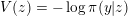 $V(z)=-\log \unicode[STIX]{x1D70B}(y|z)$
, i.e. the maximum likelihood estimator, which we assume here to be unique, for example,
$V(z)=-\log \unicode[STIX]{x1D70B}(y|z)$
, i.e. the maximum likelihood estimator, which we assume here to be unique, for example,
 $V$
is convex. In other words these homotopy methods can be used to solve optimization problems via derivative-free mean-field equations and their interacting particle approximations. See, for example, Zhang, Taghvaei and Mehta (Reference Zhang, Taghvaei and Mehta2019) and Schillings and Stuart (Reference Schillings and Stuart2017) as well as Appendices A.1 and A.3 for more details.
$V$
is convex. In other words these homotopy methods can be used to solve optimization problems via derivative-free mean-field equations and their interacting particle approximations. See, for example, Zhang, Taghvaei and Mehta (Reference Zhang, Taghvaei and Mehta2019) and Schillings and Stuart (Reference Schillings and Stuart2017) as well as Appendices A.1 and A.3 for more details.
4.2 Random data
We now replace (4.1) with an observation model of the form
 $$\begin{eqnarray}\,\text{d}Y_{t}=h(Z_{t}^{+})\,\text{d}t+\,\text{d}V_{t}^{+},\end{eqnarray}$$
where we set
 $Y_{t}\in \mathbb{R}$
for simplicity and
$Y_{t}\in \mathbb{R}$
for simplicity and
 $V_{t}^{+}$
denotes standard Brownian motion. The forward operator
$V_{t}^{+}$
denotes standard Brownian motion. The forward operator
 $h:\mathbb{R}^{N_{z}}\rightarrow \mathbb{R}$
is also assumed to be known. The marginal PDFs
$h:\mathbb{R}^{N_{z}}\rightarrow \mathbb{R}$
is also assumed to be known. The marginal PDFs
 $\widehat{\unicode[STIX]{x1D70B}}_{t}$
for
$\widehat{\unicode[STIX]{x1D70B}}_{t}$
for
 $Z_{t}$
conditioned on all observations
$Z_{t}$
conditioned on all observations
 $y_{s}$
with
$y_{s}$
with
 $s\in [0,t]$
satisfy the Kushner–Stratonovitch equation (Jazwinski Reference Jazwinski1970)
$s\in [0,t]$
satisfy the Kushner–Stratonovitch equation (Jazwinski Reference Jazwinski1970)
 $$\begin{eqnarray}\text{d}\widehat{\unicode[STIX]{x1D70B}}_{t}={\mathcal{L}}_{t}^{\dagger }\widehat{\unicode[STIX]{x1D70B}}_{t}\,\text{d}t+(h-\widehat{\unicode[STIX]{x1D70B}}_{t}[h])(\text{d}Y_{t}-\widehat{\unicode[STIX]{x1D70B}}_{t}[h]\,\text{d}t)\end{eqnarray}$$
with
 ${\mathcal{L}}^{\dagger }$
defined by (2.25). The following observation is important for the subsequent discussion.
${\mathcal{L}}^{\dagger }$
defined by (2.25). The following observation is important for the subsequent discussion.
Remark 4.4. Consider state-dependent diffusion
 $$\begin{eqnarray}\text{d}Z_{t}^{+}=\unicode[STIX]{x1D6FE}_{t}(Z_{t}^{+})\circ \,\text{d}U_{t}^{+},\end{eqnarray}$$
in its Stratonovitch interpretation (Pavliotis Reference Pavliotis2014), where
 $U_{t}^{+}$
is scalar-valued Brownian motion and
$U_{t}^{+}$
is scalar-valued Brownian motion and
 $\unicode[STIX]{x1D6FE}_{t}(z)\in \mathbb{R}^{N_{z}\times 1}$
. Here the Stratonovitch interpretation is to be applied to the implicit time-dependence of
$\unicode[STIX]{x1D6FE}_{t}(z)\in \mathbb{R}^{N_{z}\times 1}$
. Here the Stratonovitch interpretation is to be applied to the implicit time-dependence of
 $\unicode[STIX]{x1D6FE}_{t}(z)$
through
$\unicode[STIX]{x1D6FE}_{t}(z)$
through
 $Z_{t}^{+}$
only, that is, the explicit time-dependence of
$Z_{t}^{+}$
only, that is, the explicit time-dependence of
 $\unicode[STIX]{x1D6FE}_{t}$
remains to be Itô-interpreted. The associated Fokker–Planck equation for the marginal PDFs
$\unicode[STIX]{x1D6FE}_{t}$
remains to be Itô-interpreted. The associated Fokker–Planck equation for the marginal PDFs
 $\unicode[STIX]{x1D70B}_{t}$
takes the form
$\unicode[STIX]{x1D70B}_{t}$
takes the form
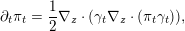 $$\begin{eqnarray}\unicode[STIX]{x2202}_{t}\unicode[STIX]{x1D70B}_{t}=\displaystyle \frac{1}{2}\unicode[STIX]{x1D6FB}_{z}\cdot (\unicode[STIX]{x1D6FE}_{t}\unicode[STIX]{x1D6FB}_{z}\cdot (\unicode[STIX]{x1D70B}_{t}\unicode[STIX]{x1D6FE}_{t})),\end{eqnarray}$$
and expectation values
 $\bar{g}=\unicode[STIX]{x1D70B}_{t}[g]$
evolve in time according to
$\bar{g}=\unicode[STIX]{x1D70B}_{t}[g]$
evolve in time according to
 $$\begin{eqnarray}\unicode[STIX]{x1D70B}_{t}[g]=\unicode[STIX]{x1D70B}_{0}[g]+\int _{0}^{t}\unicode[STIX]{x1D70B}_{s}[{\mathcal{A}}_{t}g]\,\text{d}s\end{eqnarray}$$
with operator
 ${\mathcal{A}}_{t}$
defined by
${\mathcal{A}}_{t}$
defined by
 $$\begin{eqnarray}{\mathcal{A}}_{t}g=\displaystyle \frac{1}{2}\unicode[STIX]{x1D6FE}_{t}^{\text{T}}\unicode[STIX]{x1D6FB}_{z}(\unicode[STIX]{x1D6FE}_{t}^{\text{T}}\unicode[STIX]{x1D6FB}_{z}g).\end{eqnarray}$$
Now consider the mean-field equation
 $$\begin{eqnarray}\displaystyle \frac{\text{d}}{\text{d}t}\widetilde{Z}_{t}=-\displaystyle \frac{1}{2}\unicode[STIX]{x1D6FE}_{t}(\widetilde{Z}_{t})\,J_{t},\quad J_{t}:=\widetilde{\unicode[STIX]{x1D70B}}_{t}^{-1}\unicode[STIX]{x1D6FB}_{z}\cdot (\widetilde{\unicode[STIX]{x1D70B}}_{t}\unicode[STIX]{x1D6FE}_{t}),\end{eqnarray}$$
with
 $\widetilde{\unicode[STIX]{x1D70B}}_{t}$
the law of
$\widetilde{\unicode[STIX]{x1D70B}}_{t}$
the law of
 $\widetilde{Z}_{t}$
. The associated Liouville equation is
$\widetilde{Z}_{t}$
. The associated Liouville equation is
 $$\begin{eqnarray}\unicode[STIX]{x2202}_{t}\widetilde{\unicode[STIX]{x1D70B}}_{t}=\displaystyle \frac{1}{2}\unicode[STIX]{x1D6FB}_{z}\cdot (\widetilde{\unicode[STIX]{x1D70B}}_{t}\unicode[STIX]{x1D6FE}_{t}J_{t})=\displaystyle \frac{1}{2}\unicode[STIX]{x1D6FB}_{z}\cdot (\unicode[STIX]{x1D6FE}_{t}\unicode[STIX]{x1D6FB}_{z}\cdot (\unicode[STIX]{x1D6FE}_{t}\widetilde{\unicode[STIX]{x1D70B}}_{t})).\end{eqnarray}$$
In other words, the marginal PDFs and the associated expectation values evolve identically under (4.15) and (4.18), respectively.
We now state a formulation of the continuous-time filtering problem in terms of appropriate mean-field equations. These equations follow the framework of the feedback particle filter (FPF) as first introduced by Yang et al. (Reference Yang, Mehta and Meyn2013) and theoretically justified by Laugesen et al. (Reference Laugesen, Mehta, Meyn and Raginsky2015). See Crisan and Xiong (Reference Crisan and Xiong2010) and Xiong (Reference Xiong, Crisan and Rozovskii2011) for an alternative formulation.
Lemma 4.5. The mean-field SDE
 $$\begin{eqnarray}\text{d}Z_{t}^{+}=f_{t}(Z_{t}^{+})\,\text{d}t+\unicode[STIX]{x1D6FE}^{1/2}\,\text{d}W_{t}^{+}-K_{t}(Z_{t}^{+})\circ \,\text{d}I_{t}\end{eqnarray}$$
with
 $$\begin{eqnarray}\text{d}I_{t}:=h(Z_{t}^{+})\,\text{d}t-\,\text{d}Y_{t}+\,\text{d}U_{t}^{+},\end{eqnarray}$$
 $U_{t}^{+}$
standard Brownian motion, and
$U_{t}^{+}$
standard Brownian motion, and
 $K_{t}:=\unicode[STIX]{x1D6FB}_{z}\unicode[STIX]{x1D719}_{t}$
, where the potential
$K_{t}:=\unicode[STIX]{x1D6FB}_{z}\unicode[STIX]{x1D719}_{t}$
, where the potential
 $\unicode[STIX]{x1D719}_{t}$
satisfies the elliptic PDE
$\unicode[STIX]{x1D719}_{t}$
satisfies the elliptic PDE
 $$\begin{eqnarray}\unicode[STIX]{x1D6FB}_{z}\cdot (\unicode[STIX]{x1D70B}_{t}\unicode[STIX]{x1D6FB}_{z}\unicode[STIX]{x1D719}_{t})=-\unicode[STIX]{x1D70B}_{t}(h-\unicode[STIX]{x1D70B}_{t}[h]),\end{eqnarray}$$
leads to the same evolution of its conditional marginal distributions
 $\unicode[STIX]{x1D70B}_{t}$
as (4.14).
$\unicode[STIX]{x1D70B}_{t}$
as (4.14).
Proof. We set
 $\unicode[STIX]{x1D6FE}=0$
and
$\unicode[STIX]{x1D6FE}=0$
and
 $f_{t}\equiv 0$
in (4.19) for simplicity. Then, following (4.16) with
$f_{t}\equiv 0$
in (4.19) for simplicity. Then, following (4.16) with
 $\unicode[STIX]{x1D6FE}_{t}=K_{t}$
, the Fokker–Planck equation for the marginal distributions
$\unicode[STIX]{x1D6FE}_{t}=K_{t}$
, the Fokker–Planck equation for the marginal distributions
 $\unicode[STIX]{x1D70B}_{t}$
of (4.19) conditioned on
$\unicode[STIX]{x1D70B}_{t}$
of (4.19) conditioned on
 $\{{Y_{s}\}}_{s\in [0,t]}$
is given by
$\{{Y_{s}\}}_{s\in [0,t]}$
is given by
 $$\begin{eqnarray}\displaystyle \text{d}\unicode[STIX]{x1D70B}_{t} & = & \displaystyle \unicode[STIX]{x1D6FB}_{z}\cdot (\unicode[STIX]{x1D70B}_{t}K_{t}(h(z)\,\text{d}t-\,\text{d}Y_{t}))+\unicode[STIX]{x1D6FB}_{z}\cdot (K_{t}\unicode[STIX]{x1D6FB}_{z}\cdot (\unicode[STIX]{x1D70B}_{t}K_{t}))\,\text{d}t\end{eqnarray}$$
 $$\begin{eqnarray}\displaystyle & = & \displaystyle (\unicode[STIX]{x1D70B}_{t}[h]\,\text{d}t-\,\text{d}Y_{t})\,\unicode[STIX]{x1D6FB}_{z}\cdot (\unicode[STIX]{x1D70B}_{t}K_{t})+\unicode[STIX]{x1D6FB}_{z}\cdot (\unicode[STIX]{x1D70B}_{t}K_{t}(h(z)-\unicode[STIX]{x1D70B}_{t}[h])\,\text{d}t\nonumber\\ \displaystyle & & \displaystyle \qquad +\,\unicode[STIX]{x1D6FB}_{z}\cdot (K_{t}\unicode[STIX]{x1D6FB}_{z}\cdot (\unicode[STIX]{x1D70B}_{t}K_{t}))\,\text{d}t\end{eqnarray}$$
 $$\begin{eqnarray}\displaystyle & = & \displaystyle \unicode[STIX]{x1D70B}_{t}(h-\unicode[STIX]{x1D70B}_{t}[h])(\text{d}Y_{t}-\unicode[STIX]{x1D70B}_{t}[h]\,\text{d}t),\end{eqnarray}$$
as desired, where we have used (4.20) twice to get from (4.22) to (4.23). Also note that both
 $Y_{t}$
and
$Y_{t}$
and
 $U_{t}^{+}$
contributed to the diffusion-induced final term in (4.21) and hence the factor
$U_{t}^{+}$
contributed to the diffusion-induced final term in (4.21) and hence the factor
 $1/2$
in (4.16) is replaced by one.◻
$1/2$
in (4.16) is replaced by one.◻
Remark 4.6. Using the reformulation (4.18) of (4.15) in Stratonovitch form with
 $\unicode[STIX]{x1D6FE}_{t}=K_{t}$
together with (4.20), one can replace
$\unicode[STIX]{x1D6FE}_{t}=K_{t}$
together with (4.20), one can replace
 $K_{t}\circ \text{d}U_{t}^{+}$
with
$K_{t}\circ \text{d}U_{t}^{+}$
with
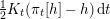 ${\textstyle \frac{1}{2}}K_{t}(\unicode[STIX]{x1D70B}_{t}[h]-h)\,\text{d}t$
, which leads to the alternative
${\textstyle \frac{1}{2}}K_{t}(\unicode[STIX]{x1D70B}_{t}[h]-h)\,\text{d}t$
, which leads to the alternative
 $$\begin{eqnarray}\,\text{d}I_{t}=\displaystyle \frac{1}{2}(h+\unicode[STIX]{x1D70B}_{t}[h])\,\text{d}t-\,\text{d}Y_{t}\end{eqnarray}$$
for the innovation
 $I_{t}$
, as originally proposed by Yang et al. (Reference Yang, Mehta and Meyn2013) in their FPF formulation. We also note that the feedback particle formulation (4.19) can be extended to systems for which the measurement and model errors are correlated. See Nüsken, Reich and Rozdeba (Reference Nüsken, Reich and Rozdeba2019) for more details.
$I_{t}$
, as originally proposed by Yang et al. (Reference Yang, Mehta and Meyn2013) in their FPF formulation. We also note that the feedback particle formulation (4.19) can be extended to systems for which the measurement and model errors are correlated. See Nüsken, Reich and Rozdeba (Reference Nüsken, Reich and Rozdeba2019) for more details.
The ensemble Kalman–Bucy filter (Bergemann and Reich Reference Bergemann and Reich2012) with the Kalman gain factor
 $K_{t}$
being independent of the state variable
$K_{t}$
being independent of the state variable
 $z$
and of the form
$z$
and of the form
 $$\begin{eqnarray}K_{t}=P_{t}^{zh}\end{eqnarray}$$
can be viewed as a special case of an FPF. Here
 $P_{t}^{zh}$
denotes the covariance matrix between
$P_{t}^{zh}$
denotes the covariance matrix between
 $Z_{t}$
and
$Z_{t}$
and
 $h(Z_{t})$
at time
$h(Z_{t})$
at time
 $t$
.
$t$
.
5 Numerical methods
In this section we discuss some numerical implementations of the mean-field approach to continuous-time data assimilation. An introduction to standard particle filter implementations can, for example, be found in Bain and Crisan (Reference Bain and Crisan2008). We start with the continuous-time formulation of the ensemble Kalman filter and state a numerical implementation of the FPF using a Schrödinger formulation in the second part of this section. See also Appendix A.1 for some more details on a particle-based solution of the elliptic PDEs (4.4), (4.13) and (4.20), respectively.
5.1 Ensemble Kalman–Bucy filter
Let us start with the ensemble Kalman–Bucy filter (EnKBF), which arises naturally from the mean-field equations (4.7) and (4.19), respectively, with Kalman gain (4.24) (Bergemann and Reich Reference Bergemann and Reich2012). We state the EnKBF here in the form
 $$\begin{eqnarray}\text{d}Z_{t}^{i}=f_{t}(Z_{t}^{i})\,\text{d}t+\unicode[STIX]{x1D6FE}^{1/2}\,\text{d}W_{t}^{+}-K_{t}^{M}\,\text{d}I_{t}^{i}\end{eqnarray}$$
for
 $i=1,\ldots ,M$
and
$i=1,\ldots ,M$
and
 $$\begin{eqnarray}K_{t}^{M}:=\displaystyle \frac{1}{M-1}\mathop{\sum }_{i=1}^{M}Z_{t}^{i}(h(Z_{t}^{i})-\bar{h}_{t}^{M})^{\text{T}},\quad \bar{h}_{t}^{M}:=\displaystyle \frac{1}{M}\mathop{\sum }_{i=1}^{M}h(Z_{t}^{i}).\end{eqnarray}$$
The innovations
 $\text{d}I_{t}^{i}$
take different forms depending on whether the data are smooth in time, that is,
$\text{d}I_{t}^{i}$
take different forms depending on whether the data are smooth in time, that is,
 $$\begin{eqnarray}\text{d}I_{t}^{i}=\displaystyle \frac{1}{2}(h(Z_{t}^{i})+\bar{h}_{t}^{M}-2y_{t})\,\text{d}t,\end{eqnarray}$$
or contains stochastic contributions, that is,
 $$\begin{eqnarray}\text{d}I_{t}^{i}=\displaystyle \frac{1}{2}(h(Z_{t}^{i})+\bar{h}_{t}^{M})\,\text{d}t-\,\text{d}y_{t},\end{eqnarray}$$
or, alternatively,
 $$\begin{eqnarray}\text{d}I_{t}^{i}=h(Z_{t}^{i})\,\text{d}t+\,\text{d}U_{t}^{i}-\,\text{d}y_{t},\end{eqnarray}$$
where
 $U_{t}^{i}$
denotes standard Brownian motion. The SDEs (5.1) can be discretized in time by any suitable time-stepping method such as the Euler–Maruyama scheme (Kloeden and Platen Reference Kloeden and Platen1992). However, one has to be careful with the choice of the step-size
$U_{t}^{i}$
denotes standard Brownian motion. The SDEs (5.1) can be discretized in time by any suitable time-stepping method such as the Euler–Maruyama scheme (Kloeden and Platen Reference Kloeden and Platen1992). However, one has to be careful with the choice of the step-size
 $\unicode[STIX]{x1D6E5}t$
due to potentially stiff contributions from
$\unicode[STIX]{x1D6E5}t$
due to potentially stiff contributions from
 $K_{t}^{M}\,\text{d}I_{t}^{i}$
. See, for example, Amezcua, Kalnay, Ide and Reich (Reference Amezcua, Kalnay, Ide and Reich2014) and Blömker, Schillings and Wacker (Reference Blömker, Schillings and Wacker2018).
$K_{t}^{M}\,\text{d}I_{t}^{i}$
. See, for example, Amezcua, Kalnay, Ide and Reich (Reference Amezcua, Kalnay, Ide and Reich2014) and Blömker, Schillings and Wacker (Reference Blömker, Schillings and Wacker2018).
Remark 5.1. It is of broad interest to study the stability and accuracy of interacting particle filter algorithms such as the discrete-time EnKF and the continuous-time EnKBF for fixed particle numbers
 $M$
. On the negative side, it has been shown by Kelly, Majda and Tong (Reference Kelly, Majda and Tong2015) that such algorithms can undergo finite-time instabilities, while it has also been demonstrated (González-Tokman and Hunt Reference González-Tokman and Hunt2013, Kelly, Law and Stuart Reference Kelly, Law and Stuart2014, Tong, Majda and Kelly Reference Tong, Majda and Kelly2016, de Wiljes, Reich and Stannat Reference de Wiljes, Reich and Stannat2018) that such algorithms can be stable and accurate under appropriate conditions on the dynamics and measurement process. Asymptotic properties of the EnKF and EnKBF in the limit of
$M$
. On the negative side, it has been shown by Kelly, Majda and Tong (Reference Kelly, Majda and Tong2015) that such algorithms can undergo finite-time instabilities, while it has also been demonstrated (González-Tokman and Hunt Reference González-Tokman and Hunt2013, Kelly, Law and Stuart Reference Kelly, Law and Stuart2014, Tong, Majda and Kelly Reference Tong, Majda and Kelly2016, de Wiljes, Reich and Stannat Reference de Wiljes, Reich and Stannat2018) that such algorithms can be stable and accurate under appropriate conditions on the dynamics and measurement process. Asymptotic properties of the EnKF and EnKBF in the limit of
 $M\rightarrow \infty$
have also been studied, for example, by Le Gland, Monbet and Tran (Reference Le Gland, Monbet, Tran, Crisan and Rozovskii2011), Kwiatowski and Mandel (Reference Kwiatowski and Mandel2015) and de Wiljes et al. (Reference de Wiljes, Reich and Stannat2018).
$M\rightarrow \infty$
have also been studied, for example, by Le Gland, Monbet and Tran (Reference Le Gland, Monbet, Tran, Crisan and Rozovskii2011), Kwiatowski and Mandel (Reference Kwiatowski and Mandel2015) and de Wiljes et al. (Reference de Wiljes, Reich and Stannat2018).
5.2 Feedback particle filter
A Monte Carlo implementation of the FPF (4.19) faces two main obstacles. First, one needs to approximate the potential
 $\unicode[STIX]{x1D719}_{t}$
in (4.20) with the density
$\unicode[STIX]{x1D719}_{t}$
in (4.20) with the density
 $\unicode[STIX]{x1D70B}_{t}$
, which is only available in terms of an empirical measure
$\unicode[STIX]{x1D70B}_{t}$
, which is only available in terms of an empirical measure
 $$\begin{eqnarray}\unicode[STIX]{x1D70B}_{t}(z)=\displaystyle \frac{1}{M}\mathop{\sum }_{i=1}^{M}\unicode[STIX]{x1D6FF}(z-z_{t}^{i}).\end{eqnarray}$$
Several possible approximations have been discussed by Taghvaei and Mehta (Reference Taghvaei and Mehta2016) and Taghvaei, de Wiljes, Mehta and Reich (Reference Taghvaei, de Wiljes, Mehta and Reich2017). Here we would like to mention in particular an approximation based on diffusion maps, which we summarize in Appendix A.1. Second, one needs to apply suitable time-stepping methods for the SDE (4.19) in Stratonovitch form. Here we suggest using the Euler–Heun method (Burrage, Burrage and Tian Reference Burrage, Burrage and Tian2004),
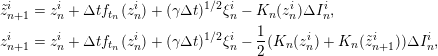 $$\begin{eqnarray}\displaystyle \tilde{z}_{n+1}^{i} & = & \displaystyle z_{n}^{i}+\unicode[STIX]{x1D6E5}tf_{t_{n}}(z_{n}^{i})+(\unicode[STIX]{x1D6FE}\unicode[STIX]{x1D6E5}t)^{1/2}\unicode[STIX]{x1D709}_{n}^{i}-K_{n}(z_{n}^{i})\unicode[STIX]{x1D6E5}I_{n}^{i},\nonumber\\ \displaystyle z_{n+1}^{i} & = & \displaystyle z_{n}^{i}+\unicode[STIX]{x1D6E5}tf_{t_{n}}(z_{n}^{i})+(\unicode[STIX]{x1D6FE}\unicode[STIX]{x1D6E5}t)^{1/2}\unicode[STIX]{x1D709}_{n}^{i}-\displaystyle \frac{1}{2}(K_{n}(z_{n}^{i})+K_{n}(\tilde{z}_{n+1}^{i}))\unicode[STIX]{x1D6E5}I_{n}^{i},\nonumber\end{eqnarray}$$
 $i=1,\ldots ,M$
, with, for example,
$i=1,\ldots ,M$
, with, for example,
 $$\begin{eqnarray}\unicode[STIX]{x1D6E5}I_{n}^{i}=\displaystyle \frac{1}{2}(h(z_{n}^{i})+\bar{h}_{n}^{M})\unicode[STIX]{x1D6E5}t-\unicode[STIX]{x1D6E5}y_{n}.\end{eqnarray}$$
While the above implementation of the FPF requires one to solve the elliptic PDE (4.20) twice per time-step, we now suggest a time-stepping approach in terms of an associated Schrödinger problem. Let us assume that we have
 $M$
equally weighted particles
$M$
equally weighted particles
 $z_{n}^{i}$
representing the conditional filtering distribution at time
$z_{n}^{i}$
representing the conditional filtering distribution at time
 $t_{n}$
. We first propagate these particles forward under the drift term alone, that is,
$t_{n}$
. We first propagate these particles forward under the drift term alone, that is,
 $$\begin{eqnarray}\hat{z}_{n+1}^{i}:=z_{n}^{i}+\unicode[STIX]{x1D6E5}t\,f_{t_{n}}(z_{n}^{i}),\quad i=1,\ldots ,M.\end{eqnarray}$$
In the next step, we draw
 $L=KM$
with
$L=KM$
with
 $K\geq 1$
samples
$K\geq 1$
samples
 $\widetilde{z}_{n+1}^{l}$
from the forecast PDF
$\widetilde{z}_{n+1}^{l}$
from the forecast PDF
 $$\begin{eqnarray}\widetilde{\unicode[STIX]{x1D70B}}(z):=\displaystyle \frac{1}{M}\mathop{\sum }_{i=1}^{M}\text{n}(z;\hat{z}_{n+1}^{i},\unicode[STIX]{x1D6FE}\unicode[STIX]{x1D6E5}tI)\end{eqnarray}$$
and assign importance weights
 $$\begin{eqnarray}w_{n+1}^{l}\propto \exp \biggl(-\displaystyle \frac{\unicode[STIX]{x1D6E5}t}{2}(h(\widetilde{z}_{n+1}^{l}))^{2}+\unicode[STIX]{x1D6E5}y_{n}h(\widetilde{z}_{n+1}^{l})\biggr)\end{eqnarray}$$
with normalization (3.24). Recall that we assumed that
 $y_{t}\in \mathbb{R}$
for simplicity and
$y_{t}\in \mathbb{R}$
for simplicity and
 $\unicode[STIX]{x1D6E5}y_{n}:=y_{t_{n+1}}-y_{t_{n}}$
. We then solve the Schrödinger problem
$\unicode[STIX]{x1D6E5}y_{n}:=y_{t_{n+1}}-y_{t_{n}}$
. We then solve the Schrödinger problem
 $$\begin{eqnarray}P^{\ast }=\arg \min _{P\in \unicode[STIX]{x1D6F1}_{\text{M}}}\text{KL}(P||Q)\end{eqnarray}$$
with the entries of
 $Q\in \mathbb{R}^{L\times M}$
given by
$Q\in \mathbb{R}^{L\times M}$
given by
 $$\begin{eqnarray}q_{li}=\exp \biggl(-\displaystyle \frac{1}{2\unicode[STIX]{x1D6FE}\unicode[STIX]{x1D6E5}t}\Vert \widetilde{z}_{n+1}^{l}-\hat{z}_{n+1}^{i}\Vert ^{2}\biggr)\end{eqnarray}$$
and the set
 $\unicode[STIX]{x1D6F1}_{\text{M}}$
defined by (3.26). The desired particles
$\unicode[STIX]{x1D6F1}_{\text{M}}$
defined by (3.26). The desired particles
 $z_{n+1}^{i}=Z_{n+1}^{i}(\unicode[STIX]{x1D714})$
are finally given as realizations of
$z_{n+1}^{i}=Z_{n+1}^{i}(\unicode[STIX]{x1D714})$
are finally given as realizations of
 $$\begin{eqnarray}Z_{n+1}^{i}=\mathop{\sum }_{l=1}^{L}\widetilde{z}_{n+1}^{l}p_{li}^{\ast }+(\unicode[STIX]{x1D6FE}\unicode[STIX]{x1D6E5}t)^{1/2}\unicode[STIX]{x1D6EF}_{n}^{i},\quad \unicode[STIX]{x1D6EF}_{n}^{i}\sim \text{N}(0,I),\end{eqnarray}$$
for
 $i=1,\ldots ,M$
.
$i=1,\ldots ,M$
.
The update (5.4), with
 $P^{\ast }$
defined by (5.3), can be viewed as data-driven drift correction combined with a standard approximation to the Brownian diffusion part of the underlying SDE model. It remains to be investigated in what sense (5.4) can be viewed as an approximation to the FPF formulation (4.19) as
$P^{\ast }$
defined by (5.3), can be viewed as data-driven drift correction combined with a standard approximation to the Brownian diffusion part of the underlying SDE model. It remains to be investigated in what sense (5.4) can be viewed as an approximation to the FPF formulation (4.19) as
 $M\rightarrow \infty$
and
$M\rightarrow \infty$
and
 $\unicode[STIX]{x1D6E5}t\rightarrow 0$
.
$\unicode[STIX]{x1D6E5}t\rightarrow 0$
.
Remark 5.2. One can also use the matrix
 $P^{\ast }$
from (5.3) to implement a resampling scheme
$P^{\ast }$
from (5.3) to implement a resampling scheme
 $$\begin{eqnarray}\mathbb{P}[Z_{n+1}^{i}(\unicode[STIX]{x1D714})=\widetilde{z}_{n+1}^{l}]=p_{li}^{\ast }\end{eqnarray}$$
for
 $i=1,\ldots ,M$
. Note that, contrary to classical resampling schemes based on weighted particles
$i=1,\ldots ,M$
. Note that, contrary to classical resampling schemes based on weighted particles
 $(\widetilde{z}_{n+1}^{l},w_{n+1}^{l})$
,
$(\widetilde{z}_{n+1}^{l},w_{n+1}^{l})$
,
 $l=1,\ldots ,L$
, the sampling probabilities
$l=1,\ldots ,L$
, the sampling probabilities
 $p_{li}^{\ast }$
take into account the underlying geometry of the forecasts
$p_{li}^{\ast }$
take into account the underlying geometry of the forecasts
 $\hat{z}_{n+1}^{i}$
in state space.
$\hat{z}_{n+1}^{i}$
in state space.
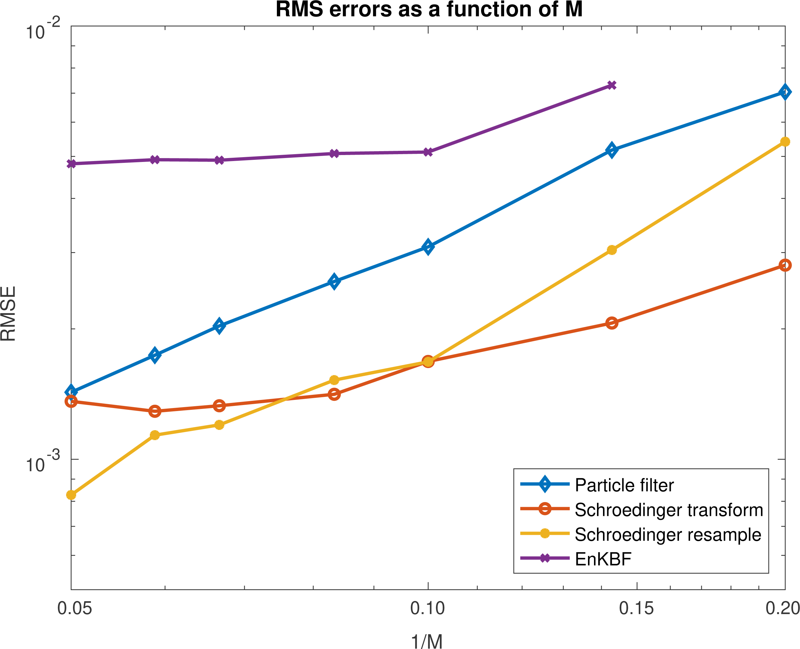
Figure 5.1. RMS errors as a function of sample size,
 $M$
, for a standard particle filter, the EnKBF, and implementations of (5.4) (Schrödinger transform) and (5.5) (Schrödinger resample), respectively. Both Schrödinger-based methods outperform the standard particle filter for small ensemble sizes. The EnKBF diverged for the smallest ensemble size of
$M$
, for a standard particle filter, the EnKBF, and implementations of (5.4) (Schrödinger transform) and (5.5) (Schrödinger resample), respectively. Both Schrödinger-based methods outperform the standard particle filter for small ensemble sizes. The EnKBF diverged for the smallest ensemble size of
 $M=5$
and performed worse than all other methods for this highly nonlinear problem.
$M=5$
and performed worse than all other methods for this highly nonlinear problem.
Example 5.3. We consider the SDE formulation
 $$\begin{eqnarray}\text{d}Z_{t}=f(Z_{t})\,\text{d}t+\unicode[STIX]{x1D6FE}^{1/2}\,\text{d}W_{t}\end{eqnarray}$$
of a stochastically perturbed Lorenz-63 model (Lorenz Reference Lorenz1963, Reich and Cotter Reference Reich and Cotter2015, Law et al.
Reference Law, Stuart and Zygalakis2015) with diffusion constant
 $\unicode[STIX]{x1D6FE}=0.1$
. The system is fully observed according to
$\unicode[STIX]{x1D6FE}=0.1$
. The system is fully observed according to
 $$\begin{eqnarray}\text{d}Y_{t}=f(Z_{t})\,\text{d}t+R^{1/2}\,\text{d}V_{t}\end{eqnarray}$$
with measurement error variance
 $R=0.1$
, and the system is simulated over a time interval
$R=0.1$
, and the system is simulated over a time interval
 $t\in [0,40\,000]$
with step-size
$t\in [0,40\,000]$
with step-size
 $\unicode[STIX]{x1D6E5}t=0.01$
. We implemented a standard particle filter with resampling performed after each time-step and compared the resulting RMS errors with those arising from using (5.4) (Schrödinger transform) and (5.5) (Schrödinger resample), respectively. See Figure 5.1. It can be seen that the Schrödinger-based methods outperform the standard particle filter in terms of RMS errors for small ensemble sizes. The Schrödinger transform method is particularly robust for very small ensemble sizes while Schrödinger resample performs better at larger sample sizes. We also implemented the EnKBF (5.1) and found that it diverged for the smallest ensemble size of
$\unicode[STIX]{x1D6E5}t=0.01$
. We implemented a standard particle filter with resampling performed after each time-step and compared the resulting RMS errors with those arising from using (5.4) (Schrödinger transform) and (5.5) (Schrödinger resample), respectively. See Figure 5.1. It can be seen that the Schrödinger-based methods outperform the standard particle filter in terms of RMS errors for small ensemble sizes. The Schrödinger transform method is particularly robust for very small ensemble sizes while Schrödinger resample performs better at larger sample sizes. We also implemented the EnKBF (5.1) and found that it diverged for the smallest ensemble size of
 $M=5$
and performed worse than the other methods for larger ensemble sizes.
$M=5$
and performed worse than the other methods for larger ensemble sizes.
6 Conclusions
We have summarized sequential data assimilation techniques suitable for state estimation of discrete- and continuous-time stochastic processes. In addition to algorithmic approaches based on the standard filtering and smoothing framework of stochastic analysis, we have drawn a connection to a boundary value problem over joint probability measures first formulated by Erwin Schrödinger. We have argued that sequential data assimilation essentially needs to approximate such a boundary value problem with the boundary conditions given by the filtering distributions at consecutive observation times.
Application of these techniques to high-dimensional problems arising, for example, from the spatial discretization of PDEs requires further approximations in the form of localization and inflation, which we have not discussed in this survey. See, for example, Evensen (Reference Evensen2006), Reich and Cotter (Reference Reich and Cotter2015) and Asch et al. (Reference Asch, Bocquet and Nodet2017) for further details. In particular, the localization framework for particle filters as introduced by Chen and Reich (Reference Chen, Reich and van Leeuwen2015) and Reich and Cotter (Reference Reich and Cotter2015) in the context of scenario (A) could be generalized to scenarios (B) and (C) from Definition 2.4.
Finally, the approaches and computational techniques discussed in this paper are also relevant to combined state and parameter estimation.
Acknowledgement
This research has been partially funded by Deutsche Forschungsgemeinschaft (DFG) through grant CRC 1294 ‘Data Assimilation’. Feedback on earlier versions of this paper by Nikolas Kantas, Prashant Mehta and Tim Sullivan has been invaluable.
Appendices
A.1 Mesh-free approximations to Fokker–Planck and backward Kolmogorov equations
In this appendix we discuss two closely related approximations, first to the Fokker–Planck equation (2.26) with the (time-independent) operator (2.25) taking the special form
 $$\begin{eqnarray}{\mathcal{L}}^{\dagger }\unicode[STIX]{x1D70B}=-\unicode[STIX]{x1D6FB}_{z}\cdot (\unicode[STIX]{x1D70B}\,\unicode[STIX]{x1D6FB}_{z}\log \unicode[STIX]{x1D70B}^{\ast })+\unicode[STIX]{x1D6E5}_{z}\unicode[STIX]{x1D70B}=\unicode[STIX]{x1D6FB}_{z}\cdot \biggl(\unicode[STIX]{x1D70B}^{\ast }\unicode[STIX]{x1D6FB}_{z}\displaystyle \frac{\unicode[STIX]{x1D70B}}{\unicode[STIX]{x1D70B}^{\ast }}\biggr)\end{eqnarray}$$
and, second, to its adjoint operator
 ${\mathcal{L}}$
given by (3.10).
${\mathcal{L}}$
given by (3.10).
The approximation to the Fokker–Planck equation (2.26) with drift term
 $$\begin{eqnarray}f_{t}(z)=\unicode[STIX]{x1D6FB}_{z}\log \unicode[STIX]{x1D70B}^{\ast }(z)\end{eqnarray}$$
can be used to transform samples
 $x_{0}^{i}$
,
$x_{0}^{i}$
,
 $i=1,\ldots ,M$
from a (prior) PDF
$i=1,\ldots ,M$
from a (prior) PDF
 $\unicode[STIX]{x1D70B}_{0}$
into samples from a target (posterior) PDF
$\unicode[STIX]{x1D70B}_{0}$
into samples from a target (posterior) PDF
 $\unicode[STIX]{x1D70B}^{\ast }$
using an evolution equation of the form
$\unicode[STIX]{x1D70B}^{\ast }$
using an evolution equation of the form
 $$\begin{eqnarray}\displaystyle \frac{\text{d}}{\text{d}s}\breve{Z}_{s}=F_{s}(\breve{Z}_{s}),\end{eqnarray}$$
with
 $\breve{Z}_{0}\sim \breve{\unicode[STIX]{x1D70B}}_{0}:=\unicode[STIX]{x1D70B}_{0}$
such that
$\breve{Z}_{0}\sim \breve{\unicode[STIX]{x1D70B}}_{0}:=\unicode[STIX]{x1D70B}_{0}$
such that
 $$\begin{eqnarray}\lim _{s\rightarrow \infty }\breve{Z}_{s}\sim \unicode[STIX]{x1D70B}^{\ast }.\end{eqnarray}$$
The evolution of the marginal PDFs
 $\breve{\unicode[STIX]{x1D70B}}_{s}$
is given by Liouville’s equation
$\breve{\unicode[STIX]{x1D70B}}_{s}$
is given by Liouville’s equation
 $$\begin{eqnarray}\unicode[STIX]{x2202}_{s}\breve{\unicode[STIX]{x1D70B}}_{s}=-\unicode[STIX]{x1D6FB}_{z}\cdot (\breve{\unicode[STIX]{x1D70B}}_{s}F_{s}).\end{eqnarray}$$
We now choose
 $F_{s}$
such that the Kullback–Leibler divergence
$F_{s}$
such that the Kullback–Leibler divergence
 $\text{KL}\,(\breve{\unicode[STIX]{x1D70B}}_{s}||\unicode[STIX]{x1D70B}^{\ast })$
is non-increasing in time, that is,
$\text{KL}\,(\breve{\unicode[STIX]{x1D70B}}_{s}||\unicode[STIX]{x1D70B}^{\ast })$
is non-increasing in time, that is,
 $$\begin{eqnarray}\displaystyle \frac{\text{d}}{\text{d}s}\text{KL}\,(\breve{\unicode[STIX]{x1D70B}}_{s}||\unicode[STIX]{x1D70B}^{\ast })=\int \breve{\unicode[STIX]{x1D70B}}_{s}\bigg\{F_{s}\cdot \unicode[STIX]{x1D6FB}_{z}\log \displaystyle \frac{\breve{\unicode[STIX]{x1D70B}}_{s}}{\unicode[STIX]{x1D70B}^{\ast }}\bigg\}\,\text{d}z\leq 0.\end{eqnarray}$$
A natural choice is
 $$\begin{eqnarray}F_{s}(z):=-\unicode[STIX]{x1D6FB}_{z}\log \displaystyle \frac{\breve{\unicode[STIX]{x1D70B}}_{s}}{\unicode[STIX]{x1D70B}^{\ast }}(z),\end{eqnarray}$$
which renders (A.3) formally equivalent to the Fokker–Planck equation (2.26) with drift term (A.1) (Reich and Cotter Reference Reich and Cotter2015, Peyre and Cuturi Reference Peyre and Cuturi2018).
Let us now approximate the evolution equation (A.2) over a reproducing kernel Hilbert space (RKHS)
 ${\mathcal{H}}$
with kernel
${\mathcal{H}}$
with kernel
 $k(z-z^{\prime })$
and inner product
$k(z-z^{\prime })$
and inner product
 $\langle f,g\rangle _{{\mathcal{H}}}$
, which satisfies the reproducing property
$\langle f,g\rangle _{{\mathcal{H}}}$
, which satisfies the reproducing property
 $$\begin{eqnarray}\langle k(\cdot -z^{\prime }),f\rangle _{{\mathcal{H}}}=f(z^{\prime }).\end{eqnarray}$$
Following Russo (Reference Russo1990) and Degond and Mustieles (Reference Degond and Mustieles1990), we first introduce the approximation
 $$\begin{eqnarray}\widetilde{\unicode[STIX]{x1D70B}}_{s}(z):=\displaystyle \frac{1}{M}\mathop{\sum }_{i=1}^{M}k(z-z_{s}^{i})\end{eqnarray}$$
to the marginal densities
 $\breve{\unicode[STIX]{x1D70B}}_{s}$
. Note that (A.5) implies that
$\breve{\unicode[STIX]{x1D70B}}_{s}$
. Note that (A.5) implies that
 $$\begin{eqnarray}\langle f,\widetilde{\unicode[STIX]{x1D70B}}_{s}\rangle _{{\mathcal{H}}}=\displaystyle \frac{1}{M}\mathop{\sum }_{i=1}^{M}f(z_{s}^{i}).\end{eqnarray}$$
Given some evolution equations
 $$\begin{eqnarray}\displaystyle \frac{\text{d}}{\text{d}s}z_{s}^{i}=u_{s}^{i}\end{eqnarray}$$
for the particles
 $z_{s}^{i}$
,
$z_{s}^{i}$
,
 $i=1,\ldots ,M$
, we find that (A.6) satisfies Liouville’s equation, that is,
$i=1,\ldots ,M$
, we find that (A.6) satisfies Liouville’s equation, that is,
 $$\begin{eqnarray}\unicode[STIX]{x2202}_{s}\widetilde{\unicode[STIX]{x1D70B}}_{s}=-\unicode[STIX]{x1D6FB}_{z}\cdot (\widetilde{\unicode[STIX]{x1D70B}}_{s}\widetilde{F}_{s})\end{eqnarray}$$
with
 $$\begin{eqnarray}\widetilde{F}_{s}(z)=\displaystyle \frac{\mathop{\sum }_{i=1}^{M}k(z-z_{s}^{i})\,u_{s}^{i}}{\mathop{\sum }_{i=1}^{M}k(z-z_{s}^{i})}.\end{eqnarray}$$
We finally introduce the functional
 $$\begin{eqnarray}{\mathcal{V}}(\{z_{s}^{l}\}):=\langle \widetilde{\unicode[STIX]{x1D70B}}_{s},\log \displaystyle \frac{\widetilde{\unicode[STIX]{x1D70B}}_{s}}{\unicode[STIX]{x1D70B}^{\ast }}\rangle _{{\mathcal{H}}}=\displaystyle \frac{1}{M}\mathop{\sum }_{i=1}^{M}\log \displaystyle \frac{{\textstyle \frac{1}{M}}\mathop{\sum }_{j=1}^{M}k(z_{s}^{i}-z_{s}^{j})}{\unicode[STIX]{x1D70B}^{\ast }(z_{s}^{i})}\end{eqnarray}$$
as an approximation to the Kullback–Leibler divergence in the RKHS
 ${\mathcal{H}}$
and set
${\mathcal{H}}$
and set
 $$\begin{eqnarray}u_{s}^{i}:=-M\unicode[STIX]{x1D6FB}_{z_{s}^{i}}{\mathcal{V}}(\{z_{s}^{l}\}),\end{eqnarray}$$
which constitutes the desired particle approximation to the Fokker–Planck equation (2.26) with drift term (A.1). Time-stepping methods for such gradient flow systems have been discussed by Pathiraja and Reich (Reference Pathiraja and Reich2019).
We also remark that an alternative interacting particle system, approximating the same asymptotic PDF
 $\unicode[STIX]{x1D70B}^{\ast }$
in the limit
$\unicode[STIX]{x1D70B}^{\ast }$
in the limit
 $s\rightarrow \infty$
, has been proposed recently by Liu and Wang (Reference Liu, Wang and Lee2016) under the notion of Stein variational descent. See Lu, Lu and Nolen (Reference Lu, Lu and Nolen2019) for a theoretical analysis of Stein variational descent, which implies in particular that Stein variational descent can be viewed as a Lagrangian particle approximation to the modified evolution equation
$s\rightarrow \infty$
, has been proposed recently by Liu and Wang (Reference Liu, Wang and Lee2016) under the notion of Stein variational descent. See Lu, Lu and Nolen (Reference Lu, Lu and Nolen2019) for a theoretical analysis of Stein variational descent, which implies in particular that Stein variational descent can be viewed as a Lagrangian particle approximation to the modified evolution equation
 $$\begin{eqnarray}\unicode[STIX]{x2202}_{s}\breve{\unicode[STIX]{x1D70B}}_{s}=\unicode[STIX]{x1D6FB}_{z}\cdot \biggl(\breve{\unicode[STIX]{x1D70B}}_{s}^{2}\unicode[STIX]{x1D6FB}_{z}\log \displaystyle \frac{\breve{\unicode[STIX]{x1D70B}}_{s}}{\unicode[STIX]{x1D70B}^{\ast }}(z)\biggr)=\unicode[STIX]{x1D6FB}_{z}\cdot (\breve{\unicode[STIX]{x1D70B}}_{s}(\unicode[STIX]{x1D6FB}_{z}\breve{\unicode[STIX]{x1D70B}}_{s}-\breve{\unicode[STIX]{x1D70B}}_{s}\unicode[STIX]{x1D6FB}_{z}\log \unicode[STIX]{x1D70B}^{\ast }))\end{eqnarray}$$
in the marginal PDFs
 $\breve{\unicode[STIX]{x1D70B}}_{s}$
, that is, one uses
$\breve{\unicode[STIX]{x1D70B}}_{s}$
, that is, one uses
 $$\begin{eqnarray}F_{s}(z):=-\breve{\unicode[STIX]{x1D70B}}_{s}\unicode[STIX]{x1D6FB}_{z}\log \displaystyle \frac{\breve{\unicode[STIX]{x1D70B}}_{s}}{\unicode[STIX]{x1D70B}^{\ast }}(z)\end{eqnarray}$$
in (A.2). The Kullback–Leibler divergence is still non-increasing since (A.4) becomes
 $$\begin{eqnarray}\displaystyle \frac{\text{d}}{\text{d}s}\text{KL}\,(\breve{\unicode[STIX]{x1D70B}}_{s}||\unicode[STIX]{x1D70B}^{\ast })=-\int \Vert F_{s}\Vert ^{2}\,\text{d}z\leq 0.\end{eqnarray}$$
A numerical discretization is obtained through the approximation
 $$\begin{eqnarray}F_{s}(z^{\prime })\approx \int F_{s}(z)\,k(z-z^{\prime })\,\text{d}z,\end{eqnarray}$$
that is, one views the kernel
 $k(z-z^{\prime })$
as a regularized Dirac delta function. This approximation leads to another vector field
$k(z-z^{\prime })$
as a regularized Dirac delta function. This approximation leads to another vector field
 $$\begin{eqnarray}\displaystyle \widehat{F}_{s}(z^{\prime }) & := & \displaystyle -\int \breve{\unicode[STIX]{x1D70B}}_{s}(z)\{\unicode[STIX]{x1D6FB}_{z}\log \breve{\unicode[STIX]{x1D70B}}_{s}(z)-\unicode[STIX]{x1D6FB}_{z}\log \unicode[STIX]{x1D70B}^{\ast }(z)\}k(z-z^{\prime })\,\text{d}z\nonumber\\ \displaystyle & = & \displaystyle \int \breve{\unicode[STIX]{x1D70B}}_{s}(z)\{\unicode[STIX]{x1D6FB}_{z}k(z-z^{\prime })+k(z-z^{\prime })\,\unicode[STIX]{x1D6FB}_{z}\log \unicode[STIX]{x1D70B}^{\ast }(z)\}\,\text{d}z.\nonumber\end{eqnarray}$$
On extending the RKHS
 ${\mathcal{H}}$
and its reproducing property (A.5) component-wise to vector-valued functions, it follows that
${\mathcal{H}}$
and its reproducing property (A.5) component-wise to vector-valued functions, it follows that
 $$\begin{eqnarray}\frac{\text{d}}{\text{d}s}\text{KL}\,(\breve{\unicode[STIX]{x1D70B}}_{s}||\unicode[STIX]{x1D70B}^{\ast })=-\int F_{s}\cdot \widehat{F}_{s}\,\text{d}z=-\langle \widehat{F}_{s},\widehat{F}_{s}\rangle _{{\mathcal{H}}}\leq 0\end{eqnarray}$$
along transformations induced by the vector field
 $\widehat{F}_{s}$
. See Liu and Wang (Reference Liu, Wang and Lee2016) for more details.
$\widehat{F}_{s}$
. See Liu and Wang (Reference Liu, Wang and Lee2016) for more details.
We now turn our attention to the dual operator
 ${\mathcal{L}}_{t}$
, defined by (3.10), which also arises from (4.6) and (4.20), respectively. More specifically, let us rewrite (4.20) in the form
${\mathcal{L}}_{t}$
, defined by (3.10), which also arises from (4.6) and (4.20), respectively. More specifically, let us rewrite (4.20) in the form
 $$\begin{eqnarray}{\mathcal{A}}_{t}\unicode[STIX]{x1D719}_{t}=-(h-\unicode[STIX]{x1D70B}_{t}[h])\end{eqnarray}$$
with the operator
 ${\mathcal{A}}_{t}$
defined by
${\mathcal{A}}_{t}$
defined by
 $$\begin{eqnarray}{\mathcal{A}}_{t}g:=\displaystyle \frac{1}{\unicode[STIX]{x1D70B}_{t}}\unicode[STIX]{x1D6FB}_{z}\cdot (\unicode[STIX]{x1D70B}_{t}\unicode[STIX]{x1D6FB}_{z}g).\end{eqnarray}$$
Then we find that
 ${\mathcal{A}}_{t}$
is of the form of
${\mathcal{A}}_{t}$
is of the form of
 ${\mathcal{L}}_{t}$
with
${\mathcal{L}}_{t}$
with
 $\unicode[STIX]{x1D70B}_{t}$
taking the role of
$\unicode[STIX]{x1D70B}_{t}$
taking the role of
 $\unicode[STIX]{x1D70B}^{\ast }$
.
$\unicode[STIX]{x1D70B}^{\ast }$
.
We also recall that (3.11) provides an approximation to
 ${\mathcal{L}}_{t}$
and hence to
${\mathcal{L}}_{t}$
and hence to
 ${\mathcal{A}}_{t}$
. This observation allows one to introduce a sample-based method for approximating the potential
${\mathcal{A}}_{t}$
. This observation allows one to introduce a sample-based method for approximating the potential
 $\unicode[STIX]{x1D719}$
defined by the elliptic partial differential equation (A.8) for a given function
$\unicode[STIX]{x1D719}$
defined by the elliptic partial differential equation (A.8) for a given function
 $h(z)$
.
$h(z)$
.
Here we instead follow the presentation of Taghvaei and Mehta (Reference Taghvaei and Mehta2016) and Taghvaei et al. (Reference Taghvaei, de Wiljes, Mehta and Reich2017) and assume that we have
 $M$
samples
$M$
samples
 $z^{i}$
from a PDF
$z^{i}$
from a PDF
 $\unicode[STIX]{x1D70B}$
. The method is based on
$\unicode[STIX]{x1D70B}$
. The method is based on
 $$\begin{eqnarray}\displaystyle \frac{\unicode[STIX]{x1D719}-\text{e}^{\unicode[STIX]{x1D716}{\mathcal{A}}}\unicode[STIX]{x1D719}}{\unicode[STIX]{x1D716}}\approx h-\unicode[STIX]{x1D70B}[h]\end{eqnarray}$$
for
 $\unicode[STIX]{x1D716}>0$
sufficiently small and upon replacing
$\unicode[STIX]{x1D716}>0$
sufficiently small and upon replacing
 $\text{e}^{\unicode[STIX]{x1D716}{\mathcal{A}}}$
with a diffusion map approximation (Harlim Reference Harlim2018) of the form
$\text{e}^{\unicode[STIX]{x1D716}{\mathcal{A}}}$
with a diffusion map approximation (Harlim Reference Harlim2018) of the form
 $$\begin{eqnarray}\text{e}^{\unicode[STIX]{x1D716}{\mathcal{A}}}\unicode[STIX]{x1D719}(z)\approx T_{\unicode[STIX]{x1D716}}\unicode[STIX]{x1D719}(z):=\mathop{\sum }_{i=1}^{M}k_{\unicode[STIX]{x1D716}}(z,z^{i})\,\unicode[STIX]{x1D719}(z^{i}).\end{eqnarray}$$
The required kernel functions
 $k_{\unicode[STIX]{x1D716}}(z,z^{i})$
are defined as follows. Let
$k_{\unicode[STIX]{x1D716}}(z,z^{i})$
are defined as follows. Let
 $$\begin{eqnarray}n_{\unicode[STIX]{x1D716}}(z):=\text{n}(z;0,2\unicode[STIX]{x1D716}\,I)\end{eqnarray}$$
and
 $$\begin{eqnarray}p_{\unicode[STIX]{x1D716}}(z):=\displaystyle \frac{1}{M}\mathop{\sum }_{j=1}^{M}n_{\unicode[STIX]{x1D716}}(z-z^{j})=\displaystyle \frac{1}{M}\mathop{\sum }_{j=1}^{M}\text{n}(z;z^{j},2\unicode[STIX]{x1D716}\,I).\end{eqnarray}$$
Then
 $$\begin{eqnarray}k_{\unicode[STIX]{x1D716}}(z,z^{i}):=\displaystyle \frac{n_{\unicode[STIX]{x1D716}}(z-z^{i})}{c_{\unicode[STIX]{x1D716}}(z)\,p_{\unicode[STIX]{x1D716}}(z^{i})^{1/2}}\end{eqnarray}$$
with normalization factor
 $$\begin{eqnarray}c_{\unicode[STIX]{x1D716}}(z):=\mathop{\sum }_{l=1}^{M}\displaystyle \frac{n_{\unicode[STIX]{x1D716}}(z-z^{l})}{p_{\unicode[STIX]{x1D716}}(z^{l})^{1/2}}.\end{eqnarray}$$
In other words, the operator
 $T_{\unicode[STIX]{x1D716}}$
reproduces constant functions.
$T_{\unicode[STIX]{x1D716}}$
reproduces constant functions.
The approximations (A.9) and (A.10) lead to the fixed-point problemFootnote 3
 $$\begin{eqnarray}\unicode[STIX]{x1D719}_{j}=\mathop{\sum }_{i=1}^{M}k_{\unicode[STIX]{x1D716}}(z^{j},z^{i})\,\unicode[STIX]{x1D719}_{i}+\unicode[STIX]{x1D716}\unicode[STIX]{x1D6E5}h_{i}\,,\quad j=1,\ldots ,M,\end{eqnarray}$$
in the scalar coefficients
 $\unicode[STIX]{x1D719}_{j}$
,
$\unicode[STIX]{x1D719}_{j}$
,
 $j=1,\ldots ,M$
, for given
$j=1,\ldots ,M$
, for given
 $$\begin{eqnarray}\unicode[STIX]{x1D6E5}h_{i}:=h(z^{i})-\bar{h},\quad \bar{h}:=\displaystyle \frac{1}{M}\mathop{\sum }_{l=1}^{M}h(z^{l}).\end{eqnarray}$$
Since
 $T_{\unicode[STIX]{x1D716}}$
reproduces constant functions, (A.11) determines
$T_{\unicode[STIX]{x1D716}}$
reproduces constant functions, (A.11) determines
 $\unicode[STIX]{x1D719}_{i}$
up to a constant contribution, which we fix by requiring
$\unicode[STIX]{x1D719}_{i}$
up to a constant contribution, which we fix by requiring
 $$\begin{eqnarray}\mathop{\sum }_{i=1}^{M}\unicode[STIX]{x1D719}_{i}=0.\end{eqnarray}$$
The desired functional approximation
 $\widetilde{\unicode[STIX]{x1D719}}$
to the potential
$\widetilde{\unicode[STIX]{x1D719}}$
to the potential
 $\unicode[STIX]{x1D719}$
is now provided by
$\unicode[STIX]{x1D719}$
is now provided by
 $$\begin{eqnarray}\widetilde{\unicode[STIX]{x1D719}}(z)=\mathop{\sum }_{i=1}^{M}k_{\unicode[STIX]{x1D716}}(z,z^{i})\{\unicode[STIX]{x1D719}_{i}+\unicode[STIX]{x1D716}\unicode[STIX]{x1D6E5}h_{i}\}.\end{eqnarray}$$
Furthermore, since
 $$\begin{eqnarray}\displaystyle \unicode[STIX]{x1D6FB}_{z}k_{\unicode[STIX]{x1D716}}(z,z^{i}) & = & \displaystyle \displaystyle \frac{-1}{2\unicode[STIX]{x1D716}}k_{\unicode[STIX]{x1D716}}(z,z^{i})\biggl((z-z^{i})-\mathop{\sum }_{l=1}^{M}k_{\unicode[STIX]{x1D716}}(z,z^{l})(z-z^{l})\biggr)\nonumber\\ \displaystyle & = & \displaystyle \displaystyle \frac{1}{2\unicode[STIX]{x1D716}}k_{\unicode[STIX]{x1D716}}(z,z^{i})\biggl(z^{i}-\mathop{\sum }_{l=1}^{M}k_{\unicode[STIX]{x1D716}}(z,z^{l})z^{l}\biggr),\nonumber\end{eqnarray}$$
we obtain
 $$\begin{eqnarray}\unicode[STIX]{x1D6FB}_{z}\widetilde{\unicode[STIX]{x1D719}}(z^{j})=\mathop{\sum }_{i=1}^{M}\unicode[STIX]{x1D6FB}_{z}k_{\unicode[STIX]{x1D716}}(z^{j},z^{i})\,r_{i}=\mathop{\sum }_{i=1}^{M}z^{i}\,a_{ij},\end{eqnarray}$$
with
 $$\begin{eqnarray}r_{i}=\unicode[STIX]{x1D719}_{i}+\unicode[STIX]{x1D716}\,\unicode[STIX]{x1D6E5}h_{i}\end{eqnarray}$$
and
 $$\begin{eqnarray}a_{ij}:=\displaystyle \frac{1}{2\unicode[STIX]{x1D716}}k_{\unicode[STIX]{x1D716}}(z^{j},z^{i})\biggl(r_{i}-\mathop{\sum }_{l=1}^{M}k_{\unicode[STIX]{x1D716}}(z^{j},z^{l})\,r_{l}\biggr).\end{eqnarray}$$
We note that
 $$\begin{eqnarray}\mathop{\sum }_{i=1}^{M}a_{ij}=0\end{eqnarray}$$
and
 $$\begin{eqnarray}\lim _{\unicode[STIX]{x1D716}\rightarrow \infty }a_{ij}=\displaystyle \frac{1}{M}\unicode[STIX]{x1D6E5}h_{i}\end{eqnarray}$$
since
 $$\begin{eqnarray}\lim _{\unicode[STIX]{x1D716}\rightarrow \infty }k_{\unicode[STIX]{x1D716}}(z^{j},z^{i})=\displaystyle \frac{1}{M}.\end{eqnarray}$$
In other words,
 $$\begin{eqnarray}\lim _{\unicode[STIX]{x1D716}\rightarrow \infty }\unicode[STIX]{x1D6FB}_{z}\widetilde{\unicode[STIX]{x1D719}}(z^{j})=\displaystyle \frac{1}{M}\mathop{\sum }_{i=1}^{M}z^{i}\,(h(z^{i})-\bar{h})=K^{M}\end{eqnarray}$$
independent of
 $z^{j}$
, which is equal to an empirical estimator for the covariance between
$z^{j}$
, which is equal to an empirical estimator for the covariance between
 $z$
and
$z$
and
 $h(z)$
and which, in the context of the FPF, leads to the EnKBF formulations (5.1) of Section 5.1. See Taghvaei et al. (Reference Taghvaei, de Wiljes, Mehta and Reich2017) for more details and Taghvaei, Mehta and Meyn (Reference Taghvaei, Mehta and Meyn2019) for a convergence analysis.
$h(z)$
and which, in the context of the FPF, leads to the EnKBF formulations (5.1) of Section 5.1. See Taghvaei et al. (Reference Taghvaei, de Wiljes, Mehta and Reich2017) for more details and Taghvaei, Mehta and Meyn (Reference Taghvaei, Mehta and Meyn2019) for a convergence analysis.
A.2 Regularized Störmer–Verlet for HMC
One is often faced with the task of sampling from a high-dimensional PDF of the form
 $$\begin{eqnarray}\unicode[STIX]{x1D70B}(x)\propto \exp (-V(x)),\quad V(x):=\displaystyle \frac{1}{2}(x-\bar{x})^{\text{T}}B^{-1}(x-\bar{x})+U(x),\end{eqnarray}$$
for known
 $\bar{x}\in \mathbb{R}^{N_{x}}$
,
$\bar{x}\in \mathbb{R}^{N_{x}}$
,
 $B\in \mathbb{R}^{N_{x}\times N_{x}}$
, and
$B\in \mathbb{R}^{N_{x}\times N_{x}}$
, and
 $U:\mathbb{R}^{N_{x}}\rightarrow \mathbb{R}$
. The hybrid Monte Carlo (HMC) method (Neal Reference Neal1996, Liu Reference Liu2001, Bou-Rabee and Sanz-Serna Reference Bou-Rabee and Sanz-Serna2018) has emerged as a popular Markov chain Monte Carlo (MCMC) method for tackling this problem. HMC relies on a symplectic discretization of the Hamiltonian equations of motion
$U:\mathbb{R}^{N_{x}}\rightarrow \mathbb{R}$
. The hybrid Monte Carlo (HMC) method (Neal Reference Neal1996, Liu Reference Liu2001, Bou-Rabee and Sanz-Serna Reference Bou-Rabee and Sanz-Serna2018) has emerged as a popular Markov chain Monte Carlo (MCMC) method for tackling this problem. HMC relies on a symplectic discretization of the Hamiltonian equations of motion
 $$\begin{eqnarray}\displaystyle \displaystyle \frac{\text{d}}{\text{d}\unicode[STIX]{x1D70F}}x & = & \displaystyle M^{-1}p,\nonumber\\ \displaystyle \displaystyle \frac{\text{d}}{\text{d}\unicode[STIX]{x1D70F}}p & = & \displaystyle -\unicode[STIX]{x1D6FB}_{x}V(x)=-B^{-1}(x-\bar{x})-\unicode[STIX]{x1D6FB}_{x}U(x)\nonumber\end{eqnarray}$$
in an artificial time
 $\unicode[STIX]{x1D70F}$
(Leimkuhler and Reich Reference Leimkuhler and Reich2005). The conserved energy (or Hamiltonian) is provided by
$\unicode[STIX]{x1D70F}$
(Leimkuhler and Reich Reference Leimkuhler and Reich2005). The conserved energy (or Hamiltonian) is provided by
 $$\begin{eqnarray}{\mathcal{H}}(x,p)=\displaystyle \frac{1}{2}p^{\text{T}}M^{-1}p+V(x).\end{eqnarray}$$
The symmetric positive definite mass matrix
 $M\in \mathbb{R}^{N_{x}\times N_{x}}$
can be chosen arbitrarily, and a natural choice in terms of sampling efficiency is
$M\in \mathbb{R}^{N_{x}\times N_{x}}$
can be chosen arbitrarily, and a natural choice in terms of sampling efficiency is
 $M=B^{-1}$
(Beskos et al.
Reference Beskos, Pinski, Sanz-Serna and Stuart2011). However, when also taking into account computational efficiency, a Störmer–Verlet discretization
$M=B^{-1}$
(Beskos et al.
Reference Beskos, Pinski, Sanz-Serna and Stuart2011). However, when also taking into account computational efficiency, a Störmer–Verlet discretization
 $$\begin{eqnarray}\displaystyle p_{n+1/2} & = & \displaystyle p_{n}-\displaystyle \frac{\unicode[STIX]{x1D6E5}\unicode[STIX]{x1D70F}}{2}\unicode[STIX]{x1D6FB}_{x}V(x_{n}),\end{eqnarray}$$
 $$\begin{eqnarray}\displaystyle q_{n+1} & = & \displaystyle q_{n}+\unicode[STIX]{x1D6E5}\unicode[STIX]{x1D70F}\widetilde{M}^{-1}p_{n+1/2},\end{eqnarray}$$
 $$\begin{eqnarray}\displaystyle p_{n+1} & = & \displaystyle p_{n+1/2}-\displaystyle \frac{\unicode[STIX]{x1D6E5}\unicode[STIX]{x1D70F}}{2}\unicode[STIX]{x1D6FB}_{x}V(x_{n+1}),\end{eqnarray}$$
with step-size
 $\unicode[STIX]{x1D6E5}\unicode[STIX]{x1D70F}>0$
, mass matrix
$\unicode[STIX]{x1D6E5}\unicode[STIX]{x1D70F}>0$
, mass matrix
 $M=I$
in (A.13) and modified mass matrix
$M=I$
in (A.13) and modified mass matrix
 $$\begin{eqnarray}\widetilde{M}=I+\displaystyle \frac{\unicode[STIX]{x1D6E5}\unicode[STIX]{x1D70F}^{2}}{4}B^{-1}\end{eqnarray}$$
in (A.15) emerges as an attractive alternative, since it implies
 $$\begin{eqnarray}{\mathcal{H}}(x_{n},p_{n})={\mathcal{H}}(x_{n+1},p_{n+1})\end{eqnarray}$$
for all
 $\unicode[STIX]{x1D6E5}\unicode[STIX]{x1D70F}>0$
provided
$\unicode[STIX]{x1D6E5}\unicode[STIX]{x1D70F}>0$
provided
 $U(x)\equiv 0$
. The Störmer–Verlet formulation (A.14)–(A.16) is based on a regularized formulation of Hamiltonian equations of motion for highly oscillatory systems as discussed, for example, by Reich and Hundertmark (Reference Reich and Hundertmark2011).
$U(x)\equiv 0$
. The Störmer–Verlet formulation (A.14)–(A.16) is based on a regularized formulation of Hamiltonian equations of motion for highly oscillatory systems as discussed, for example, by Reich and Hundertmark (Reference Reich and Hundertmark2011).
Energy-conserving time-stepping methods for linear Hamiltonian systems have become an essential building block for applications of HMC to infinite-dimensional inference problems, where
 $B^{-1}$
corresponds to the discretization of a positive, self-adjoint and trace-class operator
$B^{-1}$
corresponds to the discretization of a positive, self-adjoint and trace-class operator
 ${\mathcal{B}}$
. See, for example, Beskos et al. (Reference Beskos, Girolami, Lan, Farrell and Stuart2017).
${\mathcal{B}}$
. See, for example, Beskos et al. (Reference Beskos, Girolami, Lan, Farrell and Stuart2017).
Note that the Störmer–Verlet discretization (A.14)–(A.16) together with (A.17) can be easily extended to inference problems with constraints
 $g(x)=0$
(Leimkuhler and Reich Reference Leimkuhler and Reich2005) and that (A.14)–(A.16) conserves equilibria,Footnote
4
that is, points
$g(x)=0$
(Leimkuhler and Reich Reference Leimkuhler and Reich2005) and that (A.14)–(A.16) conserves equilibria,Footnote
4
that is, points
 $x_{\ast }$
with
$x_{\ast }$
with
 $\unicode[STIX]{x1D6FB}V(x_{\ast })=0$
, regardless of the step-size
$\unicode[STIX]{x1D6FB}V(x_{\ast })=0$
, regardless of the step-size
 $\unicode[STIX]{x1D6E5}\unicode[STIX]{x1D70F}$
.
$\unicode[STIX]{x1D6E5}\unicode[STIX]{x1D70F}$
.
HMC methods, based on (A.14)–(A.16) and (A.17), can be used to sample from the smoothing distribution of an SDE as considered in Sections 2.2 and 3.3.
A.3 Ensemble Kalman filter
We summarize the formulation of an ensemble Kalman filter in the form (3.20). We start with the stochastic ensemble Kalman filter (Evensen Reference Evensen2006), which is given by
 $$\begin{eqnarray}\widehat{Z}_{1}^{j}=z_{1}^{j}-K(h(z_{1}^{j})+\unicode[STIX]{x1D6E9}^{j}-y_{1}),\quad \unicode[STIX]{x1D6E9}^{j}\sim \text{N}(0,R),\end{eqnarray}$$
with Kalman gain matrix
 $$\begin{eqnarray}K=P^{zh}(P^{hh}+R)^{-1}=\displaystyle \frac{1}{M-1}\mathop{\sum }_{i=1}^{M}z_{1}^{i}\,(h(z_{1}^{i})-\bar{h})^{\text{T}}(P^{hh}+R)^{-1}\end{eqnarray}$$
and
 $$\begin{eqnarray}P^{hh}:=\displaystyle \frac{1}{M-1}\mathop{\sum }_{l=1}^{M}h(z_{1}^{l})\,(h(z_{1}^{l})-\bar{h})^{\text{T}},\quad \bar{h}:=\displaystyle \frac{1}{M}\mathop{\sum }_{l=1}^{M}h(z_{1}^{l}).\end{eqnarray}$$
Formulation (A.18) can be rewritten in the form (3.20) with
 $$\begin{eqnarray}p_{ij}^{\ast }=\unicode[STIX]{x1D6FF}_{ij}-\displaystyle \frac{1}{M-1}(h(z_{1}^{i})-\bar{h})^{\text{T}}(P^{hh}+R)^{-1}(h(z_{1}^{j})-y_{1}+\unicode[STIX]{x1D6E9}^{j}),\end{eqnarray}$$
where
 $\unicode[STIX]{x1D6FF}_{ij}$
denotes the Kronecker delta, that is,
$\unicode[STIX]{x1D6FF}_{ij}$
denotes the Kronecker delta, that is,
 $\unicode[STIX]{x1D6FF}_{ij}=0$
if
$\unicode[STIX]{x1D6FF}_{ij}=0$
if
 $i\not =j$
and
$i\not =j$
and
 $\unicode[STIX]{x1D6FF}_{ii}=1$
.
$\unicode[STIX]{x1D6FF}_{ii}=1$
.
More generally, one can think about ensemble Kalman filters and their generalizations (Anderson Reference Anderson2010) as first defining appropriate updates
 $\widehat{y}_{1}^{i}$
to the predicted
$\widehat{y}_{1}^{i}$
to the predicted
 $y_{1}^{i}=h(z_{1}^{i})$
using the observed
$y_{1}^{i}=h(z_{1}^{i})$
using the observed
 $y_{1}$
, which is then extrapolated to the state variable
$y_{1}$
, which is then extrapolated to the state variable
 $z$
via linear regression, that is,
$z$
via linear regression, that is,
 $$\begin{eqnarray}\widehat{z}_{1}^{j}=z_{1}^{j}+\displaystyle \frac{1}{M-1}\mathop{\sum }_{i=1}^{M}z_{1}^{i}(h(z_{1}^{i})-\bar{h})^{\text{T}}(P^{hh})^{-1}(\widehat{y}_{1}^{j}-y_{1}^{j}),\end{eqnarray}$$
which can be reformulated in the form (3.20) (Reich and Cotter Reference Reich and Cotter2015). Note that the consistency result
 $$\begin{eqnarray}H\widehat{z}_{1}^{i}=\widehat{y}_{1}^{i}\end{eqnarray}$$
follows from (A.20) for linear forward maps
 $h(z)=Hz$
.
$h(z)=Hz$
.
Within such a linear regression framework, one can easily derive ensemble transformations for the particles
 $z_{0}^{i}$
at time
$z_{0}^{i}$
at time
 $t=0$
. We simply take the coefficients
$t=0$
. We simply take the coefficients
 $p_{ij}^{\ast }$
, as defined for example by an ensemble Kalman filter (A.19), and apply them to
$p_{ij}^{\ast }$
, as defined for example by an ensemble Kalman filter (A.19), and apply them to
 $z_{0}^{i}$
, that is,
$z_{0}^{i}$
, that is,
 $$\begin{eqnarray}\widehat{z}_{0}^{j}=\mathop{\sum }_{i=1}^{M}z_{0}^{i}\,p_{ij}^{\ast }.\end{eqnarray}$$
These transformed particles can be used to approximate the smoothing distribution
 $\widehat{\unicode[STIX]{x1D70B}}_{0}$
. See, for example, Evensen (Reference Evensen2006) and Kirchgessner et al. (Reference Kirchgessner, Tödter, Ahrens and Nerger2017) for more details.
$\widehat{\unicode[STIX]{x1D70B}}_{0}$
. See, for example, Evensen (Reference Evensen2006) and Kirchgessner et al. (Reference Kirchgessner, Tödter, Ahrens and Nerger2017) for more details.
Finally, one can also interpret the ensemble Kalman filter as a continuous update in artificial time
 $s\geq 0$
of the form
$s\geq 0$
of the form
 $$\begin{eqnarray}\text{d}z_{s}^{i}=-P^{zh}R^{-1}\,\text{d}I_{s}^{i}\end{eqnarray}$$
with the innovations
 $I_{s}^{i}$
given either by
$I_{s}^{i}$
given either by
 $$\begin{eqnarray}\text{d}I_{s}^{i}=\displaystyle \frac{1}{2}(h(z_{s}^{i})+\bar{h}_{s})\,\text{d}s-y_{1}\,\text{d}s\end{eqnarray}$$
or, alternatively, by
 $$\begin{eqnarray}\text{d}I_{s}^{i}=h(z_{s}^{i})\,\text{d}s+R^{1/2}\,\text{d}V_{s}^{i}-y_{1}\,\text{d}s,\end{eqnarray}$$
where
 $V_{s}^{i}$
stands for standard Brownian motion (Bergemann and Reich Reference Bergemann and Reich2010, Reich Reference Reich2011, Bergemann and Reich Reference Bergemann and Reich2012). Equation (A.21) with innovation (A.22) can be given a gradient flow structure (Bergemann and Reich Reference Bergemann and Reich2010, Reich and Cotter Reference Reich and Cotter2015) of the form
$V_{s}^{i}$
stands for standard Brownian motion (Bergemann and Reich Reference Bergemann and Reich2010, Reich Reference Reich2011, Bergemann and Reich Reference Bergemann and Reich2012). Equation (A.21) with innovation (A.22) can be given a gradient flow structure (Bergemann and Reich Reference Bergemann and Reich2010, Reich and Cotter Reference Reich and Cotter2015) of the form
 $$\begin{eqnarray}\displaystyle \frac{1}{\text{d}s}\text{d}z_{s}^{i}=-P^{zz}\unicode[STIX]{x1D6FB}_{z^{i}}{\mathcal{V}}(\{z_{s}^{j}\}),\end{eqnarray}$$
with potential
 $$\begin{eqnarray}\displaystyle {\mathcal{V}}(\{z^{j}\}) & := & \displaystyle \displaystyle \frac{1-\unicode[STIX]{x1D6FC}}{4}\mathop{\sum }_{j=1}^{M}(h(z^{j})-y_{1})^{\text{T}}R^{-1}(h(z^{j})-y_{1})\nonumber\\ \displaystyle & & \displaystyle \quad +\,\displaystyle \frac{(1+\unicode[STIX]{x1D6FC})M}{4}(\bar{h}-y_{1})^{\text{T}}R^{-1}(\bar{h}-y_{1})\nonumber\end{eqnarray}$$
and
 $\unicode[STIX]{x1D6FC}=0$
for the standard ensemble Kalman filter, while
$\unicode[STIX]{x1D6FC}=0$
for the standard ensemble Kalman filter, while
 $\unicode[STIX]{x1D6FC}\in (0,1)$
can be seen as a form of variance inflation (Reich and Cotter Reference Reich and Cotter2015).
$\unicode[STIX]{x1D6FC}\in (0,1)$
can be seen as a form of variance inflation (Reich and Cotter Reference Reich and Cotter2015).
A theoretical study of such dynamic formulations in the limit of
 $s\rightarrow \infty$
and
$s\rightarrow \infty$
and
 $\unicode[STIX]{x1D6FC}=-1$
has been initiated by Schillings and Stuart (Reference Schillings and Stuart2017). There is an interesting link to stochastic gradient methods (Bottou, Curtis and Nocedal Reference Bottou, Curtis and Nocedal2018), which find application in situations where the dimension of the data
$\unicode[STIX]{x1D6FC}=-1$
has been initiated by Schillings and Stuart (Reference Schillings and Stuart2017). There is an interesting link to stochastic gradient methods (Bottou, Curtis and Nocedal Reference Bottou, Curtis and Nocedal2018), which find application in situations where the dimension of the data
 $y_{1}$
is very high and the computation of the complete gradient
$y_{1}$
is very high and the computation of the complete gradient
 $\unicode[STIX]{x1D6FB}_{z}h(z)$
becomes prohibitive. More specifically, the basic concepts of stochastic gradient methods can be extended to (A.23) if
$\unicode[STIX]{x1D6FB}_{z}h(z)$
becomes prohibitive. More specifically, the basic concepts of stochastic gradient methods can be extended to (A.23) if
 $R$
is diagonal, in which case one would pick at random paired components of
$R$
is diagonal, in which case one would pick at random paired components of
 $h$
and
$h$
and
 $y_{1}$
at the
$y_{1}$
at the
 $k$
th time-step of a discretization of (A.23), with the step-size
$k$
th time-step of a discretization of (A.23), with the step-size
 $\unicode[STIX]{x1D6E5}s_{k}$
chosen appropriately. Finally, we also point to a link between natural gradient methods and Kalman filtering (Ollivier Reference Ollivier2018) which can be explored further in the context of the continuous-time ensemble Kalman filter formulation (A.23).
$\unicode[STIX]{x1D6E5}s_{k}$
chosen appropriately. Finally, we also point to a link between natural gradient methods and Kalman filtering (Ollivier Reference Ollivier2018) which can be explored further in the context of the continuous-time ensemble Kalman filter formulation (A.23).
A.4 Numerical treatment of forward–backward SDEs
We discuss a numerical approximation of the forward–backward SDE problem defined by the forward SDE (2.24) and the backward SDE (2.54) with initial condition
 $Z_{0}^{+}\sim \unicode[STIX]{x1D70B}_{0}$
at time
$Z_{0}^{+}\sim \unicode[STIX]{x1D70B}_{0}$
at time
 $t=0$
and final condition
$t=0$
and final condition
 $Y_{1}(Z_{1}^{+})=l(Z_{1}^{+})/\unicode[STIX]{x1D6FD}$
at time
$Y_{1}(Z_{1}^{+})=l(Z_{1}^{+})/\unicode[STIX]{x1D6FD}$
at time
 $t=1$
. Discretization of the forward SDE (2.24) by the Euler–Maruyama method (3.5) leads to
$t=1$
. Discretization of the forward SDE (2.24) by the Euler–Maruyama method (3.5) leads to
 $M$
numerical solution paths
$M$
numerical solution paths
 $z_{0:N}^{i}$
,
$z_{0:N}^{i}$
,
 $i=1,\ldots ,M$
, which, according to Definition 3.5, lead to
$i=1,\ldots ,M$
, which, according to Definition 3.5, lead to
 $N$
discrete Markov transition matrices
$N$
discrete Markov transition matrices
 $Q_{n}^{+}\in \mathbb{R}^{M\times M}$
,
$Q_{n}^{+}\in \mathbb{R}^{M\times M}$
,
 $n=1,\ldots ,N$
.
$n=1,\ldots ,N$
.
The Euler–Maruyama method is now also applied to the backward SDE (2.54) and yields
 $$\begin{eqnarray}Y_{n}=Y_{n+1}-\unicode[STIX]{x1D6E5}t^{1/2}\unicode[STIX]{x1D6EF}_{n}^{\text{T}}V_{n}.\end{eqnarray}$$
Upon taking conditional expectation we obtain
 $$\begin{eqnarray}Y_{n}(Z_{n}^{+})=\mathbb{E}[Y_{n+1}|Z_{n}^{+}]\end{eqnarray}$$
and
 $$\begin{eqnarray}\unicode[STIX]{x1D6E5}t^{1/2}\mathbb{E}[\unicode[STIX]{x1D6EF}_{n}\unicode[STIX]{x1D6EF}_{n}^{\text{T}}]V_{n}(Z_{n}^{+})=\mathbb{E}[(Y_{n+1}-Y_{n})\unicode[STIX]{x1D6EF}_{n}|Z_{n}^{+}],\end{eqnarray}$$
respectively. The last equation leads to
 $$\begin{eqnarray}V_{n}(Z_{n}^{+})=\unicode[STIX]{x1D6E5}t^{-1/2}\mathbb{E}[(Y_{n+1}-Y_{n})\unicode[STIX]{x1D6EF}_{n}|Z_{n}^{+}].\end{eqnarray}$$
We also have
 $Y_{N}(Z_{N}^{+})=l(Z_{N}^{+})/\unicode[STIX]{x1D6FD}$
at final time
$Y_{N}(Z_{N}^{+})=l(Z_{N}^{+})/\unicode[STIX]{x1D6FD}$
at final time
 $t=1=N\unicode[STIX]{x1D6E5}t$
. See page 45 in Carmona (Reference Carmona2016) for more details.
$t=1=N\unicode[STIX]{x1D6E5}t$
. See page 45 in Carmona (Reference Carmona2016) for more details.
We finally need to approximate the conditional expectation values in (A.24) and (A.25), for which we employ the discrete Markov transition matrix
 $Q_{n+1}^{+}$
and the discrete increments
$Q_{n+1}^{+}$
and the discrete increments
 $$\begin{eqnarray}\unicode[STIX]{x1D701}_{ij}:=\displaystyle \frac{1}{(\unicode[STIX]{x1D6FE}\unicode[STIX]{x1D6E5}t)^{1/2}}(z_{n+1}^{i}-z_{n}^{j}-\unicode[STIX]{x1D6E5}tf_{t_{n}}(z_{n}^{j}))\in \mathbb{R}^{M}.\end{eqnarray}$$
Given
 $y_{n+1}^{j}\approx Y(z_{n+1}^{j})$
at time level
$y_{n+1}^{j}\approx Y(z_{n+1}^{j})$
at time level
 $t_{n+1}$
, we then approximate (A.24) by
$t_{n+1}$
, we then approximate (A.24) by
 $$\begin{eqnarray}y_{n}^{j}:=\mathop{\sum }_{i=1}^{M}y_{n+1}^{i}(Q_{n+1}^{+})_{ij}\end{eqnarray}$$
for
 $n=N-1,\ldots ,0$
. The backward iteration is initiated by setting
$n=N-1,\ldots ,0$
. The backward iteration is initiated by setting
 $y_{N}^{i}=l(z_{N}^{i})/\unicode[STIX]{x1D6FD}$
,
$y_{N}^{i}=l(z_{N}^{i})/\unicode[STIX]{x1D6FD}$
,
 $i=1,\ldots ,M$
. Furthermore, a Monte Carlo approximation to (A.25) at
$i=1,\ldots ,M$
. Furthermore, a Monte Carlo approximation to (A.25) at
 $z_{n}^{j}$
is provided by
$z_{n}^{j}$
is provided by
 $$\begin{eqnarray}\unicode[STIX]{x1D6E5}t^{1/2}\mathop{\sum }_{i=1}^{M}\{\unicode[STIX]{x1D709}_{ij}(\unicode[STIX]{x1D709}_{ij})^{\text{T}}(Q_{n+1}^{+})_{ij}\}v_{n}^{j}=\mathop{\sum }_{i=1}^{M}(y_{n+1}^{i}-y_{n}^{j})\unicode[STIX]{x1D709}_{ij}(Q_{n+1}^{+})_{ij}\end{eqnarray}$$
and, upon assuming invertibility, we obtain the explicit expression
 $$\begin{eqnarray}v_{n}^{j}:=\unicode[STIX]{x1D6E5}t^{-1/2}\biggl(\mathop{\sum }_{i=1}^{M}\unicode[STIX]{x1D709}_{ij}(\unicode[STIX]{x1D709}_{ij})^{\text{T}}(Q_{n+1}^{+})_{ij}\biggr)^{-1}\mathop{\sum }_{i=1}^{M}(y_{n+1}^{i}-y_{n}^{j})\unicode[STIX]{x1D709}_{ij}(Q_{n+1}^{+})_{ij}\end{eqnarray}$$
for
 $n=N-1,\ldots ,0$
.
$n=N-1,\ldots ,0$
.
Recall from Remark 2.20 that
 $y_{n}^{j}\in \mathbb{R}$
provides an approximation to
$y_{n}^{j}\in \mathbb{R}$
provides an approximation to
 $\unicode[STIX]{x1D713}_{t_{n}}(z_{n}^{j})$
and
$\unicode[STIX]{x1D713}_{t_{n}}(z_{n}^{j})$
and
 $v_{n}^{j}\in \mathbb{R}^{N_{z}}$
an approximation to
$v_{n}^{j}\in \mathbb{R}^{N_{z}}$
an approximation to
 $\unicode[STIX]{x1D6FE}^{1/2}\unicode[STIX]{x1D6FB}_{z}\unicode[STIX]{x1D713}_{t_{n}}(z_{n}^{j})$
, respectively, where
$\unicode[STIX]{x1D6FE}^{1/2}\unicode[STIX]{x1D6FB}_{z}\unicode[STIX]{x1D713}_{t_{n}}(z_{n}^{j})$
, respectively, where
 $\unicode[STIX]{x1D713}_{t}$
denotes the solution of the backward Kolmogorov equation (2.31) with final condition
$\unicode[STIX]{x1D713}_{t}$
denotes the solution of the backward Kolmogorov equation (2.31) with final condition
 $\unicode[STIX]{x1D713}_{1}(z)=l(z)/\unicode[STIX]{x1D6FD}$
. Hence, the forward solution paths
$\unicode[STIX]{x1D713}_{1}(z)=l(z)/\unicode[STIX]{x1D6FD}$
. Hence, the forward solution paths
 $z_{0:N}^{i}$
,
$z_{0:N}^{i}$
,
 $i=1,\ldots ,M$
, together with the backward approximations (A.26) and (A.27) provide a mesh-free approximation to the backward Kolmogorov equation (2.31). Furthermore, the associated control law (2.32) can be approximated by
$i=1,\ldots ,M$
, together with the backward approximations (A.26) and (A.27) provide a mesh-free approximation to the backward Kolmogorov equation (2.31). Furthermore, the associated control law (2.32) can be approximated by
 $$\begin{eqnarray}u_{t_{n}}(z_{n}^{i})\approx \displaystyle \frac{\unicode[STIX]{x1D6FE}^{1/2}}{y_{n}^{i}}v_{n}^{i}.\end{eqnarray}$$
The division by
 $y_{n}^{i}$
can be avoided by means of the following alternative formulation. We introduce the potential
$y_{n}^{i}$
can be avoided by means of the following alternative formulation. We introduce the potential
 $$\begin{eqnarray}\unicode[STIX]{x1D719}_{t}:=\log \unicode[STIX]{x1D713}_{t},\end{eqnarray}$$
which satisfies the modified backward Kolmogorov equation
 $$\begin{eqnarray}0=\unicode[STIX]{x2202}_{t}\unicode[STIX]{x1D719}_{t}+{\mathcal{L}}_{t}\unicode[STIX]{x1D719}_{t}+\displaystyle \frac{\unicode[STIX]{x1D6FE}}{2}\Vert \unicode[STIX]{x1D6FB}_{z}\unicode[STIX]{x1D719}_{t}\Vert ^{2}\end{eqnarray}$$
with final condition
 $\unicode[STIX]{x1D719}_{1}(z)=\log l(z)$
, where we have ignored the constant
$\unicode[STIX]{x1D719}_{1}(z)=\log l(z)$
, where we have ignored the constant
 $\log \unicode[STIX]{x1D6FD}$
. Hence Itô’s formula applied to
$\log \unicode[STIX]{x1D6FD}$
. Hence Itô’s formula applied to
 $\unicode[STIX]{x1D719}_{t}(Z_{t}^{+})$
leads to
$\unicode[STIX]{x1D719}_{t}(Z_{t}^{+})$
leads to
 $$\begin{eqnarray}\,\text{d}\unicode[STIX]{x1D719}_{t}=-\displaystyle \frac{\unicode[STIX]{x1D6FE}}{2}\Vert \unicode[STIX]{x1D6FB}_{z}\unicode[STIX]{x1D719}_{t}\Vert ^{2}\,\text{d}t+\unicode[STIX]{x1D6FE}^{1/2}\unicode[STIX]{x1D6FB}_{z}\unicode[STIX]{x1D719}_{t}\cdot \,\text{d}W_{t}^{+}\end{eqnarray}$$
along solutions
 $Z_{t}^{+}$
of the forward SDE (2.24). It follows from
$Z_{t}^{+}$
of the forward SDE (2.24). It follows from
 $$\begin{eqnarray}\displaystyle \frac{\text{d}\widehat{\mathbb{P}}}{\text{d}\mathbb{Q}^{u}}_{|z_{[0,1]}}=\displaystyle \frac{l(z_{1})}{\unicode[STIX]{x1D6FD}}\displaystyle \frac{\unicode[STIX]{x1D70B}_{0}(z_{0})}{q_{0}(z_{0})}\exp \biggl(\displaystyle \frac{1}{2\unicode[STIX]{x1D6FE}}\int _{0}^{1}(\Vert u_{t}\Vert ^{2}\,\text{d}t-2\unicode[STIX]{x1D6FE}^{1/2}u_{t}\cdot \,\text{d}W_{t}^{+})\biggr),\end{eqnarray}$$
with
 $u_{t}=\unicode[STIX]{x1D6FE}\unicode[STIX]{x1D6FB}_{z}\unicode[STIX]{x1D719}_{t}$
,
$u_{t}=\unicode[STIX]{x1D6FE}\unicode[STIX]{x1D6FB}_{z}\unicode[STIX]{x1D719}_{t}$
,
 $q_{0}=\widehat{\unicode[STIX]{x1D70B}}_{0}$
, and
$q_{0}=\widehat{\unicode[STIX]{x1D70B}}_{0}$
, and
 $$\begin{eqnarray}\log \displaystyle \frac{l(z_{1})}{\unicode[STIX]{x1D6FD}}-\log \displaystyle \frac{\widehat{\unicode[STIX]{x1D70B}}_{0}(z_{0})}{\unicode[STIX]{x1D70B}_{0}(z_{0})}=\int _{0}^{1}\,\text{d}\unicode[STIX]{x1D719}_{t}\end{eqnarray}$$
that
 $\widehat{\mathbb{P}}=\mathbb{Q}^{u}$
, as desired.
$\widehat{\mathbb{P}}=\mathbb{Q}^{u}$
, as desired.
The backward SDE associated with (A.29) becomes
 $$\begin{eqnarray}\text{d}Y_{t}=-\displaystyle \frac{1}{2}\Vert V_{t}\Vert ^{2}\,\text{d}t+V_{t}\cdot \,\text{d}W_{t}^{+}\end{eqnarray}$$
and its Euler–Maruyama discretization is
 $$\begin{eqnarray}Y_{n}=Y_{n+1}+\displaystyle \frac{\unicode[STIX]{x1D6E5}t}{2}\Vert V_{n}\Vert ^{2}-\unicode[STIX]{x1D6E5}t^{1/2}\unicode[STIX]{x1D6EF}_{n}^{\text{T}}V_{n}.\end{eqnarray}$$
Numerical values
 $(y_{n}^{i},v_{n}^{i})$
can be obtained as before with (A.26) replaced by
$(y_{n}^{i},v_{n}^{i})$
can be obtained as before with (A.26) replaced by
 $$\begin{eqnarray}y_{n}^{j}:=\mathop{\sum }_{i=1}^{M}\biggl(y_{n+1}^{i}+\displaystyle \frac{\unicode[STIX]{x1D6E5}t}{2}\Vert v_{n}^{j}\Vert ^{2}\biggr)(Q_{n+1}^{+})_{ij}\end{eqnarray}$$
and the control law (2.32) is now approximated by
 $$\begin{eqnarray}u_{t_{n}}(z_{n}^{i})\approx \unicode[STIX]{x1D6FE}^{1/2}v_{n}^{i}.\end{eqnarray}$$
We re-emphasize that the backward SDE (A.30) arises naturally from an optimal control perspective onto the smoothing problem. See Carmona (Reference Carmona2016) for more details on the connection between optimal control and backward SDEs. In particular, this connection leads to the following alternative approximation
 $$\begin{eqnarray}u_{t_{n}}(z_{n}^{j})\approx \mathop{\sum }_{i=1}^{M}z_{n+1}^{i}\{(\widehat{Q}_{n+1}^{+})_{ij}-(Q_{n+1}^{+})_{ij}\}\end{eqnarray}$$
of the control law (2.32). Here
 $\widehat{Q}_{n+1}^{+}$
denotes the twisted Markov transition matrix defined by
$\widehat{Q}_{n+1}^{+}$
denotes the twisted Markov transition matrix defined by
 $$\begin{eqnarray}\widehat{Q}_{n+1}^{+}=D(y_{n+1})\,Q_{n+1}^{+}\,D(y_{n})^{-1},\quad y_{n}=(y_{n}^{1},\ldots ,y_{n}^{M})^{\text{T}}.\end{eqnarray}$$
Remark.
The backward SDE (A.30) can also be utilized to reformulate the Schrödinger system (2.58)–(2.61). More specifically, one seeks an initial
 $\unicode[STIX]{x1D70B}_{0}^{\unicode[STIX]{x1D713}}$
which evolves under the forward SDE (2.24) with
$\unicode[STIX]{x1D70B}_{0}^{\unicode[STIX]{x1D713}}$
which evolves under the forward SDE (2.24) with
 $Z_{0}^{+}\sim \unicode[STIX]{x1D70B}_{0}^{\unicode[STIX]{x1D713}}$
such that the solution
$Z_{0}^{+}\sim \unicode[STIX]{x1D70B}_{0}^{\unicode[STIX]{x1D713}}$
such that the solution
 $Y_{t}$
of the associated backward SDE (A.30) with final condition
$Y_{t}$
of the associated backward SDE (A.30) with final condition
 $$\begin{eqnarray}Y_{1}(z)=\log \widehat{\unicode[STIX]{x1D70B}}_{1}(z)-\log \unicode[STIX]{x1D70B}_{1}^{\unicode[STIX]{x1D713}}(z)\end{eqnarray}$$
implies
 $\unicode[STIX]{x1D70B}_{0}\propto \unicode[STIX]{x1D70B}_{0}^{\unicode[STIX]{x1D713}}\exp (Y_{0})$
. The desired control law in (2.30) is provided by
$\unicode[STIX]{x1D70B}_{0}\propto \unicode[STIX]{x1D70B}_{0}^{\unicode[STIX]{x1D713}}\exp (Y_{0})$
. The desired control law in (2.30) is provided by
 $$\begin{eqnarray}u_{t}(z)=\unicode[STIX]{x1D6FE}\unicode[STIX]{x1D6FB}_{z}Y_{t}(z)=\unicode[STIX]{x1D6FE}^{1/2}V_{t}(z).\end{eqnarray}$$


 Open access