
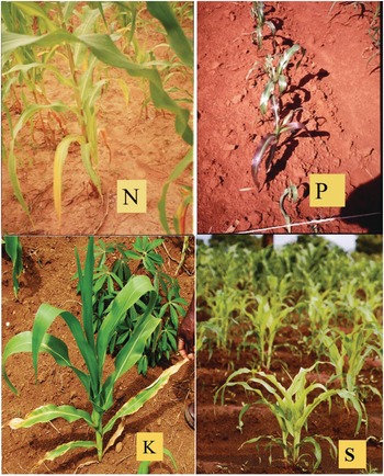
Fig. 12.1 Maize deficiency symptoms of the four main limiting macronutrients in the tropics. Nitrogen (N) deficiency in southern Malawi; phosphorus (P) deficiency in western Kenya; potassium (K) deficiency in Nigeria; and sulfur (S) deficiency in northern Malawi.
Soil fertility is the capacity of soils to supply essential nutrients to plants. Currently, we recognize 17 elements as essential plant nutrients, three of which, carbon (C), oxygen (O) and hydrogen (H), are taken up from the air and soil pores, and the remaining 14 from the soil. Essential means that without them plants, microbes or animals would not be able to complete their life cycles (Barker Reference Barker2010). Essential elements are not fungible; it is not possible to substitute one for another, all are equally essential. Table 12.1 lists them in order of their typical concentration in plants, indicating the main ionic or molecular species that plants take up, and their main functions in plant physiology.
Table 12.1 The essential nutrient elements, in order of typical concentration in plants. Adapted from Barker (Reference Barker2010) and Muñiz (Reference Muñiz2008).
In addition, there are other elements that are considered beneficial but not essential – silicon (Si), iodine (I), selenium (Se), chromium (Cr), vanadium (V), arsenic (As), sodium (Na), and cobalt (Co) being the main ones. Silicon imparts strength to plants to stand up straight and deters some chewing insects, but high contents can damage milling machinery. Some grasses (rice, sugar cane) respond to silicon in Oxisols and Histosols that have very low levels of layer-silicate clays or weatherable minerals. Iodine is an essential element for humans to develop intelligence early in life, and is treated as one of the five “micronutrients” in human nutrition (Chapter 2). Selenium is very important in animals and is commonly a component of salt licks that are used in livestock production. It is also important in wheat growth (Ivan Ortiz-Monasterio, personal communication, 2016). Chromium, vanadium and arsenic are also considered essential elements for animals (Muñiz Reference Muñiz2008). Sodium is everywhere in fluids of living beings, but its essentiality has not been proven. However, sodium is believed to be required for nitrogen fixation.
While this list seems overwhelming, nature takes care of most of these plant requirements with little help from humans, who focus on managing nutrients that are deficient, or in some cases those that can reach toxic levels (iron, manganese, boron, sodium), as well as occasional interactions between calcium, magnesium and potassium. Note that aluminum (Al) is not a nutrient, but often reaches toxic levels in acid soils. Environmentally, carbon (CO2, CH4), nitrogen (NO3–, N2O, NO) and phosphorus (H2PO4–, HPO42–) can harm the environment, causing global warming or eutrophication.
There are three main principles of soil fertility: the law of the minimum, synchrony and nutrient cycling.
12.1 The Law of the Minimum
Justus von Liebig (Reference Sanchez, Palm, Szott, Cuevas, Lal, Coleman, Oades and Uehara1840) established the law of the minimum, which states that plant growth will be limited by the essential element that it is most deficient in. So, if it is nitrogen – as is mostly the case – plants will respond to nitrogen applications until a plateau is reached. Then if phosphorus is the second most limiting nutrient, additional growth will take place with phosphorus fertilization until a yield plateau is reached, and so on. If the limiting factor is physical, such as soil compaction, plants will not respond adequately until that constraint is largely overcome. Even if levels of all 14 nutrients are adequate, growth may be limited by water, the genetic potential of the crop’s cultivar, management and, ultimately, by temperature and solar radiation. The law of the minimum is shown in Fig. 12.2, and is the first principle of soil fertility.
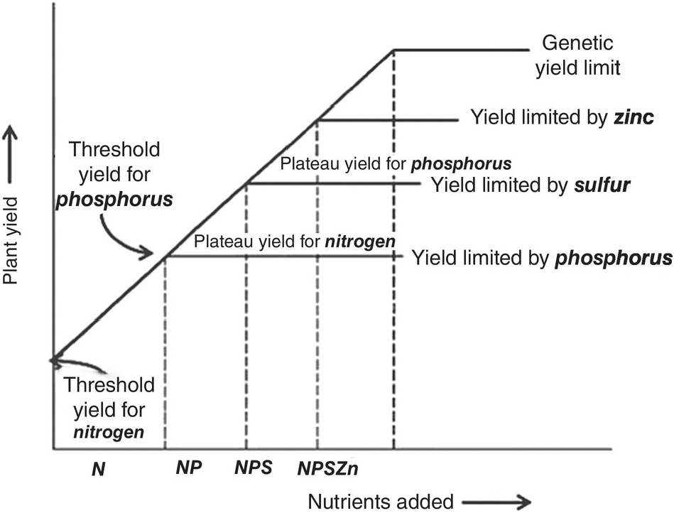
Fig. 12.2 Illustration of the law of the minimum.
12.2 Synchrony
Unlike the law of the minimum, which shows a linear response with plateaus, the time course of plant nutrient uptake (nutrient accumulation) is a parabolic curve. It is very flat at the beginning, mostly because the seedling is using seed reserves, then shows a slow growth while plants build up their root system, then a “grand” period of rapid growth, then a slowing down as plants switch to their reproductive stage, which is followed by a plateau and, in certain cases, a decrease, as physiological maturity approaches (Fig. 12.3).
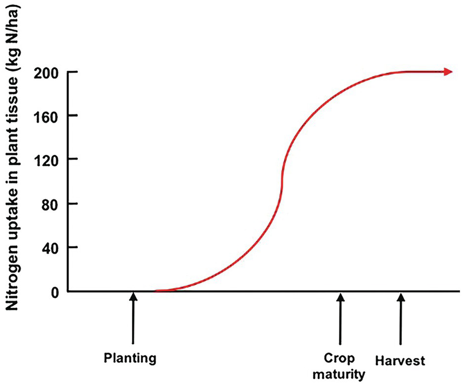
Fig. 12.3 A typical nutrient-uptake curve.
The ideal way is to synchronize nutrient additions with the plant’s nutrient requirements as it grows. This is the “synchrony principle,” developed under the leadership of ecologist Mike Swift (Swift Reference Swift1985), and is the second principle of soil fertility; one which represents the agronomist’s dream, and is seldom, if ever, realized.
The difficulties in synchronization are caused by two main reasons. First, there is the total asynchrony between the germinating seedling and basal fertilizer applications before or at planting. The seedling, as mentioned before, draws nutrients from its seed reserves and is incapable of using any basal fertilizer, which is vulnerable to leaching until the root system develops. In the case of nitrogen, basal applications are also vulnerable to denitrification and nitrous oxide (N2O) emissions to the atmosphere, and to ammonia (NH3) volatilization in soils with high pH. The second reason is the pulse effect of soluble fertilizer applications, as soluble mineral fertilizers, when exposed to soil moisture, drastically increase the ionic content in the soil solution of the nutrient in question. This lack of synchrony is shown in Fig. 12.4. This figure shows the crux of the nutrient efficiency issues, a central challenge of soil management, and one now recognized to be a major player in global warming due to N2O emissions to the atmosphere.
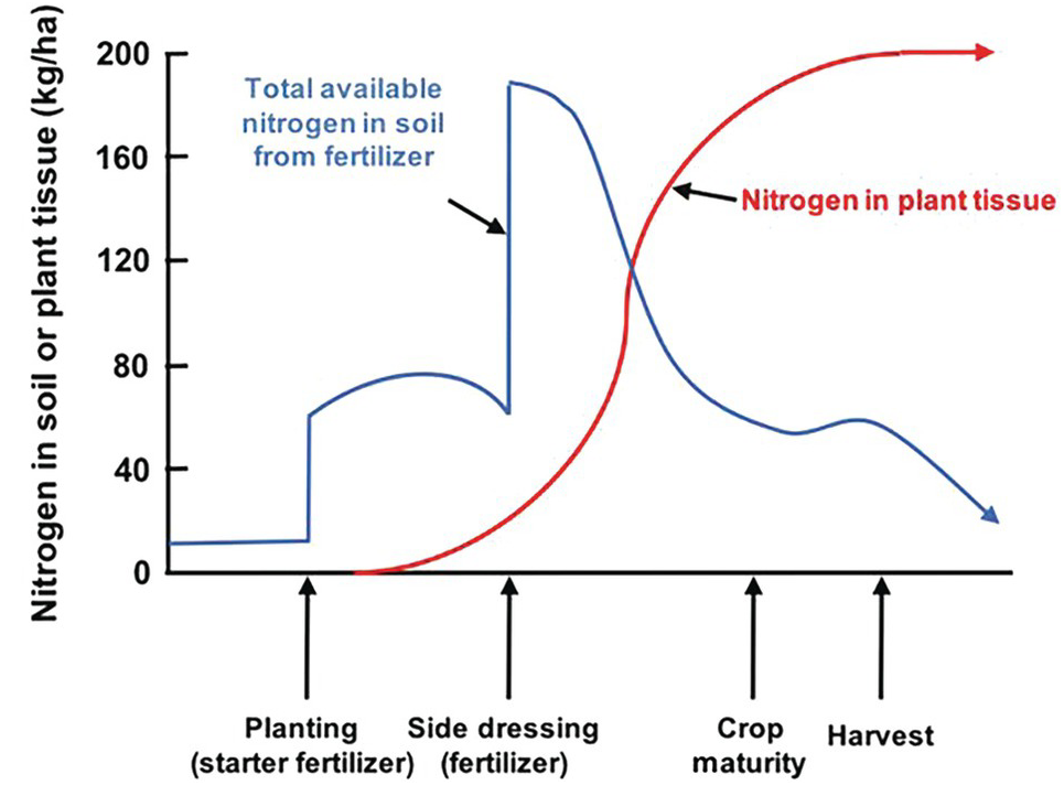
Fig. 12.4 Synchrony between a crop nutrient uptake pattern and fertilizer application is very difficult to achieve, especially at the early stages of growth.
12.3 Nutrient Cycling
Nutrient cycling is the third fundamental principle of soil fertility. Vitousek et al. (Reference Vitousek, Hättenschwiller, Olander and Allison2002) noted the following salient point: cycles of soil nutrient elements are different, varying in speed depending on the types of bonds the elements have with carbon, and on their stoichiometry (element ratios). Organic nitrogen (N) forms covalent bonds with organic carbon (C) (–C–N–), while organic phosphorus (P) and organic sulfur (S) form ester bonds (–C–O–P or –C–O–S), and most other nutrient elements (potassium [K], calcium [Ca], magnesium [Mg], iron [Fe], manganese [Mn], zinc [Zn], etc.) are either bonded ionically or are in loose associations with soil organic carbon (SOC).
The covalent bonding of N with C results in a series of soil organic nitrogen (SON) compounds that are chemically recalcitrant or physically protected in the slow and passive SON pools. Phosphorus and sulfur compounds have a high negative charge, which is believed to prevent them from being entrapped in the slow and passive SOC pools, confining them to the “active” SOC and the structural and metabolic carbon organic input pools. The ester links between organic phosphorus and organic sulfur are readily split by extracellular enzymes, such as phosphatase and sulfatase, which are produced by roots, mycorrhizae and soil microorganisms. Organic phosphorus and sulfur mineralization proceeds rapidly, once the extracellular enzymes break the ester bonds. The resulting phosphorus and sulfur anions react with soil minerals in ways that nitrogen does not.
This makes nitrogen mineralization slower and more costly in terms of energy (supplied by carbon) than the mineralization of phosphorus and sulfur. In terms of stoichiometry, plants have C:N ratios of 100 and above, while soil bacteria have low C:N ratios, about 6, which means that bacteria require more nitrogen relative to the energy available, and in fact they are usually nitrogen-starved. Phosphorus and sulfur cycles are more flexible than the nitrogen cycle (Vitousek et al. Reference Vitousek, Hättenschwiller, Olander and Allison2002).
Also, nutrient cycles vary in how closed or “tight” they are because of different loss pathways. The nitrogen cycle is very “leaky” because of gaseous and leaching losses. The phosphorus cycle is “tight,” but the potassium cycle is also leaky. The question of how to loosen or tighten nutrient cycles in agricultural systems is a priority for soil scientists.
12.4 Nutrient Uptake by Crops and Cycling
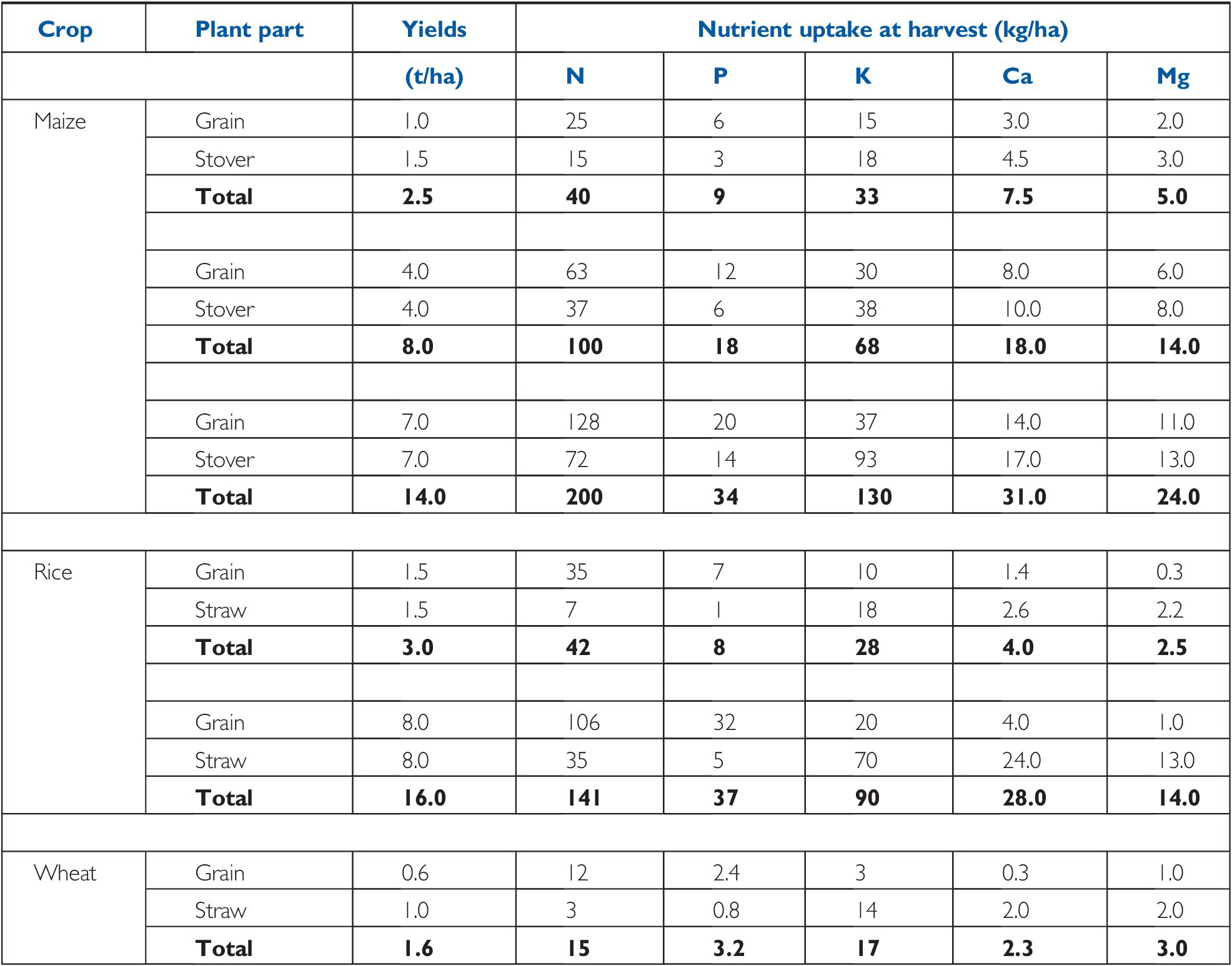
The demand side of soil fertility is best represented by the nutrient uptake at harvest. Tables 12.2 and 12.3 give useful information on crops at different yield levels and their nutrient uptake. For industrial and fruit crops, only the nutrients actually removed from the field are indicated (Table 12.4).
Table 12.2 Nutrients accumulated by major cereals, in yields of cereals on a dry weight basis (12–14 percent water). Typical values.
| Crop | Plant part | Yields | Nutrient uptake at harvest (kg/ha) | ||||
|---|---|---|---|---|---|---|---|
| (t/ha) | N | P | K | Ca | Mg | ||
| Maize | Grain | 1.0 | 25 | 6 | 15 | 3.0 | 2.0 |
| Stover | 1.5 | 15 | 3 | 18 | 4.5 | 3.0 | |
| Total | 2.5 | 40 | 9 | 33 | 7.5 | 5.0 | |
| Grain | 4.0 | 63 | 12 | 30 | 8.0 | 6.0 | |
| Stover | 4.0 | 37 | 6 | 38 | 10.0 | 8.0 | |
| Total | 8.0 | 100 | 18 | 68 | 18.0 | 14.0 | |
| Grain | 7.0 | 128 | 20 | 37 | 14.0 | 11.0 | |
| Stover | 7.0 | 72 | 14 | 93 | 17.0 | 13.0 | |
| Total | 14.0 | 200 | 34 | 130 | 31.0 | 24.0 | |
| Rice | Grain | 1.5 | 35 | 7 | 10 | 1.4 | 0.3 |
| Straw | 1.5 | 7 | 1 | 18 | 2.6 | 2.2 | |
| Total | 3.0 | 42 | 8 | 28 | 4.0 | 2.5 | |
| Grain | 8.0 | 106 | 32 | 20 | 4.0 | 1.0 | |
| Straw | 8.0 | 35 | 5 | 70 | 24.0 | 13.0 | |
| Total | 16.0 | 141 | 37 | 90 | 28.0 | 14.0 | |
| Wheat | Grain | 0.6 | 12 | 2.4 | 3 | 0.3 | 1.0 |
| Straw | 1.0 | 3 | 0.8 | 14 | 2.0 | 2.0 | |
| Total | 1.6 | 15 | 3.2 | 17 | 2.3 | 3.0 | |
Table 12.3 Nutrients accumulated by root and grain legume crops and forage grasses. Root crops are in fresh weight, grain legume in grain yields, as for cereals in Table 12.2, grasses in above-ground dry mass. Typical values.
Table 12.4 Nutrients removed by major industrial and fruit crops. Typical values. From first edition.
In nutrient cycling, there are major differences in how much of the nutrients tropical ecosystems take up and return to the soil. Table 12.5, complied by a team of ecologists and agronomists (Sanchez et al. Reference Sanchez, Gavidia, Ramirez, Vergara and Minguillo1989), illustrates several key points. Tropical rainforests, both on acid and fertile soils, produce more than twice (~4 t C/ha per year) the above-ground litter than tropical savannas. Only high-input wetland rice and a maize–maize–soybean system produced similar annual amounts. But the champion of them all was the white potato in the Andes, which produced almost 7 t C/ha of tops in only 4 months. The lowest value was ~0.4 t C/ha of sorghum stover in the Sahel.
Table 12.5 Biomass and nutrient uptake of above-ground organic resources that are recycled back to the soil in tropical natural systems and agroecosystems, assuming total residue return, but the economic parts were harvested. Representative values. Adapted from Sanchez et al. (Reference Sanchez, Gavidia, Ramirez, Vergara and Minguillo1989).
| System description and duration (in parenthesis) | Economic yield (t/ha) | Yield: residue ratio | Input | Dry biomass (t/ha) | Nutrients returned to soil (kg/ha) | ||||
|---|---|---|---|---|---|---|---|---|---|
| Ca | N | P | K | Ca | |||||
| Natural systems (1 year): | |||||||||
| Tropical rainforest, acid soilsb | – | – | Litter fall | 8.8 | 3960 | 108 | 3 | 22 | 53 |
| Tropical rainforest, fertile soilsc | – | – | Litter fall | 10.5 | 4725 | 162 | 9 | 41 | 171 |
| Tropical savannad | – | – | Litter fall | 3.8 | 1719 | 25 | 5 | 31 | 11 |
| Short-cycle tropical food cropsc: | |||||||||
| Rice (4 months)e | 2.2 | 0.8 | Straw | 2.8 | 1260 | 15 | 2 | 37 | 11 |
| Maize (4 months)f | 1.3 | 0.7 | Stover | 2 | 900 | 18 | 3 | 19 | 7 |
| Sorghum (5 months)f | 0.7 | 0.8 | Stover | 0.9 | 405 | 8 | 1 | 10 | 4 |
| Potato (4 months)f | 10.7 | 0.7 | Tops | 15.1 | 6975 | 17 | 1 | 43 | 14 |
| Soybean (3 months)g | 1.7 | 0.7 | Stover | 2.4 | 1080 | 27 | 2 | 24 | 22 |
| High-input tropical agroecosystems: | |||||||||
| Wetland rice, two crops per year (1 year)e | 11 | 1 | Straw | 11 | 4950 | 59 | 9 | 151 | – |
| Maize–maize–soybean, three crops per year (1 year)h | 8.7 | – | Stover | 9.3 | 4185 | 139 | 15 | 98 | – |
| Soybeans, Cerrado (4 months)g | 2.3 | 0.7 | Stover | 3.5 | 1575 | 86 | 8 | 43 | – |
| Cocoa/Erythrina agroforestry, Brazil (1 year)i | 1 | 0.2 | Leaf litter | 6 | 2700 | 81 | 14 | 71 | – |
| Low-input tropical agroecosystems: | |||||||||
| Upland rice–rice–cowpea, Peru (1 year)i | 4.7 | – | Straw/ stover | 6 | 2700 | 77 | 12 | 188 | – |
| Brachiaria humidicola/Desmodium ovalifolium grazed pasture, Colombia (1 year)j | – | – | Leaf litter | 7 | 3153 | 60 | 5 | 12 | – |
| Alley cropping, Inga edulis (1 year)k | – | – | Tree prunings | 6 | 2700 | 137 | 10 | 52 | – |
| Cocoa/Erythrina agroforestry, Brazil (1 year)i | 1 | 0.2 | Leaf litter | 6 | 2700 | 81 | 14 | 71 | – |
a Vitousek and Sanford (Reference Vitousek and Sanford1986).
b Sarmiento (Reference Sarmiento1984).
c Nutrient contents from DeDatta (Reference DeDatta1981).
d Yields for the tropics from the FAOSTAT statistics database (fao.org/faostat), data for 1985, accessed in 1989.
e Nutrient content from first edition.
f Yields from Goedert (Reference 325Goedert1986), nutrient content from Henderson and Kamprath (Reference Henderson and Kamprath1970).
g First edition; Sanchez et al. Reference Sanchez, Villachica and Bandy1983; TropSoils (Reference Caudle and McCants1987).
h CEPLAC (1989).
i Sanchez and Benites (Reference Sanchez and Benites1987).
j CIAT (1985).
k Szott (Reference Szott1987).
High-input agroecosystems generally add similar nutrient inputs to the soils as the natural systems. For example, residues returned to the soil by an annual maize–maize–soybean rotation in the Peruvian Amazon provided more nitrogen, phosphorus, potassium and similar levels of calcium and magnesium than litter fall from a tropical rainforest in similar soils. Residue return in intensive wetland rice production exceeded nutrient litter fall, particularly for potassium, compared to a tropical rainforest on fertile soils. Fertilizer and liming applications in these high-input systems is a principal reason for this.
As expected, this did not happen in low-input systems, but when aluminum-tolerant cultivars were used in acid soils, some systems came surprisingly close to the natural ones. The upland rice–cowpea rotation, after burning a secondary forest, recycles less carbon and nitrogen, but more phosphorus and much more potassium than the rainforest in similarly acid soils. The aluminum-tolerant Brachiaria humidicola/Desmodium ovalifolium grazed pasture in the Colombian Llanos returned more carbon, nitrogen and calcium, similar levels of phosphorus and magnesium, but less potassium, than the natural tropical savanna systems (Sanchez et al. Reference Sanchez, Gavidia, Ramirez, Vergara and Minguillo1989). This indicates that well-managed, fertilized agricultural systems can recycle nutrients back to the soil similarly to the appropriate natural system, even though the economic product, principally grains, have been taken away. The trick is to ensure that crop residues are returned to the soil.
12.5 Determining Fertilizer Needs
The three soil fertility principles are used as the basis for determining mineral and organic fertilizer needs – one of the major agronomic challenges, not only for increasing food production, but also to reduce leaching and greenhouse gas emissions.
The previous section dealt with the demand side, or the amounts of nutrients needed by plants, as well as the nutrients returned to the soil by cycling. Now we turn to the supply side, determining how much mineral fertilizer is needed (organic fertilizers are discussed in Chapters 11 and 13). The main steps to determine fertilizer needs are soil sampling, tackling variability, laboratory analyses, soil test correlations, modeling and developing fertilizer recommendations.
12.5.1 Soil Sampling
Taking a representative soil sample is both the first step and the largest source of error in soil fertility evaluation, because of the magnitude of extrapolation of the analytical results. When a 5-g subsample taken from a 500-g composite sample of a 2.5-ha field at 15-cm depth is used for phosphorus determination, it represents one-billionth (10–9) of the total soil volume for which the analysis is made (Perur et al. Reference Perur, Subramanian, Muhr and Ray1974).
Soil scientists assume that the distribution of printed instructions and diagrams on how to take soil samples is sufficient to be assured of representative specimens. Unfortunately, this is not always the case. A representative soil sample is a composite of 10–20 samples of the root zone of a field with no major variation in slope, drainage, color or past fertilizer history. For deep-rooted plants, I recommend taking a 0–20-cm and 20–50-cm sample, and for the deepest rooted ones, a 50–100-cm and 100–300-cm sample. Non-representative areas, such as fence rows, termite mounds, those where straw has been burned and manure piles must be avoided. Appropriate information is also needed, including the name and address of the farmer, georeference, previous crop, and fertilizer practices. This is best provided with a web-based questionnaire in the local language that can be sent electronically to a central laboratory. An example for maize-growing in Mindanao, Philippines, has been successfully developed by the International Rice Research Institute (IRRI 2011).
For established pastures or permanent crops where fertilizers are not likely to be incorporated, sampling the top 20 cm is usually sufficient. For nitrate analysis, the 20–50-cm subsoil is usually sampled, and nitrate sampling tools and procedures exist. Subsoil samples, to at least 50 cm and beyond, are important in oxidic subsoils for estimates of anion exchange capacity, gypsum requirements and deep SOC.
Another important question is where to sample when phosphorus has been applied in bands. The answer is between the bands, if their locations are known. The same is true for conservation tillage. A third consideration is the time of the year. Soil samples should be taken a long time before planting so that the results will be available when the decision is made as to how much fertilizer is to be applied. In ustic soil moisture regimes, this means sampling during the dry season, when upward ion movement takes place. This may change some of the soil test results, principally in regard to potassium.
How often a field should be sampled depends on the intensity of fertilizer use and the economic value of the crop. For average management intensity, once every 3 years has been recommended by the International Fertilizer Evaluation and Improvement Program (ISFEIP; 1967–1974), while for very intensively managed areas, annual sampling is necessary. In my opinion, deep soil sampling in oxidic soils should be carried out once every 5 years, or at a changing point in a rotation. Deep sampling and related shallower sampling can estimate changes in soil carbon at that time.
As soil testing is a service program, the time between soil sampling and its analysis should be minimized. As emphasized in the first edition, delays in shipping, power failures and the absence of some reagents in many tropical laboratories are unfortunately very common. Several studies have been made on the effect of time in storage and drying on analytical results. This is still valid, four decades later, in much of the tropics.
After arrival at the laboratory, the soil sample is dried, then ground, either by pounding or by electric-powered grinders, passed through a 2-mm sieve, and assigned a laboratory number or stored until ready for analysis. Bouldin et al. (Reference Bouldin, Greweling and Lui1971) studied the effect of drying versus keeping several Oxisols and Ultisols moist for a period of months. Drying decreased the exchangeable aluminum ion (Al3+) content by 20 percent and increased the exchangeable ammonium (NH4+) content when both were extracted by 1 M KCl. No changes in pH, available phosphorus, calcium or magnesium were observed.
12.5.2 Tackling Soil Variability
Spatial variability in soil properties is always an issue because soil is far from a homogeneous system and bears the footprints of generations of farmers who add temporal variability. The question is how wide-ranging is the variability. I have seen thousands of hectares of very uniform soils that follow a predictable pattern due to landscape position in Oxisols of South America, where large-scale farming is practiced. The uniformity of these soils results from the deep, weathered sediments that they are derived from; variability of these soils is minimal, and is found mainly along slopes. Local extension workers recommend sampling every tens or hundreds of hectares, every few years.
The mixing and leveling of flooded and puddled rice soils for decades or centuries in Asia acts essentially like the blender we use in our kitchens, making a pretty uniform slurry. Variability is thus minimized. At the other extreme, in smallholder farms in Africa, the human footprint is enormous. Lots of natural spatial variability exists in a mosaic of soils due to the topography and because the soils are derived from different kinds of rock, and also from management, as illustrated in Fig. 12.5. When people farm 1 or 2 hectares, they get to know their fields very well, and such knowledge helps in determining where to sample.
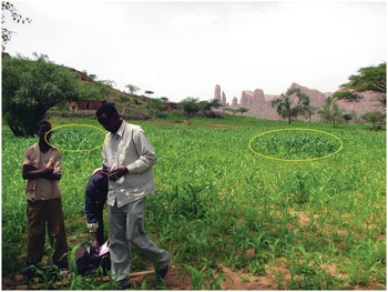
Fig. 12.5 In-field variability in a maize field in Koraro, Ethiopia.
Fields close to the household (infields) are usually more fertile than those farther away (outfields) because smallholder households dump garbage and kitchens ashes, and their domestic animals often urinate and defecate in these nearby fields. This results in a fertility gradient, illustrated in Fig. 12.6, using a portable pH meter.
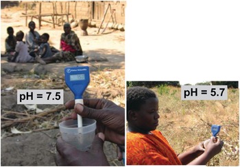
Fig. 12.6 Home garden soils are almost always much more fertile than soils in the larger fields away from home. Mbola, Central Tanzania.
12.5.3 Laboratory Analysis
The most widely used way to assess the status of a nutrient in a soil is by an extraction in a wet chemistry laboratory. Soils are shaken with an extractant, which is supposed to indicate in a few minutes the amount of a nutrient a typical crop would take up from the soil over its lifetime. These values are variously known as available phosphorus, potassium, etc., usually including the name of the procedure’s author (Olsen, for example). Water is also used as an extractant, and resin, to capture ions in a soil slurry. All these extracted products are artifacts (like humic or fulvic acids), which makes them difficult to relate to reflectance spectrometry on the whole soil, but when they correlate with plant growth, they become useful metrics. Because of its mobility in soils, there are no similar soil tests for nitrate nitrogen (nitrate-N).
The wet chemistry laboratory is the backbone of a soil testing program. Unlike research laboratories, service laboratories must be geared to handle large numbers of samples, rapidly and accurately. A complete system of semi-automated apparatus was developed by the ISFEIP for tropical laboratories in the 1970s and 1980s. This system is summarized below, abstracted from the first edition of this book, when ISFEIP was being rapidly scaled up in Latin America and India. Other models are now in place.
Soil samples are measured volumetrically, eliminating the time-consuming weighing process, and then placed in multiple-unit trays, where the extracting and diluting solutions are added or transferred by specially designed diluter-dispensers. Other apparatus transfers the aliquots to spectrophotometers and pH-measuring units automatically. Shaking, stirring and cleaning apparatus are also semiautomatic and capable of handling 30 units at a time. A single technician can run 100 soil samples a day, measuring 10 determinations per sample. The pieces of apparatus are based on manual operation and use a minimum of electrical power. Expensive electronic equipment, such as atomic absorption spectrophotometers, is used only during the last stages. An additional advantage is that the same units can be used for plant tissue as for soil analysis.
The bulk of the work is done with two extractants: the dilute double acid (Mehlich) or the modified Olsen extractant for determining available phosphorus, potassium, calcium, magnesium, sodium, iron, manganese, zinc and copper; and the 1 M KCl extraction for aluminum. Routine tests for nitrogen, boron, sulfur and molybdenum could not be adapted to the system.
12.5.4 Soil Test Correlation
A soil test value per se is worthless; it is an empirical number that may or may not indirectly reflect nutrient availability, and as mentioned before, what is measured is an artifact of the extraction procedure. Soil test values become useful only when they are correlated with crop responses. Such correlations are usually conducted at two levels: an exploratory one in the greenhouse with a large number of widely diverse soils, and a more definite one in the field with fewer, but carefully selected, soils. Correlations can be done in many ways, using fairly complicated formulas, but in my view the simplest and most practical one is to plot relative yields versus the soil test levels as a scatter diagram. Then simply use a transparent overlay with a cross, placing it where the number of points in the upper left quadrant and in the lower right quadrant are at the minimum. This Cate–Nelson method (Cate and Nelson Reference Cate and Nelson1971) gives the soil critical level, as illustrated in Fig. 12.7. (I am sure a software program has been developed to do the same.)

Fig. 12.7 The Cate–Nelson method for determining the critical soil test level. In this case the critical level is 6 ppm available phosphorus by the Bray 1 method, for sugar cane, in the State of Pernambuco, Brazil. Each dot represents a field plot
This concept of a “critical value” for a given soil and farming system has important practical implications for efficient phosphorus use. Maintaining the soil at or close to the critical value has important benefits to the farmer (in terms of economic return) and to the environment, in terms of reducing the risk of phosphorus transfers to surface waters (Syers et al. Reference Syers, Johnston and Curtin2008).
The Cate–Nelson method also tells us the points with a high probability of a phosphorus response (the lower left quadrant), and those with a low probabiliy of phosphorus response (in the upper right quadrant). It does not tell you how much fertilizer to add, but it tells you whether you need it or not. This could be improved with better estimates of uncertainty.
If the soil in question is above the critical level, the decision is clearly not to apply that particular nutrient element to that crop. If the soil is below the critical level, then the decision becomes how much to apply. This requires yield response field trials. There are two main types of models to express yield response curves: the classic curvilinear model and the simpler linear reponse and plateau model.
12.5.5 Curvilinear Models
These classic models are based on the law of diminishing returns, where curvilinear functions (quadratic, square-root, logarithmic, Mitscherlich, etc.) are fitted to the yield response data. Statistical techniques determine which function fits the data best by providing the highest coefficient of determination (R2). The optimum fertilizer rate is determined at that point where marginal revenue equals the marginal cost (i.e. the point where the price of the last yield increment equals the cost of the last increment of fertilizer). The point can be determined mathematically or graphically by drawing a price:cost ratio line, expressed in the agronomic equivalents in the yield response diagram. The optimum yield is then determined at the point where a tangent of the price:cost ratio line intersects the response curve. When more than one element is deficient, regression models take this into account, as well as the interactions between these elements. The recommended rates are determined by solving simultaneous equations.
Curvilinear models are also used in a different manner to produce one function that takes into account soil test levels as variables, as well as other variables related to soil, climate and management properties, in an attempt to account for the uncontrolled variables. A yield equation relating potato yields in Peru needed 27 variables (Ryan and Perrin Reference Ryan and Perrin1973). Optimum fertilizer levels are calculated on the basis of levels of crop prices, fertilizer costs, expected rainfall and soil properties.
Such complex models are effective when there is adequate information about the variables involved and when prices are stable. They fail in the tropics where there are insufficient data to quantify all variables. The use of complex models in tropical regions is limited to after-the-fact analysis in areas with detailed information; they do not serve successfully as predictive tools. In addition, Anderson and Nelson (Reference Anderson and Nelson1975) found that quadratic models are biased when there is a marked response to the first fertilizer increment, followed by little or no response at higher rates. In such cases, optimum fertilizer recommendations became unrealistically high.
12.5.6 The Linear Response and Plateau Model
A series of studies conducted in England by Boyd (Reference Boyd1970) and in the United States by Bartholomew (Reference Bartholomew1972) summarized many fertilizer response functions over the world and concluded separately that in most instances fertilizer response curves can be characterized by a sharp linear increase followed by a flat horizontal line. Bob Cate and Larry Nelson in North Carolina then developed the Linear Response and Plateau model (LRP), which is also based on Liebig’s law of the minimum, and is a logical extension of the Cate–Nelson correlation model (Waugh et al. Reference Waugh, Cate, Nelson, Manzano, Bornemisza and Alvarado1975). Fertilizer response from a field, or a group of fields, is represented in this model by two straight lines for each nutrient. The first line represents the relatively steep response of an added nutrient until it ceases to be a major limiting factor. This is followed by a line showing a flat plateau, where further additions no longer increase yields. The fertilizer response curve so constructed consists of two main points. The “threshold yield” is the yield at the zero level of the nutrient in question, but not of all nutrients. The “plateau yield” is the yield at the point where the nutrient ceases to be a limiting factor; it is not the maximum yield because other factors may still limit yields. The fertilizer rate needed to reach the plateau yield is the recommended rate for the particular nutrient.
The comparison between the two approaches is shown in Fig. 12.8 for the same data set. The dotted lines indicate how the fertilizer recommendations are arrived at. The LRP model has only one optimum point, independent of cost and prices. The curvilinear model shows an optimum point based on the particular price:cost ratio at the time the experiments were conducted.
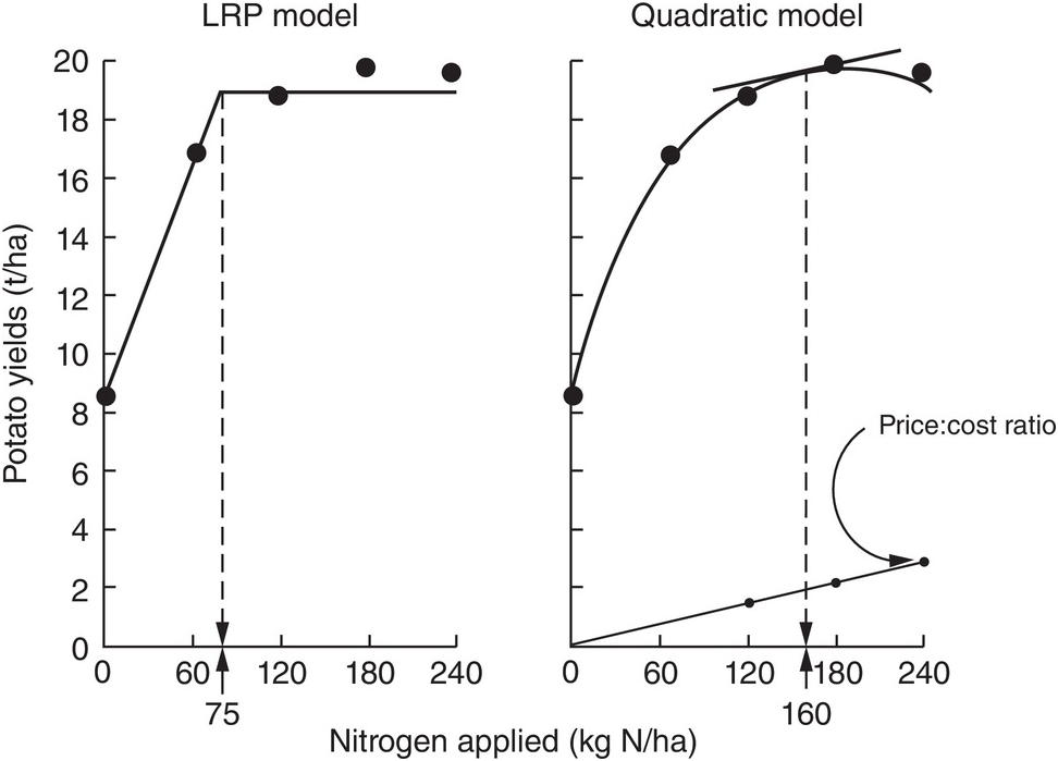
Fig. 12.8 Comparison between the LRP model and the quadratic model using the same field data from potatoes in Peru. The recommended rate is much lower using the first model.
It is very important to note the wide differences in recommended rates between the two methods. The LRP model recommended a lower fertilizer rate (75 kg N/ha) to reach a yield plateau of about 19 t/ha of potatoes. This rate in effect provides nearly maximum yields, while preserving an efficient return per unit of fertilizer, because it is still along the increasing slope. The quadratic model in this case more than doubles the recommendation (160 kg N/ha) in order to obtain only an additional 1 t/ha of yield. This is in the relatively flat part of the curve, where variability is quite high. Small changes in yields result in large changes in recommended rates. In other comparisons, however, the difference in recommended rates might not be as large as in this example.
Which approach is right? I tried it myself with a set of field trials on the response to sulfur-coated urea by wetland rice in the Coast of Peru, where I used the quadratic method (Sanchez et al. Reference Waugh, Cate and Nelson1973). By using the graphic technique, plateau yields and recommended rates were computed. The average nitrogen recommendation in this very high-yielding environment was 224 kg N/ha according to the quadratic model, and 170 kg N/ha with the LRP model. The average gross return for fertilization at the recommended rates was not statistically significant between the two models. The net return per dollar invested in fertilizer was superior with the LRP model.
The LRP model is much simpler, and focuses on the range that provides the most bang for the buck, the linear portion at the threshold yield point. The quadratic models, in their search for the optimum value along the flat part of the response curve, are the least cost-effective. While the science is correct in their case (fertilizer response curves are indeed curves), the practicalities are not, because there is wide variability in the actual results under field conditions. As Bob Cate famously said “If you want to go (from North Carolina) to Tokyo you go via the Great Circle route, but if you want to go from this building to the next, you go in a straight line.” So let’s be as simple and practical as we can.
It is heartening to know that the LRP model is now widely used in US agriculture (Beegle Reference Beegle, Sims and Sharpley2005).
12.6 Early Twenty-First-Century Paradigm Shifts
Building on the advances of the last century, particularly the last quarter of it, three new tools have changed our approach to soil fertility. These are near-infrared spectroscopy, digital soil mapping and bringing the laboratory to the field in scientifically rigorous ways. Together they represent a paradigm shift, not of the science itself, but in how soil science is applied. I am happy to note that the contribution of tropical soil scientists is major in all of the three cases.
12.6.1 Spectrometry
The analysis of wavelengths of light is one of the simplest in physics, and not until the start of this century has it been applied to soil science at scale. Spectrometry has for decades been used as a standard in various industries, such as pharmaceuticals and paints. The near- and mid-infrared wavelengths can be correlated with many, but not all soil properties. In the tropics, the seminal papers by Keith Shepherd and Markus Walsh (Shepherd and Walsh Reference Shepherd and Walsh2002, Reference Shepherd and Walsh2007) showed the value of then near-infrared rudimentary spectrometers that can estimate many soil properties, just by passing light though a soil sample and making the necessary correlations (Fig. 12.9). The main properties that can be determined at present are: sand, silt, clay, organic carbon, exchangeable bases, cation exchange capacity, phosphorus retention and some soil minerals. Where spectrometry does not (yet) work is available phosphorus, potassium and sulfur, very critical soil fertility parameters. Spectrometry is also helpful in determining organic input quality and carbon mineralization rate (Shepherd et al. Reference Shepherd, Vanlauwe, Gachengo and Palm2005).
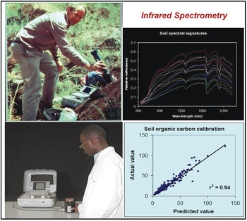
Fig. 12.9 Keith Shepherd (top left) using a portable spectrometer in the field in Kenya, and a technician using it in his Nairobi laboratory (bottom left). The resulting soil spectral signature (top right), and the close correlation between the predicted value by spectroscopy and the “actual” value of SOC from a wet chemistry laboratory (bottom right).
12.6.2 Digital Soil Mapping
Traditional soil maps are composed of polygons (mapping units) and their legends, showing mostly soil classification terms that are of very limited information value to anyone other than a pedologist. Such maps are static and tell you nothing about soil properties. Polygon maps assume that soils are uniform within the mapping unit, which is seldom the case. Interpretations made from them in terms of soil properties and agronomy are of course no better than the map.
To address some of these limitations, a digital soil-mapping working group of the International Union of Soil Sciences (IUSS) started work in 2006, and has since produced valuable information that can be found in books arising from their conferences (Lagacherie et al. Reference Lagacherie, McBratney and Voltz2007, Hartemink et al. Reference Hartemink, McBratney and Mendonça-Santos2008, Boettinger et al. Reference Boettinger, Howell, Moore, Hartemink and Kienast-Brown2010). In 2008, a group of soil scientists, agronomists and ecologists decided to produce a digital map of soil properties and soil functions of the world (Sanchez et al. Reference Sanchez, Ahamed, Carré, Hartemink, Hempel, Huising, Lagacherie, McBratney, McKenzie, Ml, Minasny, Montanarella, Okoth, Palm, Sachs, Shepherd, Vågen, Vanlauwe, Walsh, Winowiecki and Zhang2009, Fisher Reference Fisher2012), and the African portion of that is in progress.
Soil properties are estimated quantitatively with a statistical inference system using spatial (kriging, co-kriging) or non-spatial (regressions, neural networks) techniques, or both, and expressed as their probability of occurrence with uncertainty estimates. They are derived using quantitative relationships between the punctual soil measurements and the spatially continuous soil covariates. This results in maps of soil properties such as the ones selected by the Global Soil Map Consortium as their minimum data set, i.e. clay, organic carbon, bulk density, pH, effective cation exchange capacity, electrical conductivity and bulk density – bulk density is needed to express carbon and nutrients on a mass basis (t/ha) for biogeochemical modeling (Sanchez et al. Reference Sanchez, Ahamed, Carré, Hartemink, Hempel, Huising, Lagacherie, McBratney, McKenzie, Ml, Minasny, Montanarella, Okoth, Palm, Sachs, Shepherd, Vågen, Vanlauwe, Walsh, Winowiecki and Zhang2009). These are the first two actions in the process for developing the digital soil map, as shown in Fig. 12.10. Such properties are mapped on a pixel basis with a resolution as small as 30 × 30 m, which is great for smallholder farms.
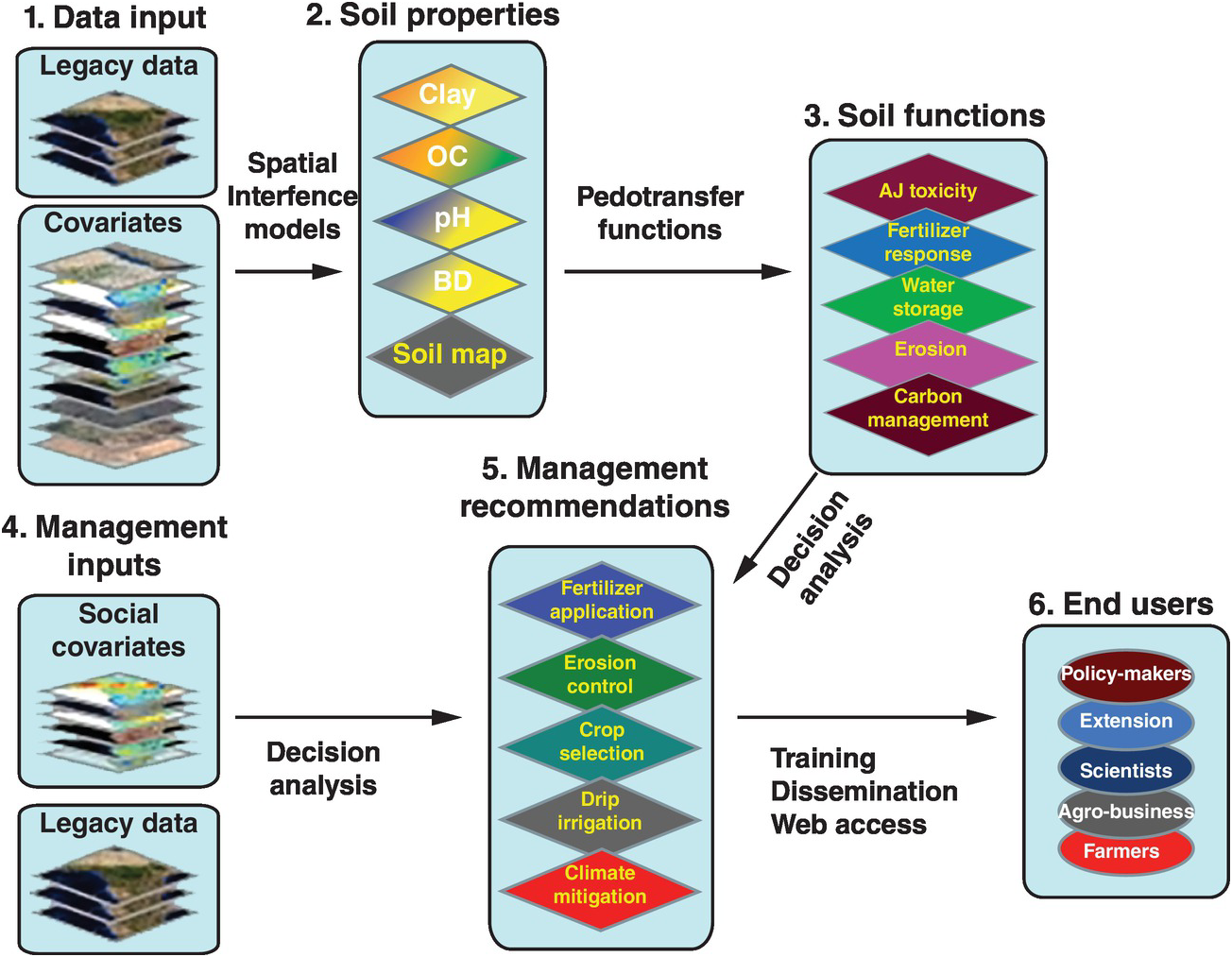
Fig. 12.10 Conceptual flow of the soil digital map process.
The spatially inferred soil properties are then used to predict more difficult-to-measure soil functions (action 3, Fig. 12.10), such as available soil water storage, carbon density and phosphorus fixation, using pedotransfer functions. Rather than calibrating only individual soil properties to infrared spectra, multivariate associations are used to identify soil functions. The overall uncertainty of the prediction is assessed by combining the uncertainties of the input data with the uncertainties of the spatial inference and those of the soil functions, using global sensitivity analysis.
The key is to connect all these soil functions with fertilizer response or other georeferenced field data from well-conducted agronomic experiments (legacy data) as well as with digital maps of population density, roads, distance to markets, internet access and other socioeconomic digital maps (action 4, Fig. 12.10). Analyses of decisions need to be made, connecting the maps with actual on-the-ground experience. Then the final two actions (management recommendations and reaching the end user) can be achieved. Web-based digital soil maps can be made interactive. This is very much work in progress.
12.6.3 Bringing the Laboratory to the Field
Although soil nutrient replenishment in sub-Saharan Africa is widely recognized as a critical biophysical entry point to an agricultural transformation, the actual application of soil science is still minimal, and frustratingly so, in large part because of the delay in obtaining the necessary information from soils sampled in farmers’ fields and sent to a wet-chemistry, conventional laboratory. The data often take a year to come back (if at all) and the paper-based process is prone to errors of recording and transcribing, as well as delays in transmission, interpretation and visualization. Worse still, the data are usually hard to interpret, largely irrelevant and often of questionable quality. The poor infrastructure of Africa and the budget limitations of national institutions are the main reasons used to rationalize this useless exercise. This is not a problem in the more advanced tropical countries, but it is also a problem in many areas outside Africa as well.
The way to get around this is to get the data in situ and send it electronically to the central laboratory where senior people or algorithms make the recommendations and send it back electronically to the extension agent or farmer. The problem is that, up until recently, field soil test kits have proven to be highly inaccurate and not sufficiently precise (Vanlauwe Reference Vanlauwe2008). Weil (Reference Weil2011) of the University of Maryland and Columbia University has been developing a wet-chemistry “SoilDoc,” which has been proven to work well and is highly correlated with central wet-chemistry laboratories (Fig. 12.11). It enables extension workers to make on-the-spot diagnoses of soil constraints, allowing targeted recommendations to advise farmers in real time (Sanchez et al. Reference Sanchez, Weil and Rose2013).
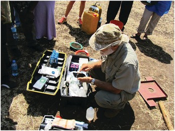
Fig. 12.11 SoilDoc, a “lab-in-the-box” field test kit. Ray Weil is entering the data in a smart phone that transmits it to the cloud or to a central location. Arusha, Tanzania, September 2012.
This tool uses state-of-the-art battery-powered miniaturized instruments, originally created for other purposes such as the beer and swimming-pool testing industries. The soil fertility parameters analyzed include soil pH, electrical conductivity (indicative of general fertility levels as well as salinity issues), biologically active organic carbon, and 0.01 M calcium chloride (CaCl2)-extractable nitrate-N, sulfate-S, phosphate-P, and potassium using specific sensors. Additionally, the kit includes tools to measure soil physical properties such as surface sealing strength, plow pans and volumetric soil water content. Soil texture is estimated by feel. SoilDoc essentially measures what a conventional wet-chemistry laboratory does at a similar level of accuracy (Fig. 12.12) plus biologically active SOC and several physical properties (Weil Reference Weil2011, Sanchez et al. Reference Sanchez, Weil and Rose2013). Like digital soil mapping, this too is very much work in progress.
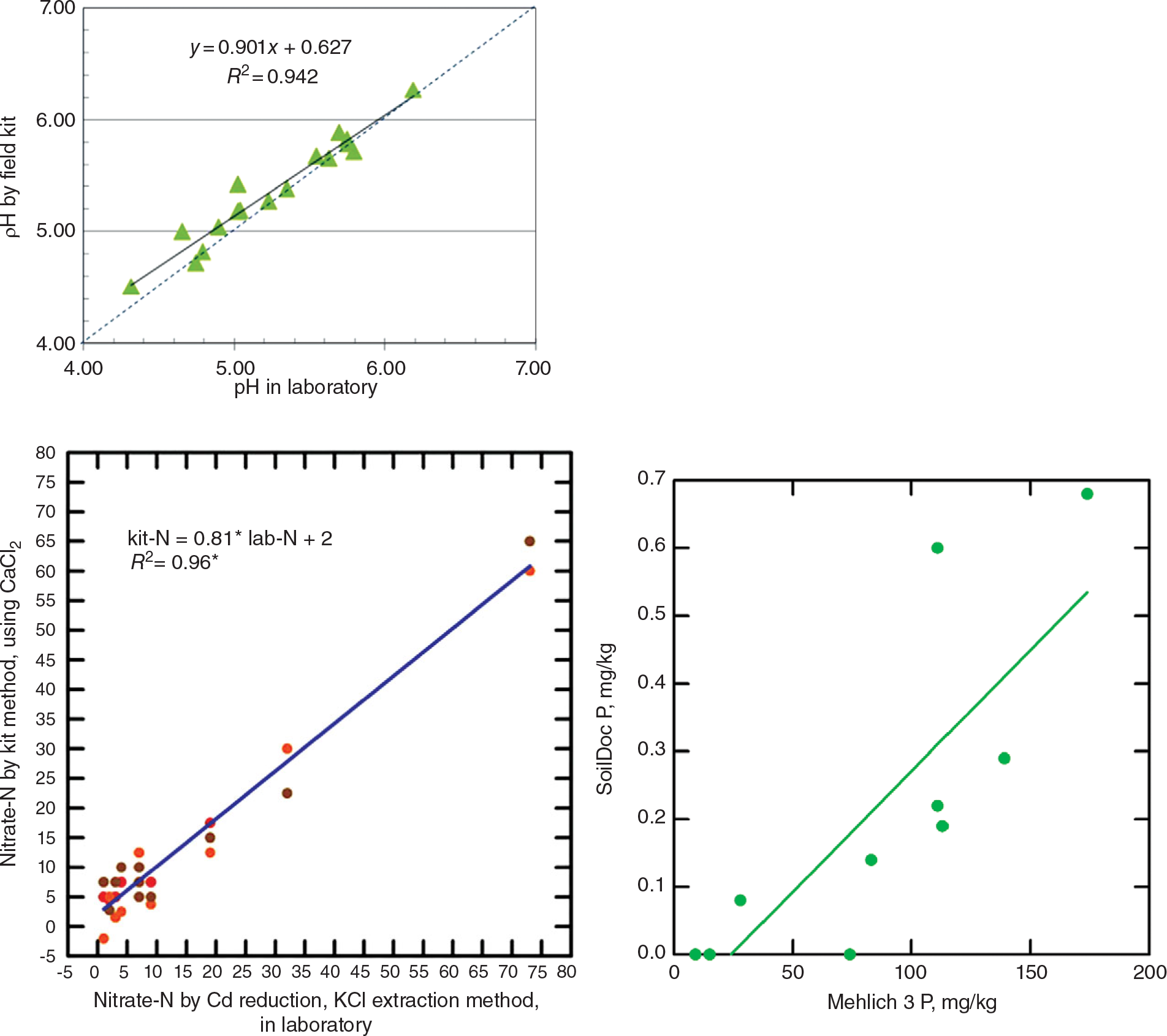
Fig. 12.12 Correlations for pH (top), nitrate-N (middle), and available phosphorus (bottom), determinations by the SoilDoc kit and a wet-chemistry laboratory.
At the time of this writing, we need to use the field-based wet chemistry of SoilDoc and similar systems in conjunction with near-infrared spectrometers, because spectrometry cannot determine available soil test levels since they are artifacts of the extractants used. Wavelength data cannot detect something that does not exist in the soil. To repeat, both approaches are works in progress and their combined use could result in positive synergies.
The combination of these approaches, as well as the rapidly developing soil scanning by satellites, shows tremendous potential for faster and more effective ways of evaluating soil fertility.
12.7 Summary and Conclusions
Soil fertility is the capacity of soils to supply essential elements to plants. Currently we recognize 17 elements as essential plant nutrients. Essential means that without them plants, microbes or animals would not be able to complete their life cycles.
There are three main principles of soil fertility: the law of the minimum, synchrony and nutrient cycling.
The law of the minimum states that plant growth will be limited by the essential element that it is most deficient in.
The ideal is to synchronize nutrient additions with the plant’s nutrient requirements as it grows. This is the “synchrony principle,” which represents the agronomist’s dream, and is seldom, if ever, realized.
Nutrient cycling is the third fundamental principle of soil fertility. Cycles of soil nutrient elements are different, varying in speed, depending on the types of bonds the elements have with carbon.
Organic nitrogen forms covalent bonds with organic carbon, while organic phosphorus and sulfur form ester bonds. Most other nutrient elements are either bonded ionically or are in loose associations with soil organic carbon (SOC).
The covalent bonding of nitrogen with carbon results in a series of compounds that are chemically recalcitrant or physically protected in the slow and passive SOC pools.
Phosphorus and sulfur compounds have a high negative charge which may prevent them from being entrapped in the slow and passive SOC pools. Organic phosphorus and sulfur mineralization proceeds rapidly once the extracellular enzymes break the ester bonds.
This makes nitrogen mineralization slower and more costly in terms of energy (fuelled by soil carbon) than the mineralization of phosphorus and sulfur. In terms of stoichiometry, plants have C:N ratios of 20 and above, while soil bacteria have low C:N ratios, about 6, which means that they require more nitrogen relative to the energy available, and in fact they are usually nitrogen-starved.
It is a priority for soil scientists to accelerate and tighten nutrient cycles in agricultural systems.
The demand side of soil fertility is best expressed as the nutrient uptake at harvest. Different crops exhibit varying yield levels and nutrient uptake.
The high-input agroecosystems generally add similar nutrient inputs to the soils as the natural systems. For example, residues returned to the soil by an annual maize–maize–soybean rotation in the Peruvian Amazon provided more nitrogen, phosphorus and potassium and similar levels of calcium and magnesium than litter fall from a tropical rainforest in similarly acid soils.
As expected, this did not happen in low-input systems, but when aluminum-tolerant cultivars were used in acid soils, some systems came surprisingly close to the natural ones. The trick is to ensure that crop residues are returned to the soil.
Taking a representative soil sample is both the first step and the largest source of error in soil fertility evaluation because it normally represents one-billionth (10–9) of the total soil volume for which an analysis is made.
Spatial variability in soil properties is always an issue because soil is far from a homogeneous system and bears the footprints of generations of farmers who add to it temporal variability.
Fields close to the household (infields) are usually more fertile than those farther away (outfields) because smallholder households dump a lot of garbage and kitchens ashes, and their domestic animals often urinate and defecate in these nearby fields.
The most widely used way to assess the status of a nutrient in a soil is by an extraction in a wet-chemistry laboratory. In modern laboratories, a single technician can run 100 soil samples a day, measuring 10 determinations per sample. The bulk of the work is done with two extractants: the dilute double acid (Mehlich 1) or the modified Olsen extractant for determining available phosphorus, potassium, calcium, magnesium, sodium, iron, manganese, zinc and copper; and the 1 M KCl extraction for aluminum.
Soil test values become useful only when they are correlated with crop yield responses. Correlations can be done in many ways, using fairly complicated formulas. In my view, the simplest and most practical one is the Cate–Nelson method, which plots relative yields versus the soil test levels as a scatter diagram. This method also determines which soils have a high probability of a nutrient response as opposed to those that do not.
There are two main methods to determine the recommended fertilizer rates based on yield response field trials. The first is the traditional curvilinear method, where a quadratic or other function is fit and the point where marginal revenue equals marginal cost represents the recommended rate. The other is the Linear Response and Plateau (LRP) model where yields are represented by two straight lines for each nutrient in the model. The first line represents the relatively steep response of an added nutrient until it ceases to be a major limiting factor. This is followed by a line showing a flat plateau, where further additions no longer increase yields.
The LRP model recommends a lower fertilizer rate, providing nearly maximum yields, while preserving an efficient return per unit of fertilizer, because it is still along the increasing slope. The LRP model is much simpler, and focuses on the range that provides the most bang for the buck. It saves on fertilizer at little yield cost and thus reduces the emission of nitrogen gases and leaching losses, providing a superior net return per dollar invested in fertilizer.
The application of near- and mid-infrared spectrometry can provide accurate estimates of sand, silt, clay, organic carbon, exchangeable bases, cation exchange capacity, phosphorus sorption and some soil minerals. Where spectrometry does not (yet) work is in estimating available phosphorus, potassium, sulfur or nitrogen.
Digital soil mapping is superior to the traditional polygon maps. Digital soil maps, with a resolution of 100-m pixels, can describe soil properties obtained by spectrometry or wet chemistry. The spatially inferred soil properties are then used to predict more difficult-to-measure soil functions, such as available soil water storage, carbon density and phosphorus fixation, using pedotransfer functions. Web-based digital soil maps can be made interactive.
A new generation of field test kits, such as “SoilDoc,” can measure many soil properties using miniaturized wet-chemistry sensors at a similar level of accuracy as large laboratories, eliminating the need to send soil samples to the laboratory, a major obstacle in Africa and other less-developed countries in the tropics. The SoilDoc kit is connected electronically to a central laboratory, sending data in a web-based form, and the recommendations, via algorithms or expert opinion, are returned to the extension agents in real time.