

We are accustomed to thinking of residential property as an asset or an arrangement of legal rights. Yet, property forms are also behavioral, with the property interests and incentives of housing forms enabling or supporting behaviors and commitments. By choosing a residential property form, such as owning or renting, we commit ourselves to a range of opportunities, behaviors, and built-in, ongoing incentives for those behaviors. Homeownership is attractive in significant part for its behavioral and consumption benefits – contrary to the expectations of most homeowners, inflation-adjusted asset appreciation is startlingly modest (Shiller Reference Shiller2015, 27–30). The benefits of homeownership include greater control and governance rights, opportunities for “forced” or automatic savings through mortgages, incentives to maintain and improve property, and stronger rights to stay put.
Viewing property as behavioral, while overbroad, suggests a different starting place for understanding and innovating property forms: focusing on the behaviors we wish to enable and how to produce them. One application is to the rather cramped residential leasehold form, with its shallow possessory rights, weak incentives for property improvement, and limited opportunities for asset building. Can we provide an interested subset of renters a measure of the rights, behaviors, or benefits of homeownership? One way to accomplish this, albeit sometimes coarsely, is to adjust homeownership. A number of proposals in the scholarly literature have sought to create variants of the homeownership form, with the intent of producing some of the behaviors and benefits of homeownership while increasing affordability or adjusting risk (Fennell Reference Fennell2008, 1070–77; Arruñada and Lehavi Reference Arruñada and Lehavi2011, 26–33). There has been less progress in creating alternative housing forms that don’t require equity investment, putting them in reach of lower-income renters.
A behavioral perspective suggests one possibility for innovating rental: the use of incentives and commitment strategies to support alternative property forms and certain ownership-like behaviors and effects. Yet, applying these psychological tools to rental seems an uneasy fit with residential property law, which has tended to rely on equity interests and legal rules to produce ownership effects (e.g., Fischel Reference Fischel2001). Is incentivizing such behaviors inevitably too costly, complex, and vulnerable to unintended motivational effects to be successful?
This chapter examines renter equity, an emerging and understudied intermediate form of housing between homeownership and traditional rental (Cornerstone Renter Equity 2016; Renting Partnerships 2016). This fledging property form, in operation at four affordable housing sites in Cincinnati, Ohio, puts into practice the kind of psychology-informed policy design and finer-grained division of property rights that have been of so much recent theoretical interest (e.g., Fennell Reference Fennell2008, 179–85; Thaler and Sunstein Reference Thaler and Sunstein2008, 3–44). The renter equity form monetizes and allocates to tenants a share of the financial value created by their upkeep and participation in the property – and frames that allocation as an incentive in order to support a range of homeownership-like behaviors and benefits. Specifically, the lease provides renters the right to earn savings credits for a constellation of property-enhancing behaviors (Drever et al. Reference Drever, Brumfield, Decker, Sims, Passty and Wilson2013, 16–20; Renting Partnerships 2016). In turn, the reduced property management and vacancy costs fund the renter savings accounts.
Renter equity has sparked increasing interest and attention from investors, think tanks, and government (HUD 2011; Williams Reference Williams2012, 1–2). Andrea Levere, president of the Corporation for Economic Enterprise, has proposed using HUD funding, including Sustainable Communities Initiative funding, the Community Development Block Grant, and HOME investment partnership funds, to expand the renter equity model on a national scale (Williams Reference Williams2012, 2). The Cornerstone Corporation, which manages three renter equity sites, recently trademarked the name “renter equity,” presumably with an eye toward licensing or franchising it to other providers of low-income affordable housing services. Renting Partnerships, a newer and similar housing form, envisions expanding to a network of affiliates (Margery Spinney, pers. comm.).
In academic circles, renter equity has been a much quieter innovation, with no scholarship to my knowledge addressing this housing form. In this chapter, I examine renter equity as an emerging innovation and a model of the potential, and the pitfalls, of leveraging incentives and commitments to support alternative housing forms. The chapter proceeds in five parts. Part 1 highlights some of the key behavioral options and benefits that renters lack and suggests that one consequence of landlord-tenant reform has been to reduce the incentives and commitment strategies available to tenants. Part 2 describes renter equity and a newer, similar form called renting partnerships. I use the term renter equity throughout this chapter to refer to the core property configuration shared by both renter equity and renting partnerships. Part 3 identifies the conceptual underpinnings of renter equity as well as legal and policy gaps in its implementation. In Part 4, I address behavioral and social concerns about renter equity incentives. Part 5 concludes by briefly discussing renter equity’s potential as an alternative property form and the lessons of renter equity for incentive-based “behavioral leasing.”
8.1 Confines of the Rental Form
Splitting possession from residual ownership (i.e., renting) confers a number of valuable benefits on renters, including greater residential mobility, allocating property management and repair obligations to landlords, and avoiding the financial risks of equity ownership. In other ways, however, this division is binary and often crude from the standpoints of tenant preferences, landlords’ interests, and social and community needs (Fennell Reference Fennell2008, 188–90). Renters, particularly long-term renters, miss out on a number of behavioral options and corresponding benefits allocated to their homeowning counterparts. This section highlights some of the behavioral confines of the rental form.
First, the division of property rights in rental reduces incentives for tenants to maintain and improve the rental property and local neighborhood. Beyond the benefits to consumption, the rental form does not monetize or compensate tenants for their investments in upkeep, safety, or improvements that increase residential value or enhance their local communities (cf. Lerman and McKernan Reference Lerman and McKernan2007, 1–2). Indeed, there are explicit disincentives for such tenant efforts: the risk of increased rent and gentrification (2). In some cases, landlords may compensate tenants implicitly for upkeep and improvements through lower rent. However, the standard lease offers no formal mechanism of compensation on which renters can rely. Concededly, renters have lower consumption motivations for such behaviors because they can exit more cheaply to satisfy consumption elsewhere and have limited control over rental duration (Rohe and Stewart Reference Rohe and Stewart1996, 45). However, renters still engage in some property-benefiting behaviors and presumably would engage in more if they could capture the value of their actions.
Not only do renters lack incentives to invest in property, they typically lack legal rights to do so. Standard residential leases make tenants liable for damages and subject to eviction for altering their units (e.g., appliances, flooring, even wall color) or making repairs without landlord consent. Renters also lack rights to participate in governance and decision making affecting common areas and residential management (cf. Davis Reference Davis2009, 29–31). For some, offloading upkeep and improvement to landlords is an attraction of renting (Freddie Mac 2016, 6, 16). Others, however, desire more intensive participation – perhaps particularly renters who anticipate less attentive landlords or who lack future prospects for ownership. Paucity of control can frustrate tenant preferences, and, some research suggests, produce negative psychological states (Manturuk Reference Manturuk2012, 409–22) and impair control over “image presentation” (Downs Reference Downs1981, 466). It is not surprising, or objectionable, that landlords have strong interests in protecting their property from value dissipation. Yet, some reallocations of consumption-oriented rights to tenants may be possible (e.g., limited tenant decision making subject to standards and a budget or tenant voting within owner-approved choice sets).
Landlord tenant reforms, while salutary in some regards, have narrowed opportunities for tenants to invest and participate in property by creating a harder-edged boundary between possessory rights in rental and ownership interests. In the 1970s, post-industrialization changes in housing needs and failures of rental market competition prompted the “reform era” of landlord-tenant law (Kelley Reference Kelley1995, 1563–74). These reforms shifted the treatment of leaseholds from a conveyance of property to a hybrid of contract and property (Glendon Reference Glendon1982, 503–05; Merrill and Smith Reference Merrill and Smith2001, 820–31). The shift toward contract law enabled courts to impose common law contract doctrines such as unconscionability and the implied warranty of habitability (obligation of the landlord to ensure fit and habitable rental premises), with some of these protections later codified (Korngold Reference Korngold1998, 707–07; cf. Super Reference Super2011, 389–400). These reforms also made many tenant protections non-waivable (Geurts Reference Geurts2004, 356–60).
One consequence of landlord-tenant reform has been to limit tenants’ ability to rent premises more cheaply, improve or maintain them, and realize the value of below-market rent for their lease term. Landlord-tenant laws regulating and limiting escrows (e.g., security deposits) also constrain the ability of tenants to contract with landlords for tenant alterations by escrowing additional money as security against damage. In the face of a complex framework of tenant protections, landlords are leery of contracting for tenants to provide maintenance or repair, make alterations, or assume greater governance or management roles. Even if landlords are willing to engage in such contracting, certain protections, such as the landlord warranty of habitability, cannot be waived in many states (Rabin Reference Rabin2011, 80). In some cases, tenant “sweat equity” arrangements may occur informally. For example, sociologist Matthew Desmond’s ethnography of urban renters describes instances where landlords allowed tenants to make up back rent and avoid eviction by working on the property (Desmond Reference Desmond2016, 129). Landlords who countenance such arrangements risk running afoul of landlord-tenant and labor laws.
A second constraint of the rental form is that renters lack ongoing, long-term rights to stay put. The legal duration of a typical residential lease is one year or month-to-month; after the lease term expires, the landlord can opt not to renew or to increase rent. Unlike homeowners who lock in ongoing possessory rights and a purchase price (and often a mortgage interest rate), tenants face rent increases and the accompanying risk of dislocation (Sinai and Souleles Reference Sinai and Souleles2005, 785–86). The lack of control over housing costs and mobility is a significant drawback to renting that can frustrate tenant preferences, increase psychological stress, and undermine financial security (Desmond Reference Desmond2016). Limited control over residential duration also weakens incentives for tenants to invest in local communities.
Third, tenants have less ability than homeowners to use housing as a commitment device to bind their future selves to certain actions or decisions. Commitment strategies address bounds on willpower and self-control by removing a future temptation or option entirely or raising the costs of exercising that option. The illiquidity of the owned home (i.e., the expense and difficulty of asset transfer) acts as a commitment strategy for longer residential duration and the social, personal, and financial effects that entails. Homeownership also enables buyers to commit at the time of purchase to a hedging strategy against housing cost inflation. Compared to renters, owners pay higher upfront costs to purchase, but face lower risk of housing cost escalation over time (Sinai and Souleles Reference Sinai and Souleles2005, 785–86).
One of the most important “commitment benefits” of homeownership is lodged not in the property form, but in its financing: forced saving. Much of the financial value of homeownership derives not from appreciation, but from long-term homeowners who pay down the principal each month on traditional, self-amortizing mortgages (the most common mortgage choice) (Shiller Reference Shiller2015, 27-30; U.S. Census Bureau 2013, table 1016). The mortgage is a powerful commitment device that makes the consequences of not paying one’s mortgage costly, disruptive, and humiliating. Homeowners accumulate far greater lifetime savings than similarly-situated renters, as a result of the forced saving component of traditional mortgages, homeownership’s relative illiquidity, and its tax subsidy.
Self-amortizing mortgages, which fuse the monthly principal and interest payment into one amount due, create automatic asset-building – an important point in light of the behavioral law and economics research showing marked improvements in saving when contributions are made automatic and set as the default (Benartzi and Thaler Reference Benartzi and Thaler2004, S166-85; Thaler and Sunstein Reference Thaler and Sunstein2008 103–17; cf. Moulton et al. Reference Moulton, Samek, Loibl and Collins2015, 55–74). Of course, lenders can deter or unravel home-based savings with products such as interest-only and negatively amortizing loans, cash-out refinancing, and home equity lines of credit. Saving through homeownership is suboptimal due to these escape hatches and the undiversified nature of the home investment. However, this form of savings has nonetheless proven financially meaningful, as well as culturally resonant and highly attractive to Americans – in large part due to its advantages as a psychological commitment strategy. The dearth of comparable supports for renter asset-building recently prompted Josh Barros to propose that renters self-fund a savings portion, automatically paid on top of their rent, which would be directed monthly to federal MyRA accounts (Barro Reference Barro2014).1
For their part, landlords contend with renters who are, as Julie Roin and Lee Fennell term it, “understaked” to their residential property and the community (Fennell and Roin Reference Fennell and Roin2010, 16–18). The lack of an equity interest and, in some cases, a strong social stake increases delinquent rent, property damage, and turnover. To date, many of the legal tools available to landlords to address these harms are unpopular with tenants (e.g., fees for late rent), expensive and adversarial (e.g., legal process for eviction), or limited to ex-post compensation rather than prevention (e.g., deducting repair costs from the security deposit). In addition, some state statutes limit the penalties that landlords can impose for delinquent rent and other violations (e.g., Cal. Civ. Code § 1671 (d)).
The shortcomings of the rental form have not only frustrated the preferences of a large subset of renters, but have motivated premature and unstable moves to homeownership (Reid Reference Reid2013, 152–54). Some tenants prefer to rent, particularly at earlier and later life stages; however, most report a preference to own (MacArthur Foundation 2014; Pew Research Center 2011). While abundant survey research establishes the strong inclination toward ownership (MacArthur Foundation 2014, 30; Pew Research Center 2011), it is harder to tease from this data relative preferences for different aspects of homeownership.2 The preference to own is likely due in part to government subsidy of ownership, a benefit I do not focus on in this chapter (e.g., Poterba and Sinai Reference Poterba and Sinai2008, 84–89). The desire to stay in place for a longer period of time appears to be an important trigger for homebuying (Sinai and Souleles Reference Sinai and Souleles2005, 785). There is also evidence that renters’ thin control over rental property and inability to build assets through housing drive preferences for homeownership (Rohe and Lindblad Reference Rohe and Lindblad2013, 7–18).
8.2 Producing Ownership Effects through Incentive-Based Leases
Can any of the benefits and behaviors of homeownership be produced for renters, particularly low-income renters without prospects for ownership? A variety of proposals have sought to create more particularized divisions of residential property rights that redistribute the archetypic benefits of renting and homeowning. Lee Anne Fennell has conceptualized this process as “unbundling” property forms to enable valuable divisions of risk and consumption values and proposed a “homeownership 2.0” form to accomplish this (Fennell Reference Fennell2008, 1070–77). Other approaches, such as limited equity cooperatives, focus on increasing homeownership affordability by limiting equity stake to small shares and restricting rights to appreciation on resale (Davis Reference Davis2009, 29–30; Diamond Reference Diamond2009, 88–109). There have also been a number of proposals to redistribute property risks through alternative financing of homeownership. Most prominently, Andrew Caplin has proposed a residential shared appreciation mortgage where a lender contributes a percentage of the total equity needed by the homebuyer in exchange for rights to a percentage of appreciation upon resale (Caplin et al. Reference Caplin, Cunningham, Engler and Pollock2008, 5–11; see also Arruñada and Lehavi Reference Arruñada and Lehavi2011, 26–33).
There has been decidedly less excitement about alternative property forms based in rental. Municipal rent control has collapsed in discredit, with economic evidence of its ultimate harm to tenants (Green and Malpezzi Reference Green and Malpezzi2003, 126). Subsidized housing alternatives such as rental mutual housing, which gives tenants permanent lease rights at subsidized rates, have mixed records (Krinsky and Hovde Reference Krinsky and Hovde1996, 148–49). Lease-purchase contracts (rent-to-own) show some promise, but have suffered from predatory practices. These contracts often target renters with poor credit, particularly African Americans, who purchase expensive, nonrefundable options only to find later that they cannot qualify for mortgage financing (Way Reference Way2009, 132, 147).
In this chapter, I explore renter equity, an emerging housing paradigm that uses lease-based incentives and commitments to support an alternative rental form.
8.2.A Renter Equity
Renter equity began with the vision of creating an intermediate property form for low-income renters interested in greater commitment, participation, and opportunities for life improvement through housing. In 2000, the nonprofit Cornerstone corporation opened the first of three renter equity apartment complexes in the Over-the-Rhine neighborhood of Cincinnati. Cornerstone’s mission is to “help residents of affordable housing reap the potential financial and social rewards of homeownership” (Drever et al. Reference Drever, Brumfield, Decker, Sims, Passty and Wilson2013, 9). Renter equity allows renters to earn monthly renter equity credits (i.e., savings credits) in exchange for three behaviors: paying their rent on time, participating in a resident community association and attending its monthly meetings, and completing their assigned property upkeep task in common areas (for ease of monitoring, the typical work assignments require tenants to maintain specified physical spaces in the building or its grounds). The upkeep task takes each tenant approximately one to two hours per week.
The Renter Equity Agreement, which is part of the lease, gives renters rights to earn up to $10,000 in savings credits over 10 years. The monthly savings credit amount increases over time (reminiscent of the principal in a self-amortizing mortgage) (19). Once the resident earns the credit, it automatically deposits into a savings account (Cornerstone Renter Equity 2016). Tenants do not have the ability to access the savings for five years. This provides a measure of homeownership’s behavioral benefits of “forced savings” since the credits must accumulate untouched for at least five years and up to 10 years. If tenants depart prior to the saving credits vesting in year five, they lose their savings credits. Renter equity leases do not specify what happens to the savings credits in the event a tenant is evicted before vesting. It seems the evicted tenant would lose his or her savings credits – a rule that creates incentives for strategic landlord behavior.
High occupancy, reduced turnover, and lower maintenance costs fund the renter credits (i.e., no additional subsidy is required for asset building). Management costs range from 4–12 percent according to industry reports (Muela Reference Muela2017). Estimates peg the cost of apartment turnover at a minimum of $1,000 per unit, with turnover rates of more than 25 percent for subsidized tenants (Barker Reference Barker2003, 3; Lee Reference Lee2013, 67). A recent evaluation of Cornerstone reported a 95 percent occupancy rate (Drever et al. Reference Drever, Brumfield, Decker, Sims, Passty and Wilson2013, 38). A comparison of one Cornerstone site (St. Anthony’s) with three comparable federally subsidized low-income housing properties in the same neighborhood found that Cornerstone had similar operating expenses even after funding the savings credits and at least 75 percent less “bad debt” from delinquent rent payment (43).
Another key element of renter equity is the Resident Association Agreement, which establishes the resident association and describes tenants’ obligations and rights of shared governance. The resident association is reminiscent of the legal cooperative or “co-op” form of common interest ownership. In renter equity housing, the resident association works in concert with management and the board to manage certain aspects of the property. The association’s duties include reporting maintenance issues, recommending improvements, coordinating measures to increase safety, and conflict resolution (Drever et al. Reference Drever, Brumfield, Decker, Sims, Passty and Wilson2013, 17–18). Resident participation and limited self-governance mark renter equity as a property form rather than an incentive contract. However, this balance between property and contract may be shifting with Cornerstone’s recent changes to management and trademarking of renter equity as an operations model.
Compared to homeownership and traditional renting, renter equity offers a middle ground for residential stability. The renter equity form supports and incentivizes medium-term residential stability through a five-year vesting rule and a 10-year maximum schedule for earning (increasingly larger) savings credits. Renter equity leases do not require tenants to move at the 10-year mark. However, they cannot earn further credits and are unlikely to continue property upkeep and participation – a problematic situation. Unlike homeownership, renter equity does not provide tenants with legal rights to stay put or lock in housing costs long-term. In practice, affordable housing protections and nonprofit involvement provide renter equity tenants greater de facto control over exit and rent costs than traditional renters, but still less than owners. A form similar to renter equity, renting partnerships, has proposed restructuring within land trusts to offer tenants full stability of tenure (Spinney, pers. comm.).
By design, enter equity grafts onto small to mid-size Low-Income Housing Tax Credit (LIHTC) housing and nonprofit affordable housing developments. More than 2 million housing units have been created by the Low-Income Housing Tax Credit Program since 1995, most of which have remained low-income housing past the required 15-year time span (HUD 2012, 49). Government subsidies tend to reward bricks-and-mortar units constructed, as opposed to housing innovation or services. For this reason, private developers of affordable housing have limited incentives to adopt innovations like renter equity; they make sufficient profits without it. This may be beginning to change. Some states now set aside percentages of their LIHTC funds for “innovation rounds” to consider development projects with innovative features (Kimura Reference Kimura2014).
The empirical evidence supporting renter equity is limited, with only one study to date. In 2013, the Ohio Housing Finance Agency and the Corporation for Enterprise Development completed an evaluation of Cornerstone based on surveys and interviews of residents and a review of the renter equity records. The study found that of residents who stayed more than five years, approximately two-thirds earned a median equity amount of $2,600 (26). More than 50 percent of tenants earn credits each month. Most residents used their savings to pay debts or medical expenses. Notably, renter equity has produced median savings comparable to state Individual Development Accounts that provide matched savings to low-income Americans (Miller Reference Miller2007, 26). On measures of housing satisfaction, a high majority of renter equity residents (85–95 percent depending on the specific measure) reported they were satisfied with the unit, the building, and the management (Drever et al. Reference Drever, Brumfield, Decker, Sims, Passty and Wilson2013, 93–98).
These findings, while promising, should be interpreted conservatively. This was a single study, sought by Cornerstone. The study design does not rule out selection effects (i.e., the characteristics of tenants attracted to renter equity and able to complete its rigorous application process may have produced these outcomes). In future research, it would be interesting to explore how different aspects of tenant self-selection drive outcomes. For example, would renters who opt for renter equity’s locked-up savings credit have different outcomes than a group that selected a version of renter equity with cash rebates or unrestricted savings? What if tenants were randomized?
Beyond outcomes for renter equity tenants, important and unanswered questions remain about the displacement effects of renter equity on other forms of housing. If renter equity proves successful at providing a share of the benefits of homeownership, might the form attract would-be homebuyers? Renter equity may appeal to scrappy and debt-burdened millennials or working-class retirees who might otherwise purchase homes. It is possible that renter equity could reduce unstable or unsustainable home purchase and help renters to save for down payments. At the same time, renter equity produces less wealth accumulation than homeownership, does not convey the same level of tax benefits, and provides limited liquidity (renter equity tenants have access to a small emergency loan fund). On balance, the magnitude of these displacement effects is likely small. Renter equity’s displacement of homeownership should be modest or minimal under renter equity’s current structure. On the demand side, the upkeep tasks in renter equity are unattractive to many middle- and upper-income individuals, as are the lack of tax benefits and stay-put rights. Supply-side, renter equity would not interest private landlords who have low turnover costs and can exploit opportunities for increasing rent with new tenants (Barker Reference Barker2003, 10).
Renter equity also raises issues of tenant sorting and selection and price discrimination. Households use a variety of means to sort themselves into communities that share similar tastes, goals, and, sometimes, less legitimate factors (cf. Strahilevitz Reference Strahilevitz2011, 16–19). Low-income renters have a similar set of concerns about resident composition, but reduced capacity to differentiate among their fellow tenants in affordable housing. Moreover, low-income tenants typically have greater exposure to negative spillovers given the density of rental housing and its disproportionate siting in urban or low-income areas. Renter equity facilitates tenant sorting into more fine-grained and like-minded groups. The renters who apply to renter equity programs report that they are highly concerned about safety, desire a stronger commitment to their residence and sense of community, and want to build savings (Spinney, pers. comm.). The application process also exerts pressure on selection: tenants must complete three in-person orientation sessions to secure an apartment.
Because tenants self-select into renter equity, the form reveals information about applicants’ preferences for savings, financial aspirations, anticipated residential stability, tastes for cooperation, and inclination toward upkeep. If there is a draw to renter equity for private landlords, it is in its ability to attract high-quality tenants that are less likely to cause property damage and disturbances. More concerning, renter equity could also be a way for landlords to indirectly draw a certain demographic of tenant. For example, the Cornerstone study found that residents in renter equity were more likely to be female, older, and better educated than the median renter at a similar income level (Drever et al. Reference Drever, Brumfield, Decker, Sims, Passty and Wilson2013, 50).
Renter equity facilitates price discrimination by offering higher-quality tenants better housing at a lower rate – it uses a specific system of renter equity savings credits to deliver differentiated pricing. To some extent, price discrimination occurs informally in traditional rental housing as higher-quality tenants negotiate better housing deals or lower rent increases over time. However, the less precise and efficient price discrimination mechanisms in traditional renting often mean that high-quality tenants pay a share of the costs of lower-quality tenants in the form of higher rents. By the same token, one consequence of renter equity’s superior ex ante sorting and ex post pricing differentiation (via savings credits) may be to leave lower-quality, and more vulnerable, renters worse off in terms of rental access and affordability. This poses a normative and distributional question of whether it is socially desirable for higher-quality tenants to subsidize lower-quality ones.
8.2.B Renting Partnerships
In 2014, the creator of the renter equity model, Margery Spinney, departed from Cornerstone to launch a housing form called renting partnerships and launch its first apartment site. Renting partnerships uses the same incentive and leasing structure as renter equity: renter equity savings credits for on-time rent, participation, and upkeep jobs, credit vesting after five years, a tenants’ association, and resident access to an emergency loan fund (Renting Partnerships 2016). Unlike Cornerstone renter equity, renting partnerships makes extensive rights of participation and sense of community the fundamental elements of the property form. In the founder’s view, the incentives function more as a measure of residential participation and personal development rather than as a motivation for it (Spinney, pers. comm.). Accordingly, there is a stronger emphasis on ensuring that renters have input into policies affecting their rentals, including the use of trained facilitators to oversee the tenant association meetings and ensure meaningful participation (McKenzie Reference McKenzie1994, 16–19; Resident Association Membership Agreement 2016, 1).
The legal structure of renting partnerships reflects these priorities. Renting partnerships leases the property from the owner and subleases to the tenants. The Renter Equity Agreement (savings credits) and the Resident Association Agreement run between renting partnerships and the tenants (Renting Partnerships Legal Structure 2016). Renting partnerships chose this legal structure so that it could extend strong and well-enforced tenant rights of participation and make the renting partnership directly accountable to tenants. However, interposing the renting partnership as a lessee of the owner increases costs compared to renter equity, which operates as a manager under contract with the owner.
8.2.C Federal Lease-Based Incentives: The Family Self-Sufficiency Program
The closest analog to the renter equity model, and another example of the recent interest in behavioral leasing, comes from the federal HUD Family Self-Sufficiency Program (FSS) enacted in 1990. FSS aims to motivate tenants to increase their earnings through lease-based incentives in the form of savings credits. Typically, low-income residents receiving HUD assistance must pay higher levels of rent as their income increases. In the FSS program, HUD deposits the increment of rent attributable to higher income in a savings account for the tenant. Tenants can withdraw the savings once they fulfill their Contract of Participation. This typically occurs in five years and requires that the family head be employed full-time and no other family members receive welfare. FSS is available to residents of HUD public housing as well as to Housing Choice Voucher recipients dispersed in private rentals. Housing Choice Voucher recipients pay 30 percent of their monthly adjusted gross income to rent apartments in the private market, with a voucher from their local housing authority covering the balance (24 C.F.R. §982.1(a)(3) (2016)).
A 2011 study that tracked 191 FSS participants found that at year four of five in the FSS program, 24 percent had met program requirements and graduated with an average escrow account of $5,300, 37 percent left the program before graduating, and 39 percent were still enrolled and accumulating savings (HUD FSS Evaluation 2011, 32–33).3 It is possible that FSS has stronger effects on asset building than on employment. Interim results from a study of New York City participants report effective asset building, but only show positive employment effects for the subgroup of residents who were not employed at all when they entered FSS (Nuñez et al. Reference Nuñez, Nandita and Yang2015, 26, 140–41).
8.3 Lease-Based Incentives as Surrogates for Equity
Far from an elegant model, renter equity is a veritable patchwork of property rules, institutions, and incentives. Into this jumble, it mixes psychological elements of commitment strategies and framing, the theme of life improvement via housing, a savings credit schedule reminiscent of mortgage principal accumulation, and the ability to use housing for liquidity (the resident emergency loan fund). The core innovation of the renter equity approach is to allocate to tenants the right to some of the value of their property-benefiting behaviors – and then to explicitly frame and market that right as an illiquid incentive payment in order to support a range of behaviors. This form offers a model of how psychology, in the form of behavioral incentives and commitment devices, can produce certain ownership effects – a model that raises intriguing possibilities as well as legal and policy concerns.
8.3.A Creating Rights to the Value of Property-Benefiting Behaviors
The renter equity agreement creates a limited right for tenants to a share of the value of their property-benefiting behaviors. This is an innovation that simultaneously lessens two key shortcomings of rental: disincentives for tenants to maintain and improve property and lack of asset-building opportunities. It also capitalizes on certain efficiencies of possession for maintenance and management. By virtue of being on site daily, tenants often possess a great deal of information relevant to upkeep, maintenance, and aspects of management. In typical rentals, tenants cannot capture the investment or management value of their property-benefiting actions, only the consumption value. As a result, tenants typically engage in less upkeep, improvement, and beautification of rental property than comparable owners (Rohe and Stewart Reference Rohe and Stewart1996, 48), though not necessarily less local volunteering or civic engagement (DiPasquale and Glaeser Reference DiPasquale and Glaeser1999, 382–84; Stern Reference Stern2011, 102–04).
The renter equity savings credit is not a prototypical property right. It is not an equity share with rights to property appreciation, and there is only a rough correspondence between the behaviors sought by renter equity and the savings credits. Appreciation is difficult to measure in advance of sale, particularly for rent-restricted affordable housing, which does not appreciate in a typical fashion (HUD 2012, 24). Instead, renter equity uses a predetermined schedule of credits based, presumably conservatively, on a tenant’s anticipated share of the savings from reduced maintenance and turnover (e.g., $60 in month 1, $62 in month 2, etc.). Calculating credits based on a share of annual operating savings might be more efficient or motivating, but would decrease certainty, breed resentment if payouts fall short of expectations, and potentially mute the incentive’s salience by using a share rather than a concrete dollar amount.
Because the money for the savings credits comes from management savings and reduced turnover, renter equity solves a common problem of incentives: the need for a costly stream of subsidy (cf. Galle Reference Galle2012, 814–16).4 At the same time, renter equity adds a unique, asset-building component to rental. Despite increasing national attention and funding for asset building for low-income Americans, effective savings programs for this cash-constrained group are rare (Schreiner and Sherraden Reference Schreiner and Sherraden2007). Renters have dramatically lower levels of savings and multiple barriers to asset building (Joint Center for Housing Studies 2013, 13). The lack of renter assets is particularly concerning because renter households are increasing at a rate not seen in the past half century and the percentage of middle-aged renter households is rising (1–3).
Renter equity has proven effective at building a modest level of assets for tenants by creating rights to the value of their property-benefiting behaviors (i.e., the savings credits). However, it has failed to articulate its goals for savings (e.g., pay debts, develop emergency fund, or long-term savings), which leaves the form vulnerable to the criticism of “savings for savings’ sake.” It is also not clear that housing, particularly rental housing, is the optimal vehicle for savings. Renter equity savings is undiversified and has less legal protection than retirement accounts, securities, or home equity. As I will discuss in Section 8.3.C, illiquid savings accounts can also be problematic.
In attempting more fine-grained allocations, renter equity exposes shared or overlapping interests between tenants and owners and the difficulty of teasing apart respective rights and obligations. Owners are justifiably concerned that renters will create costly misallocations or negative externalities that the owner will bear the cost of correcting (cf. Fennell 2009, 16). Also landlords may worry about violating landlord-tenant laws and habitability provisions (though liability seems unlikely since landlords retain responsibility for major maintenance and repairs). In practice, the renter equity lease has only partially resolved these issues by vesting responsibility for major alterations, major maintenance, and residual upkeep (i.e., what the tenants do not accomplish) in the landlord, while tenants participate in the annual operating budget, upkeep and minor maintenance, house rules, and decorating. If private landlords are to adopt renter equity in any number, they will require additional assurances against damage and greater ex ante clarification of their rights to intervene if tenant action dissipates value.
Renter equity’s reallocation of property rights and responsibilities also raises concerns about unregulated labor and labor efficiency. Do we want unregulated tenant labor to displace regulated labor in renter equity apartments? Renter equity is likely not subject to labor and wage standards because the tenants have management duties and serve on managerial committees (cf. Simpson v. Ernst & Young, 1996, 434–44). There is also an efficiency issue of whether residents are the best providers of maintenance and upkeep. Would it be more efficient for tenants or landlords to hire out upkeep tasks? Renter equity does not allow such substitution, in part because of the emphasis on building community. In practice, the constraints of affordable housing may mitigate these concerns. At affordable housing sites, it is not a simple choice between regulated and unregulated labor. Absent resident participation via renter equity, some of the upkeep would not occur at all.
8.3.B Framing Incentives to Produce Ownership Behaviors and Benefits
The renter equity model frames the value of residential contributions as an incentive for tenant participation and adherence to the property form. Indeed, the savings incentive might inspire less action, or more conflict, if renters thought of the credits as property rights that should have been recognized previously. The savings credits accrue monthly, which provides what psychologists refer to as periodic reinforcement, rather than a less motivating schedule such as annual accounting. Even the term renter equity is compelling, suggesting both financial accumulation and personal stake. This is not to claim that incentives, however artfully defined and marketed, will persuade highly resistant renters. Instead, the incentives support ownership-like behaviors in concert with preexisting tenant motivations (selection), legal rules and expectations for the required renter equity behaviors, and the development of norms of resident participation (cf. Drever et al. Reference Drever, Brumfield, Decker, Sims, Passty and Wilson2013, 34).
Psychologically, incentives have a number of advantages for altering behavior. First, incentives increase the salience of certain behaviors. They communicate what is important to the entity providing the incentive, draw attention to those behaviors, and serve as ongoing reminders over time (Karlan et al., Reference Karlan, McConnell, Mullainathan and Zinman2016, 2, 16). Second, incentives provide positive reinforcement of the desired behavior that increases its frequency (and may eventually create habits). Incentives can also help maintain the renter equity system against free riding and other collective action problems. Third, there is some evidence that incentives maintain good relations between parties by cultivating positive associations with the people connected to the incentive (Tyler and Blader Reference Tyler and Blader2000, 41). It is possible that penalties, taken from residents’ existing assets, may be more effective than incentives at producing desired behaviors due to loss aversion (Kahneman, Knetsch, and Thaler Reference Kahneman, Knetsch and Thaler1990, 1325–48; Kahneman and Tversky Reference Kahneman and Tversky1979, 263–74). However, for behaviors that are not part of traditional lease obligations, such as upkeep, penalties seem misplaced (cf. Galle Reference Galle2012, 834) and likely illegal under some tenant protection laws. Moreover, penalties are costly to enforce and often impossible to collect against judgment-proof tenants.
Residential leases have strengths as instruments of behavior change. They enable access to tenants and typically operate based on monthly rent, which can demarcate or deliver incentives. There is often preexisting rental management in place that can lower the incremental cost of administering incentives. Of course, incentives need not, and often should not, be tied to property. However, we might structure incentives within the property form in certain instances, such as when the target behaviors are residential or associated with property, the incentive is more efficiently monitored or administered on site, or the incentive payment is the housing itself.
In renter equity, the savings incentive supports behaviors that track homeownership, albeit in smaller magnitude and altered form. These behaviors include upkeep obligations, participation rights and limited self-governance, longer durations of residence, asset building, and a more “ownership-like” relationship to one’s residence. The incentives directly reward three behaviors (upkeep, the monthly resident meeting, and paying rent on time). The resident association and the vesting rules for renter equity then sweep into the incentives’ ambit a host of other behaviors, including participation in social events, creating and enforcing the house rules, and residential longevity.
Notably, renter equity frames the incentive not as a bald payment, but rather as an “equity-like” savings credit that represents opportunities for life improvement (evocative of homeownership). By emphasizing these positive connotations, the form likely produces stronger behavioral effects than it would otherwise. An immediate cash payment or shopping gift card is also motivating, but would undermine renter equity’s attraction to lower-income tenants as an alternative to traditional renting and an asset-building vehicle.
The flip side of the psychological power of incentives is their vulnerability to abuse. If incentive-based behavioral leasing proliferates, the legal system may need to address misleading or deceptive incentives as landlords attempt to capture the value created from tenant contributions. For example, less scrupulous landlords may mislead tenants about incentives or offer incentives in complex forms that are difficult to understand. These practices have occurred with other consumer incentives, such as loyalty points programs (Dougherty Reference Dougherty2013).
8.3.C Renter Equity as a Commitment Device
Renter equity employs what psychologists refer to as commitment strategies to shield tenants’ savings from later willpower failings and time-inconsistent preferences (Ayres Reference Ayres2010, 45–47; Kurth-Nelson and Redish Reference Kurth-Nelson and Redish2012, 1–2). A large body of research in psychology, law, and economics converges on the finding that commitment strategies are an important tool to mitigate bounds on willpower and address present bias and hyperbolic discounting (Ayres Reference Ayres2010, 20–55). For example, making a visible public commitment to exercise, agreeing to pay a penalty for not exercising, and selling your car so you must walk to work all reduce the likelihood of yielding to sedentary temptations.
As David Laibson recognized two decades ago, illiquid investments, including housing, offer a mechanism for commitment (Reference Laibson1997, 444). He refers to such illiquid instruments as “golden eggs” that increase savings (and that can be undermined by financial products that enable instant borrowing against the illiquid asset) (445, 465). Housing illiquidity offers one strategy for insulating people’s “future selves” from the temptation to spend, as well as to relocate. For example, research by Thomas Davidoff suggests that homeowners use housing illiquidity to save for long-term care rather than purchasing long-term care insurance (Reference Davidoff2008, 15–22).
Renter equity offers a potent commitment device for ensuring tenants save: it makes the savings illiquid for five years. This is similar, though not identical, to the illiquidity of home equity (at least prior to the advent of cash-out refinancing and reverse mortgages). Of course, illiquidity can also have undesirable effects, particularly for low-income renters. When new situations or economic shocks arise, it may make sense for tenants to access savings. In the face of a liquidity crisis, tenants may accept punishing interest on payday loans or defer needed health care, for example, because they cannot access their renter equity funds. Renter equity only partially addresses this problem through a resident loan fund for residents who need short-term loans for emergencies and move-in expenses.
Renter equity may not appeal to the renters who need commitment devices for savings the most. A significant subset of the population misestimates how time and flagging willpower will affect their future decisions (i.e., they don’t believe they will have self-control problems). Non-mandatory or opt-in commitment devices are often not effective for this subset, who choose not to adopt them. Ted O’Donoghue and Matthew Rabin suggest an interesting solution. They describe a hypothetical policy where people opt into a combined potato chip tax and carrot subsidy. People who recognize that they have imperfect control will opt in to this commitment device. However, so will “naifs” who don’t realize their limited self-control and view the policy as a gratis subsidy (they believe they will only consume carrots) (O’Donoghue and Rabin Reference O’Donoghue and Rabin2003, 186–90). Renter equity or other renter savings programs might experiment with this approach. For example, they could offer a savings account that tenants may withdraw from at any time and then an opt-in policy. The opt-in would impose a tax on early withdrawal and a bonus (subsidy) for allowing the money to accumulate for a certain period of time or periodic subsidies for each year the money remains untouched. Individuals who want to build savings and realize they have self-control problems will opt into the program, but so will those who are unaware of their self-control problems. Of course, if the costs of illiquidity are too high relative to its benefits, tenants either won’t opt in or may opt in to their detriment because they also misestimate their liquidity needs or are overoptimistic about the perceived subsidy.
In addition to savings, the five-year vesting period also provides a commitment strategy for residential stability. The commitment structure allows renters, like owners, to embed ex ante preferences for residential stability into their housing by choosing a form (renter equity) that increases the costs of exit. Lodging the value of tenants’ property-benefiting behaviors in late-vesting savings accounts provides incentives to stay put and, by design, distorts exit decisions. This undermines some of the virtues of rental: mobility and low costs of exit that enable tenants to respond to changed preferences and new opportunities. On the other hand, duration tends to increase both social ties and social contribution, which are important to the renter equity model. As a practical matter, a substantial percentage of renter equity residents are disabled or chronically ill; for these groups, geographic mobility tends to be lower anyway (Spinney pers. comm.).
There may be ways to lessen stability distortions in renter equity. Renter equity might integrate elements of the Family Self-Sufficiency Program by allowing residents to withdraw their savings early without penalty, and possibly an additional financial bonus, for achieving income that disqualifies them from subsidized housing. If renter equity were to proliferate, presumably via government or nonprofit support, a transfer system could evolve to allow tenants to move between different (possibly subsidized versus unsubsidized) rental equity sites. Renter equity could also shorten the time period for vesting. This would decrease asset accumulation for tenants as well as the amount of renter equity the landlord could provide, as turnover would increase. Another option would be to keep a five-year vesting rule but allow immediate, partial vesting if tenants leave their rental or if the building is sold. Either a shorter vesting period or an escape hatch approach would enable greater mobility and discipline against landlords’ temptations to lessen services or otherwise exploit tenants’ desire to stay in place for the five-year vesting window. These options also lessen renter equity’s downsides for marketability: landlords want flexibility to sell their buildings without narrowing their market to those willing to manage the building with renter equity (tenant buy-out provisions may also address marketability, albeit at a cost to landlords).
8.4 Psychological Pitfalls of Renter Equity and Mitigating Effects
Renter equity leverages psychology to structure and support its alternative housing form. Like any policy tool, psychology can fail. This section considers the potential for psychology to unravel or have unintended consequences in practice. Specifically, I examine the risk that incentives will crowd out intrinsic motivation and voluntary behavior and the potential harms from renter equity’s behavioral control of tenants.
8.4.A Crowding Out Motivation and Behavior
In some circumstances, incentives may reduce or “crowd out” the target behavior (Frey and Jegen Reference Frey and Jegen2001, 591–96). When this happens, people put forth less effort and produce less behavior than they would have in the absence of any incentive. Crowding out happens most commonly in the long run after an incentive is removed, but it can also occur when the incentive is still in place (Gneezy, Meier, and Rey-Biel Reference Gneezy, Meier and Rey-Biel2011, 193). The research literature offers several explanations for crowding out: a loss of intrinsic motivation in the face of external rewards (Deci Reference Deci1971, 105–10), the inference from payment that the task is unpleasant (Bénabou and Tirole Reference Bénabou and Tirole2003, 479–89), and compromise of one’s image when prosocial behavior follows from payment (Ariely et al. Reference Ariely, Bracha and Meier2009, 544–55). Incentives appear particularly vulnerable to crowding out when the incentive is visible to others and the behavior is “noble” or prosocial (Kamenica Reference Kamenica2012, 13:18). This suggests a reason for not offering explicit incentives for residential activities such as volunteering in the community.
Why didn’t the renter equity incentives produce the calamitous effects predicted by the research on crowding out? Based on the limited evidence available, the data from the Cornerstone study and my interviews with renting partnerships, the savings credit incentive supported on-time rent, created more attractive and better-maintained housing, and increased residential participation, satisfaction, and sense of community. These results may be due to attributes of the residents themselves, who self-select into the program following an extensive orientation process. Perhaps more to the point given the inevitable issue of selection bias, what factors might we expect would make incentives less at-risk for poor behavioral outcomes in renter equity or other forms of behavioral leasing?
First, the long-term nature of incentives in the renter equity form is a major protective factor against declining effort and reduced behavior output. Behavior can dwindle while incentives are in effect. But this is much less common and appears to occur when the incentive is not large enough, communicates a message of low social regard, or is so oversized as to induce anxiety and “choking” (Gneezy and Rustichini Reference Gneezy and Rustichini2000, 791–98; Heyman and Ariely Reference Heyman and Ariely2004, 787–90). The self-funding nature of the renter equity incentive enables an ongoing stream of incentive payments (renter equity keeps money in the operating reserves so that if cost savings are not realized for a discrete period, the incentive will still be paid). We might expect problems when the 10-year period for renter equity ends and residents stop collecting credits, which is just beginning to occur at Cornerstone. In that case, it seems unlikely tenants will continue to engage in upkeep or participate as frequently in tenant meetings. Renting partnerships does not place an expiration date on earning savings credits for this reason (Renting Partnerships 2016).
Second, the structure of renter equity may buffer against motivational harms. Homeownership offers a paradigm of embedding incentives and cloaking them with positive social meaning. Similarly, renter equity affords tenants more control and decision-making power and has connotations with ownership – a desirable social status. These positive meanings may reframe the incentive in a more personally and socially admirable light. The form of the incentive may reduce crowding out as well. There is evidence that crowding out occurs most commonly for monetary payments. In renter equity, the incentives take the form of a monthly savings “credit” that goes into an account for five years rather than an immediate cash payment. Of course, not all aspects of the savings credit are desirable or empowering. Renter equity tenants receive their savings credits on the judgment of a third-party administrator who monitors the defined spaces that each tenant maintains. This may suggest low trust, signal negative perceptions of residents, or alter the nature of relations from social to monetized or hierarchical. This point suggests a symbolic importance to renter equity’s participatory structures. Some amount of resident governance (though perhaps less than the full amount envisioned by renter equity and especially renting partnerships) seems necessary to prevent renter equity from taking on the paternalistic flavor of an allowance for chores or becoming a labor contract.
Last, practically speaking, concerns about crowding out are often overblown for the simple reason that many behaviors subject to financial incentives would not have occurred but for the incentive. For example, low-income renters have a negative savings rate and are very unlikely to save voluntarily. Even among middle-income households, the savings rate is startlingly low (Guidolin and La Jeunesse Reference Guidolin and La Jeunesse2007, 491–94, 512). With respect to upkeep and residential participation, the motivational picture is more complex. For example, a tenant may voluntarily pick up litter when he passes it or plan a resident gathering, but he would not voluntarily engage in the one to two hours of weekly upkeep of common areas that renter equity requires. Paying rent on time is perhaps the behavior most vulnerable to crowding out. However, this behavior is subject to a stick (the lease obligation to pay rent and remedies such as eviction) as well as a carrot (the savings credit).
Beyond specific behaviors, could savings credits crowd out one’s civic or altruistic orientation toward residential living or stymie the more “owner-like” personal dispositions that renter equity seeks to cultivate? The psychology and economics research on incentives is less illuminating here because it has focused on measurable behaviors, with less attention to dispositions or attitudes. Even if we assume that a crystallized, prosocial orientation toward residential living exists, it is not clear whether incentives linked to renter equity support or undermine it given renter equity’s positive connotations with savings, life improvement, and a social “equity stake” in housing.
8.4.B Controlling Personal and Social Behaviors
Linking scarce housing to financial incentives for upkeep tasks and participation in resident meetings could be seen as classist or coercive – or a possible gateway to leases that attempt to incentivize more personal behaviors and choices. Renter equity exercises a substantial amount of social control over tenant behaviors and interactions. Residents must join and participate in the tenant association to earn renter equity credits as well as consent to extensive house rules that include obligations to escort guests out the door, report safety concerns, forego long-term houseguests, and engage in peer mediation of conflicts (House Rules 2016, 1–2). Incentivizing or requiring certain behaviors as part of one’s lease is an uneasy fit with notions of autonomy and liberty, as well as theories of property’s particular role in securing liberty (cf. Ely Reference Ely2008, 43). Homeownership incentives, in contrast, are intrinsic, less direct and visibly controlling, and the product of a choice to buy. It may feel and mean something different to perceive that your behavior is influenced by ownership of your property versus a rental incentive payment.
Another criticism might be that the renter equity model imposes a class-based notion that low-income residents need only adopt a better work ethic or habits of participation to improve their lot in life and become more productive citizens. To some, the upkeep tasks may seem insulting. As a practical matter, however, low-income tenants often receive barebones property upkeep services and may prefer to have an option to coordinate with other tenants to provide a higher level of service.
The pivotal issue for tenant liberty and dignity interests may be whether residents have a meaningful choice to opt into renter equity, with its mandated social structures and “sweat equity” component. The lack of affordable housing for low-income renters is severe, with only 32 housing units available for every 100 very low-income renters (Furman Center 2012, 3). Should renter equity expand, it is not clear whether residents competing over a severe undersupply of affordable units can choose whether or not to enter into a behavioral lease – indeed, this may be a new twist on the concerns of “unequal bargaining power” that animated landmark landlord-tenant cases (e.g., Javins v. First Natl. Realty Corp (D.C. Cir. 1970)). Yet, discarding forms such as renter equity and renting partnerships based on concerns about choice would foreclose housing options from tenants, a result that seems both undesirable and ironic.
Beyond renter equity, there is a broader question of whether we are starting down a “path of behaviorism” in leasing that may lead to other, more objectionable attempts to control the personal behaviors and choices of tenants. This is a deeper question, beyond the scope of this chapter. For now, I note that while fair housing acts provide some safeguards against overreaching, there may be a danger to acclimating ourselves to behavioral leases that regulate or incentivize personal behaviors.
8.5 Conclusion
Renter equity fills a gap between traditional rental and homeownership – but, in certain respects, rests uneasily within it. The form offers a number of innovations. It enables asset building for renters through their rental interests. Renter equity also offers relief from the stranglehold of traditional renting by allowing tenants greater control and governance. Focus group research by Cornerstone has found substantial interest among low-income renters for renter equity (asset building), greater participation in their residence, and safer housing (Spinney, pers. comm.). With respect to neighborhoods, while the renter equity sites have not deconcentrated poverty, they may deconcentrate dysfunction by drawing more responsible, motivated, and educated low-income residents to distressed neighborhoods (Dawkins Reference Dawkins2011, 35–37; Drever et al. Reference Drever, Brumfield, Decker, Sims, Passty and Wilson2013, 35–36).
To expand, renter equity will need to resolve a number of legal and policy issues. These questions include how the form will address stay-put rights, incentives for residential stability, disbursals of savings credits upon eviction, and landlord abuse or fraud with respect to the tenants’ savings credits. Until recently, Cornerstone renter equity was content to limit the program to three carefully tended sites (Spinney, pers. comm.). As a result, there has been limited development of or experimentation with the renter equity form. For example, it is not clear if all of the many moving parts of renter equity are necessary to sustain the form. Less elaborate structures of participation and community building would make the renter equity form more “scalable” to other sites, but could undermine the program’s success.
Perhaps renter equity’s most important contribution is as a model of innovation of an intermediate housing form for renters, supported by lease incentives. Traditionally, the residential lease divided the respective property rights and obligations of the landlord and tenant along the standard dimensions of possession and residual ownership. This division was cast at the time of lease signing and frozen into place for the term of the lease. Neither the historical property-bound view of leases nor the post-1970s contractual paradigm contemplated explicit, ongoing incentives in residential leases. Renter equity, and other behavioral leases, represent a novel iteration of the rental form – one that increases the continuum of housing options and raises new issues for property law.
Many policy makers and business experts have expressed concern about the deteriorating savings and retirement readiness of older Americans. The Federal Reserve 2015 Survey of Household Economics and Decisionmaking states that “Thirty-one percent of non-retired respondents report that they have no retirement savings, including 27 percent of non-retired respondents age 60 or older.” Measurements from the Boston College National Retirement Risk Index show “52 percent of households are ‘at risk’ of not having enough to maintain their living standards in retirement.”1 Fidelity Investments notes that “More than half of Americans [are] at risk of not covering essential expenses in Retirement.”2
Several factors may be contributing to the growing financial challenges facing older Americans, including reduced pensions, increasing debt, and low savings. In previous generations, retirees relied on defined benefit plans offered by larger employers and Social Security to cover retirement expenses. Yet today “only half of American workers have access to an employer-based retirement plan.”3 As well, Social Security is facing its own financial challenges, and many experts are proposing an increase in the retirement age.4
At the same time that the coverage of pension plans is shrinking, debt among the elderly and near elderly is growing. According to researchers at the Federal Reserve Bank of New York,5 “Debt held by borrowers between the ages of 50 and 80 … increased by roughly 60 percent (between 2003 and 2015).” See Figure 9.1.
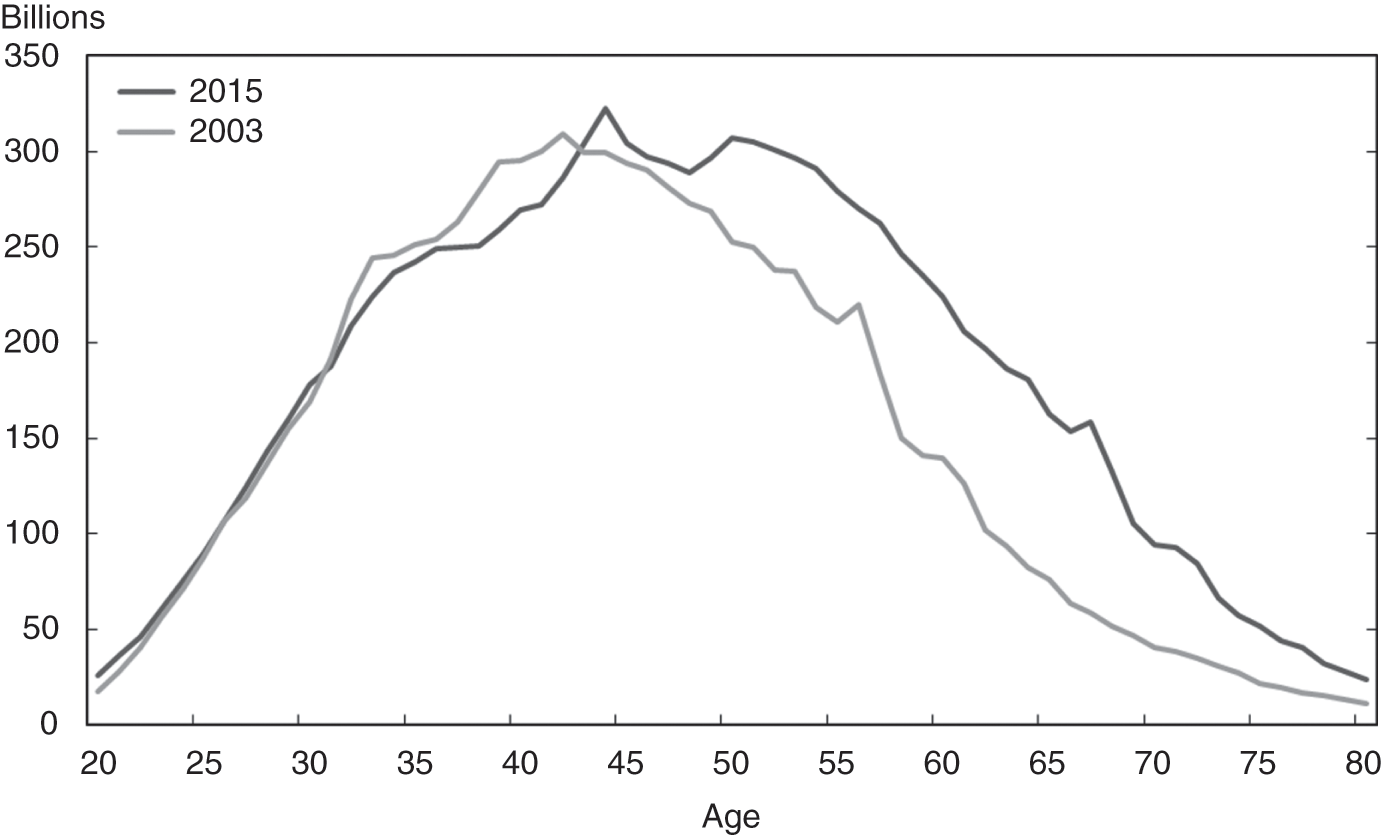
Figure 9.1 Total Debt Balance by Age of Borrower
The predominant factor driving increased debt was mortgages taken out in the 2000s; credit card debt actually fell over the same period for older households.6 This result is not surprising. After all, Greenspan and Kennedy (Reference Greenspan and Kennedy2005) pointed out that homeowners extracted $564 billion of home equity per year from 2001 to 2005.
Unfortunately, as debt is rising, most Americans of retirement age still have low balances of financial assets. According to the U.S. Census Bureau, median net worth excluding home equity in 2011 for the elderly aged 65 to 69 was only $43,921 (Figure 9.2).
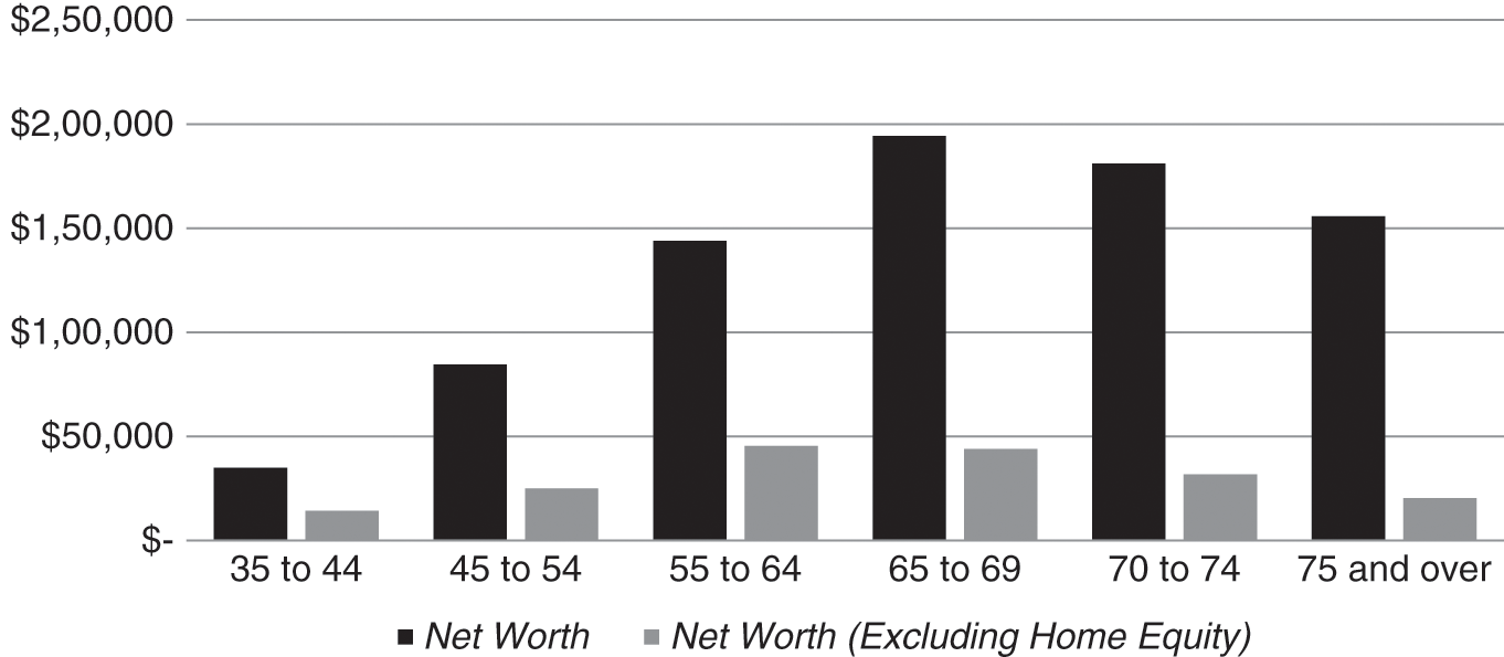
Figure 9.2 Median Net Worth in 2011
Thus it is not surprising that Poterba and colleagues (Reference Poterba, Venti and Wise2011) show that “Even if households used all of their financial assets … to purchase a life annuity, only 47 percent of households between the ages of 65 and 69 in 2008 could increase their life-contingent income by more than $5,000 per year.” Savings are not large enough at this point to address the growing needs of the elderly.
For older households struggling to finance retirement, owning a home may explain how many retirees are able to successfully get by.7 As shown in Figure 9.3, the share of elderly households owning their home increased by about five percentage points from 1982 to 2012 to a peak of nearly 84 percent of those aged 70 to 74. Since that time, the rate has fallen a bit (to 81 percent), but the vast majority of the elderly own their primary residence today. Owning a home can substantially reduce expenses and risk associated with retirement (Sinai and Souleles Reference Sinai and Souleles2005).
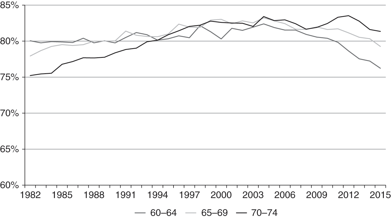
Figure 9.3 Homeownership Rate for Elderly Households, 60–74 Years Old
Homeowners appear more prepared for retirement than renters in almost every way. Census data show that median net worth including home equity is considerably larger than without (Figure 9.2) – almost $195,000 for households aged 65 to 69 in 2011. Poterba and colleagues (Reference Poterba, Venti and Wise2011) show that housing and real estate wealth exceeds the total of financial assets and personal retirement accounts for households of the same age. Even more striking, the authors show that real estate represents almost 80 percent of the present value of Social Security income.
In what follows, I examine the growth in mortgage debt and home equity for the elderly using the Survey of Consumer Finances (SCF) and consider how retirees are able to manage debt and utilize home equity in retirement with data from the Health and Retirement Survey (HRS). Previous academic research often examines home equity as a share of net worth without considering the amount of mortgage debt.8 Indebtedness is important to consider in its own right given the way many households now pay for their costs in retirement, predominantly financing expenditures from cash flow rather than spending down their stock of assets. As Poterba and colleagues (Reference Poterba, Venti and Wise2011) point out, the typical household appears to treat home equity and non-annuitized wealth like precautionary savings, which they spend only very late in life.
The data show a striking increase in mortgage debt at or near retirement age since 1992. For example, about 40 percent of households age 66–71 have a mortgage in 2013, up from 25 percent two decades earlier. At the same time, the average amount of mortgage debt (in 2013$) has almost tripled from less than $20,000 to more than $55,000. By contrast, real home equity in 2013 is at about the same level as it was almost 15 years earlier for most older homeowners. These data make clear that the growth of housing debt in the boom prior to the Great Recession remains on the balance sheets of many older households today.
Next I consider the evolution of mortgage debt versus financial assets over time. Debt is not necessarily a problem if homeowners have more assets to pay back the debt. Unfortunately, not only has debt increased as a share of home values, it has also increased relative to financial assets. About 40 percent of homeowners with a mortgage aged 65–69 had more mortgage debt than the sum total of all of their financial assets in 2012, up from about 28 percent in 1992.
Having established the growth in housing debt, I examine data from previous cohorts of older homeowners to examine how these households have historically managed mortgage debt and spent down home equity and financial assets over time. This analysis builds on a pair of papers by Poterba and colleagues (Reference Poterba, Venti, Wise and Wise2012, Reference Poterba, Venti and Wise2015) that examine the net worth of the elderly in the year just prior to death as well as examining the evolution of assets from retirement age to just before death.9
The evidence shows that few homeowners spend down home equity until very late in life. For a sample of borrowers first observed at age 53–63 in 1994 and who die within 18 years, the share without home equity increased slightly from 31 percent to 34 percent. For elderly first observed over age 70 in 1992 and who die within 15 years, the share without home equity doubled from 22 percent to 44 percent.10 Even for the oldest households in the sample, however, the majority own a home in the year prior to death.
Next I examine the link between home equity and financial assets. Poterba and colleagues (Reference Poterba, Venti and Wise2015) show that for households entering retirement with assets, most of those assets remain unspent unless the household has a disruption in family composition or a member with an important medical event. I expand on their analysis by separating assets into home equity and financial assets. The results show that most older households only spend down home equity in the years just prior to death when they enter assisted living. By contrast, households spend down 30 percent to 40 percent of financial assets. Homeowners with larger amounts of financial assets are slightly less likely to reduce home equity, potentially because they have the resources to age in place in their home rather than selling the home and moving to assisted living.
Putting these results together, my findings suggest that the prognosis for financial stability in retirement is getting worse because more households are entering retirement age with greater amounts of debt. This trend is likely to continue as younger cohorts are nearing retirement age with more debt than previous cohorts, whether measured in real dollars or as a share of home value (loan-to-value ratios are also rising). While many elderly have large amounts of home equity (which often exceeds other financial assets, including retirement accounts), most do not use that home equity to fund retirement.
This chapter has two empirical sections. The first examines the Survey of Consumer Finances to determine changes in household balance sheets and borrowing when heading into retirement. The second examines data from the Health and Retirement Survey to study how households spend down home equity and financial assets. This chapter concludes with ideas about a future policy and research agenda.
Housing Debt in Retirement
To begin, I examine data from the Survey of Consumer Finances to track homeownership and borrowing by families at or near retirement age. The analysis is conducted by age as well as by following cohorts of borrowers in six-year age intervals from 1992 to 2013. The six-year age intervals were designed to allow the reader to compare housing behavior of some cohorts.
Data Description
The Survey of Consumer Finances (SCF) is sponsored by the Federal Reserve Board in cooperation with the Department of Treasury. It is a cross-sectional survey of families in the United States that has taken place every three years since 1983. I start with the 1992 survey, which was the first date that the SCF was built to provide a nationally representative sample, using waves in 1992, 1995, 1998, 2001, 2004, 2007, 2010, and the latest published wave in 2013. The survey collects information on assets, liabilities, pensions, income, and demographics. About 6,500 families participate in each wave of the survey, which means that it can be difficult to separate into smaller groups of elderly without some sampling error. The yearly survey data were downloaded directly from the Federal Reserve website. Dollar-denominated variables are reported in 2013($) to allow comparisons across years. The primary variables used are X14 (age), X805 (balance still owed on first mortgage), X808 (mortgage payment), X701 (homeownership), X809 (payment frequency), X5729 (income), and X507 (value of primary residence). Sample weights (X4200) were applied throughout the data.
The term “family” is defined in the SCF by examining a household unit and dividing into a primary economic unit (PEU) – the family – and everyone else in the household (Board of Governors of the Federal Reserve System 2014). The PEU is intended to be the economically dominant single person or couple (whether married or living together as partners) and all other persons in the household who are financially interdependent with that economically dominant person or couple. In this regard, the definition of families in the SCF is more comparable to the definition of households in other government surveys.
The data are analyzed in four six-year age groups beginning in 1992 and based on the age of the head of the family: 54–59, 60–65, 66–71, and 72–77-year-olds. The cohorts were then aged every six years, the same intervals that align with years that cohorts are observed in the SCF. While the SCF takes place every three years, the data are aggregated into six-year age intervals to ensure a large enough sample for appropriate inferences. In the last year of study, the oldest cohort went from being 42–47 in 1992 to 72–77 years in 2013.
Analysis
To start, I examine changes in housing debt, homeownership, and home equity by age. Table 9.1 reports the share of families without a mortgage in the various age groups. Families with a mortgage in retirement may be at greater risk of losing their homes without working or obtaining additional income above and beyond Social Security.
Table 9.1: Percent of Households with No Mortgage by Age
| 1992 | 1995 | 1998 | 2001 | 2004 | 2007 | 2010 | 2013 | |
|---|---|---|---|---|---|---|---|---|
| 54–59 | 41% | 42% | 42% | 42% | 41% | 35% | 37% | 39% |
| 60–65 | 56% | 53% | 55% | 57% | 54% | 47% | 46% | 48% |
| 66–71 | 75% | 72% | 70% | 68% | 69% | 61% | 59% | 59% |
| 72–77 | 90% | 82% | 83% | 83% | 80% | 76% | 67% | 70% |
The data show a consistent downward trend in the share of homeowners with a paid-off home entering retirement age. For families whose head was over age 65 (in this case, age 66–71), the share without a mortgage fell from a high of 75 percent in 1992 to 69 percent in 2004, just prior to the financial crisis. By 2007, the percentage without a mortgage had fallen to 61 percent and remained around 59 percent in 2010 and 2013. Families with a head aged 72–77 years old exhibit a similar large decline in the share of borrowers without mortgages. Older borrowers appear to have strongly contributed to the growth in borrowing during the mid-2000s. By contrast, the share of borrowers aged 54 to 59 without a mortgage has remained relatively stable at between 35 percent and 42 percent. Thus the increase in debt appears to be a result of borrowers not paying off their mortgage as they approach and enter retirement age.
One possible explanation for the decline in the share of families with fully paid-off mortgages is that the homeownership rate was rising for older families during this same time period. As a result, some families who might have been renters in previous years became homeowners. Although these “new” homeowners may not have fully paid off their mortgage, they might have accumulated enough home equity to make retirement more financially stable than if they had not owned a home at all. Table 9.2, in fact, documents that the homeownership rate was rising over this time period for families whose head is age 66 and above.11
Table 9.2: Homeownership Rate by Age
| 1992 | 1995 | 1998 | 2001 | 2004 | 2007 | 2010 | 2013 | |
|---|---|---|---|---|---|---|---|---|
| 54–59 | 76% | 83% | 77% | 77% | 80% | 79% | 70% | 69% |
| 60–65 | 76% | 79% | 78% | 79% | 77% | 81% | 76% | 74% |
| 66–71 | 74% | 76% | 76% | 75% | 78% | 78% | 78% | 79% |
| 72–77 | 75% | 78% | 75% | 76% | 78% | 74% | 75% | 77% |
One way to address this issue is to examine the share of families with some housing payment.12 In this case, a homeowner with a mortgage might be treated similarly to a renter, at least from the perspective that both groups may require additional income relative to a homeowner with a fully paid-off mortgage. In fact, data from the Joint Center for Housing Studies of Harvard (2014) documents that about 30 percent of elderly households with a mortgage pay more than one-half of their income in housing expenses, a similar share as elderly renters. Thus mortgage payments could present an appreciable burden on elderly retirees just as rental payments might.
The data in Table 9.3 show that after 2007, a sharply higher share of families whose head is over the age of 65 fall into the category of owners with mortgage payment or renters. While in 2004, 47 percent of those aged 66 to 71 had some housing payment, by 2010 that number had risen to 54 percent. For the oldest families (with a head aged 72 to 77), the share rose from 38 percent to 50 percent. While the data in 2013 show a small decline in the share of elderly with a mortgage, the overall pattern documents that housing payments have become much more common among retirement-age families after the financial crisis.
Table 9.3: Percent with Housing Payments by Age
| 1992 | 1995 | 1998 | 2001 | 2004 | 2007 | 2010 | 2013 | |
|---|---|---|---|---|---|---|---|---|
| 54–59 | 69% | 65% | 67% | 67% | 67% | 72% | 74% | 73% |
| 60–65 | 57% | 58% | 57% | 55% | 58% | 62% | 65% | 64% |
| 66–71 | 44% | 45% | 47% | 49% | 47% | 52% | 54% | 53% |
| 72–77 | 33% | 36% | 38% | 37% | 38% | 44% | 50% | 45% |
Next, I examine the amount of mortgage debt held by families in this age group who own a home. Table 9.4 shows the average mortgage debt by age for homeowners with a mortgage and documents an appreciable rise over time in the amount of mortgage debt held by older borrowers.
Table 9.4: Real Mortgage Amount (2013$) by Age among Homeowners with a Mortgage
| 1992 | 1995 | 1998 | 2001 | 2004 | 2007 | 2010 | 2013 | |
|---|---|---|---|---|---|---|---|---|
| 54–59 | $ 32,610 | $ 39,559 | $ 44,860 | $ 52,574 | $ 62,471 | $ 68,561 | $ 67,174 | $ 69,954 |
| 60–65 | $ 23,118 | $ 28,023 | $ 43,512 | $ 47,562 | $ 63,578 | $ 69,082 | $ 69,099 | $ 71,418 |
| 66–71 | $ 18,304 | $ 23,342 | $ 31,997 | $ 40,180 | $ 43,219 | $ 66,052 | $ 54,790 | $ 54,828 |
| 72–77 | $ 16,419 | $ 23,359 | $ 34,113 | $ 34,662 | $ 47,338 | $ 36,677 | $ 46,892 | $ 40,360 |
Overall real mortgage debt among 66–71-year-olds increased from about $18,000 in 1992 (in 2013 dollars) to about $55,000 in 2010 and 2013. This is a sharp growth in borrowing for an age group that is at or near retirement. At first glance, it is surprising that the amount of borrowing grew throughout the 1990s and early 2000s, in seeming contradiction of the Greenspan and Kennedy (Reference Greenspan and Kennedy2005) result showing a much sharper increase in mortgage borrowing in the early 2000s than the 1990s. However, the data on the share of homeowners with a mortgage can reconcile this seeming contradiction. Table 9.3 shows that the share of families without a mortgage fell from 2001 to 2007. This suggests that the mortgage excesses of the 2000s resulted in increases in mortgage debt on both the intensive and extensive margins; not only did borrowers take on more housing debt, but a larger share of older borrowers had a mortgage than in previous years.
Of course, families may have seen an increase in home values that offset the larger overall borrowing amounts. Table 9.5 reports loan-to-value (LTV) ratios for the same age groups, once again conditioned on having an outstanding mortgage.13 While mortgage debt grew steadily prior to 2007, the overall LTVs for these age groups only increased slightly between 1998 and 2007. This suggests that the typical family increased its borrowing roughly in proportion with the overall rise in home prices. However, after the housing crash, LTVs exhibited a large increase. By 2013, the typical older borrower over age 65 had an LTV of almost 50 percent, up more than 10 percentage points from 1998. The data suggest that mortgage debt for older families increased when home values rose, but that borrowers did not decrease their mortgage debt when prices fell.
Table 9.5: Mean Loan-to-Value (LTV) Ratio among Homeowners with a Mortgage
| 1992 | 1995 | 1998 | 2001 | 2004 | 2007 | 2010 | 2013 | |
|---|---|---|---|---|---|---|---|---|
| 54–59 | 32% | 40% | 43% | 43% | 43% | 42% | 56% | 59% |
| 60–65 | 29% | 36% | 37% | 43% | 39% | 40% | 52% | 58% |
| 66–71 | 22% | 33% | 34% | 36% | 38% | 41% | 50% | 48% |
| 72–77 | 17% | 32% | 37% | 37% | 43% | 40% | 41% | 49% |
While the SCF data from 2016 are not yet available, it is possible that the trend of increasing LTVs might reverse itself. Between 2013 and 2016, home values have risen about 20 percent according to the Case and Shiller National Home Value Index.14 Thus LTVs today would be close to their historical average of 40 percent as long as mortgage balances have not gone up for elderly borrowers, which would be consistent with data showing the overall size of mortgage borrowing has been flat over this time period.15
Finally, I examine overall home equity. Table 9.6 reports home equity in real 2013 dollars for all families who own a home. Not surprisingly, given the data on LTVs, home equity has been relatively stable around $100,000 since the early 2000s for families aged 66–71, with the exception of a large increase in 2007 followed by a decline in 2010.16 This is consistent with studies finding that owners have large amounts of home equity, even those older homeowners with a mortgage.
Table 9.6: Home Equity (Real 2013$) among All Homeowners
| 1992 | 1995 | 1998 | 2001 | 2004 | 2007 | 2010 | 2013 | |
|---|---|---|---|---|---|---|---|---|
| 54–59 | $ 101,904 | $ 98,258 | $ 104,718 | $ 123,660 | $ 145,815 | $ 162,934 | $ 120,013 | $ 119,124 |
| 60–65 | $ 80,939 | $ 77,683 | $ 117,603 | $ 109,922 | $ 163,279 | $ 170,605 | $ 133,546 | $ 122,818 |
| 66–71 | $ 83,006 | $ 70,088 | $ 94,357 | $ 110,136 | $ 114,036 | $ 162,783 | $ 109,641 | $ 114,094 |
| 72–77 | $ 97,417 | $ 73,644 | $ 92,530 | $ 93,666 | $ 110,457 | $ 92,719 | $ 114,158 | $ 82,193 |
The data from this section show that a growing number of families are entering retirement age with mortgage debt that will not be paid off for many years to come. The increasing amounts of mortgage debt will likely challenge retirement stability for some homeowners.
Spending Home Equity and Financial Assets in Retirement
Next, I turn to the questions of how mortgage debt has evolved relative to assets for older homeowners, as well as how these homeowners spend down their assets in retirement. Here, this chapter uses information in the Health and Retirement Survey (HRS), following closely the analysis in Poterba and colleagues (Reference Poterba, Venti and Wise2015). These authors take advantage of the panel feature of the HRS to identify assets in the last wave prior to death and compare them to assets that the same household had when it first entered the HRS up to 20 years earlier. The point of the analysis is to understand how households spend down assets, including both housing and other financial assets in typical retirement years. An important advantage of the HRS for this analysis is the opportunity to observe a large sample of respondents in the very late stages of life.
Data Description
The University of Michigan Health and Retirement Study is a nationally representative survey of Americans over the age of 50. The survey has interviewed a sample of approximately 20,000 individuals every two years since its inception in 1992. Eleven waves of the study are included in this dataset.
Two of the six age cohorts of the HRS are included in our dataset. They are the base HRS cohort and the AHEAD cohort. The HRS cohort includes individuals born from 1931 to 1941 and are ages 51 to 61 in 1992. The AHEAD cohort began as part of a different study (The Study of Assets and Health Dynamics among the Oldest Old) in 1993 and includes individuals born before 1924. The AHEAD cohort was interviewed once more in 1995 before being added to the general HRS interview for the 1998 study. For the purposes of this study, the 1993 AHEAD cohort responses are added to the 1994 HRS study responses (wave 2) and the 1995 AHEAD cohort responses are added to the 1996 HRS study responses (wave 3). I drop the first wave of the HRS (1992 sample) due to data problems, so the sample begins with wave 2. The data file used is the RAND HRS Data (Version O) file. The RAND HRS Data file is a cleaned version with derived variables of all the core interviews of all waves of the HRS. All data are listed under the respondent level, but wealth variables are collected on the household level and can be identified through a household ID (HHID).
As I am predominantly interested in assets at end of life, responses for this study are limited only to respondents who died during the survey time period (after 1993 and prior to 2012). The data choices that follow closely track those in Poterba and colleagues (Reference Poterba, Venti and Wise2015). Respondents with spouses who are not eligible for the HRS due to their age, and any respondents who left for reasons other than death are also dropped. When looking at the change in assets up to the year prior to death, the analysis is limited to respondents who joined the study at the beginning (i.e., 1994 for HRS and 1993 for AHEAD). This includes the majority of respondents from these years (wave 2). Variables indicating which survey year the respondent enters the survey (FYO – First Year Observed) and when the respondent last fully completes the survey (LYO – Last Year Observed) are created. The LYO variable can range from only a few months to two years before the time the respondent dies. On average, given that the HRS is conducted every two years, the LYO is about a year before death. The HRS provides separate codes for respondents who exit the sample due to death versus attrition; I consider only those who died in determining LYO.
Wealth assets are computed in multiple categories and converted into 2012 dollars using the Consumer Price Index. Housing wealth comes from housing equity (home value net of mortgage debt). Other wealth is made up of non-housing real estate equity, vehicles, business, and second home equity minus other debt. Annuity wealth includes both the respondent’s and their spouse’s pension and Social Security wealth. Financial wealth is made up of IRA accounts, stocks, checking accounts, CDs, bonds, and other financial assets.
Health variables for specific conditions are dummies that indicate whether a condition appears from the FYO to the LYO. The general health variable is a percentile index created as described in Poterba and colleagues (Reference Poterba, Venti and Wise2013) with a range from one to 100, with one being the lowest. For all health conditions and dummies, the value is made positive if either the respondent or their spouse reports the issue. This way, the respondent-level health data more closely resemble the household-level wealth data.
Education variables are constructed by years of education. Family pathway variables are constructed using the marriage status variable. The family pathways indicate whether the respondent stays single, stays married, or goes from married to single. There were too few responses for single to married to be included in the study.
Analysis
To start, I examine additional metrics describing the ability of borrowers to retire their mortgage. Figure 9.4 uses all waves of the HRS starting in 1998 along with sample weights to compare the amount of mortgage debt relative to financial assets. The goal is to determine whether households have enough financial assets to pay off their mortgages if they chose to do so. In 1998, only 25 percent of those with a mortgage had a larger mortgage balance than financial assets. In other words, about three-quarters of mortgage borrowers could retire their mortgage if they chose to do so.17 However, the share unable to retire their mortgage has been steadily increasing, up to 40 percent in 2012.
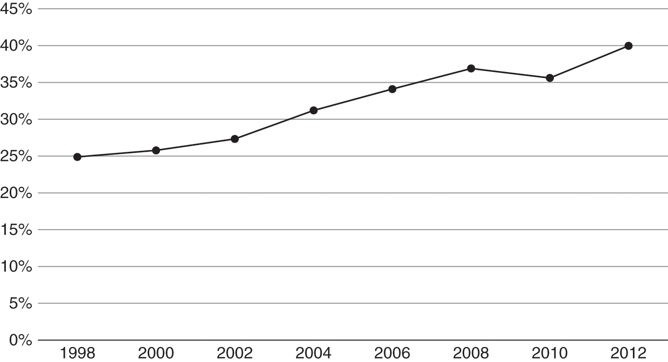
Figure 9.4 Percent of Homeowners with a Mortgage Aged 60–69 with More Mortgage Debt than Financial Assets
Another way to consider the burden associated with carrying a mortgage is to examine the extent to which borrowers who start with a mortgage end up paying it off before passing away. To do this, Table 9.7 reports data on mortgage amounts for all households in first and last year observed for the AHEAD and HRS samples. The data suggest that the bulk of borrowers who start retirement age with a mortgage do not fully pay it off by the time of their death. Among the younger HRS borrowers who enter the sample at ages 53 to 63 in 1994, the share with a mortgage increases from 62.5 percent to 71.8 percent. In other words, of the 37.5 percent with a mortgage, only about one-quarter of households (9.3 percent) pay off their mortgage up to the year prior to death. Not surprisingly, the bulk of those that pay off the mortgage appear to be borrowers with mortgage debt under $50,000 in 1994. In the AHEAD group of borrowers entering the sample at age 70 and above, a much higher share of borrowers start the sample without debt (89 percent) and more than 40 percent of the remainder pay off their mortgage prior to death. In both cohorts, however, most borrowers who enter retirement age with a mortgage will have at least some mortgage payments up to the year prior to passing away.
Table 9.7: Mortgage Debt
| HRS | AHEAD | |||
|---|---|---|---|---|
| First Year Observed | Last Year Prior to Death | First Year Observed | Last Year Prior to Death | |
| < = 0 | 62.5% | 71.8% | 89.0% | 93.4% |
| $1–$50k | 19.7% | 11.3% | 2.4% | 1.2% |
| $50,001–$100k | 8.7% | 9.0% | 5.1% | 2.7% |
| $100,001–$250k | 7.8% | 6.8% | 2.2% | 1.5% |
| $250,001–$500k | 1.2% | 1.1% | 1.2% | 1.1% |
| > 500k | 0.1% | 0.0% | 0.1% | 0.2% |
| Total | 100.0% | 100.0% | 100.0% | 100.0% |
HRS Sample: Respondents age 51–61 in 1992 who died prior to 2012
AHEAD Sample: Respondents age 70+ in 1993 who died prior to 2012
Next, I examine the amount of home equity and compare it to financial assets. The goal is to examine whether the type of asset is related to the likelihood that a household liquidates the asset over time to help fund retirement. Tables 9.8 and 9.9 compare the distribution of home equity and financial assets for those in the HRS sample (age 53–63 in 1994) and the AHEAD sample (over age 70 in 1993).
Home Equity vs. Financial Assets, AHEAD Sample (respondents aged 70+ in 1993 who died prior to 2012).
Panel 1. Responses in 1993
| Total Financial Assets | |||||||||
|---|---|---|---|---|---|---|---|---|---|
| < = 0 | $1–$10k | $10,001–$50k | $50,001–$100k | $100,001–$250k | $250,001–$500k | >500k | Total Financial | ||
| < = 0 | 6.2% | 5.0% | 6.1% | 1.5% | 1.9% | 0.9% | 0.6% | 22.2% | |
| $1–$10k | 0.5% | 0.4% | 0.9% | 0.0% | 0.1% | 0.0% | 0.0% | 1.9% | |
| Total | $10,001–$50k | 2.4% | 2.2% | 4.5% | 1.2% | 1.3% | 0.6% | 0.2% | 12.4% |
| Home | $50,001–$100k | 2.2% | 2.1% | 7.5% | 3.2% | 4.2% | 2.6% | 1.2% | 23.0% |
| Equity | $100,001–$250k | 1.9% | 1.9% | 5.6% | 4.8% | 8.1% | 5.0% | 4.2% | 31.5% |
| $250,001–$500k | 0.2% | 0.2% | 0.8% | 0.9% | 2.0% | 1.2% | 1.9% | 7.2% | |
| > 500k | 0.0% | 0.0% | 0.5% | 0.0% | 0.1% | 0.2% | 1.1% | 1.9% | |
| Total Home | 13.4% | 11.8% | 25.9% | 11.6% | 17.7% | 10.5% | 9.2% | 100.0% | |
Note: All data reported in $2012; N = 5,581
22.9 percent of respondents have less than 50k in financial wealth and more than 50k in home equity
8.3 percent of respondents have less than 50k in home equity and more than 50k in financial assets
Panel 2. Responses in Last Year in Sample Prior to Death
| Total Financial Assets | |||||||||
|---|---|---|---|---|---|---|---|---|---|
| < = 0 | $1–$10k | $10,001–$50k | $50,001–$100k | $100,001–$250k | $250,001–$500k | >500k | Total Financial | ||
| < = 0 | 12.7% | 10.8% | 8.4% | 3.2% | 4.1% | 2.2% | 2.3% | 43.7% | |
| $1–$10k | 0.4% | 0.4% | 0.5% | 0.1% | 0.1% | 0.0% | 0.0% | 1.5% | |
| Total | $10,001–$50k | 1.9% | 2.1% | 3.2% | 1.1% | 0.9% | 0.4% | 0.4% | 10.0% |
| Home | $50,001–$100k | 1.7% | 2.6% | 4.5% | 2.3% | 2.8% | 1.4% | 1.3% | 16.6% |
| Equity | $100,001–$250k | 1.0% | 1.6% | 4.0% | 2.9% | 5.0% | 3.2% | 3.3% | 21.0% |
| $250,001–$500k | 0.2% | 0.4% | 0.6% | 0.8% | 1.1% | 0.8% | 1.7% | 5.6% | |
| > 500k | 0.0% | 0.1% | 0.1% | 0.1% | 0.2% | 0.2% | 1.2% | 1.9% | |
| Total Home | 17.9% | 18.0% | 21.3% | 10.5% | 14.2% | 8.2% | 10.2% | 100.0% | |
Note: All data reported in $2012; N = 5,581
16.80 percent of respondents have less than 50k in financial wealth and more than 50k in home equity
14.80 percent of respondents have less than 50k in home equity and more than 50k in financial assets
Home Equity vs. Financial Assets, HRS Sample (respondents aged 53–63 in 1994 who died prior to 2012).
Panel 1. Responses in 1994
| Total Financial Assets | |||||||||
|---|---|---|---|---|---|---|---|---|---|
| < = 0 | $1–$10k | $10,001–$50k | $50,001–$100k | $100,001–$250k | $250,001–$500k | >500k | Total Financial | ||
| < = 0 | 15.2% | 6.5% | 4.9% | 1.0% | 1.7% | 1.0% | 0.4% | 30.7% | |
| $1–$10k | 1.3% | 0.7% | 0.7% | 0.2% | 0.2% | 0.0% | 0.0% | 3.1% | |
| Total | $10,001–$50k | 4.7% | 3.9% | 4.8% | 1.9% | 1.9% | 0.6% | 0.4% | 18.2% |
| Home | $50,001–$100k | 3.7% | 3.5% | 5.7% | 2.8% | 3.1% | 1.3% | 0.7% | 20.8% |
| Equity | $100,001–$250k | 1.3% | 1.5% | 3.4% | 2.6% | 6.0% | 3.6% | 3.5% | 21.9% |
| $250,001–$500k | 0.1% | 0.1% | 0.3% | 0.6% | 1.2% | 0.9% | 1.2% | 4.4% | |
| > 500k | 0.0% | 0.0% | 0.0% | 0.0% | 0.0% | 0.0% | 0.7% | 0.7% | |
| Total Home | 26.3% | 16.2% | 19.8% | 9.1% | 14.1% | 7.4% | 6.9% | 100.0% | |
Note: All data reported in $2012
N = 2,154
19.6 percent of respondents have less than 50k in financial wealth and more than 50k in home equity
9.3 percent of respondents have less than 50k in home equity and more than 50k in financial assets
Panel 2. Responses in Last Year in Sample Prior to Death
| Total Financial Assets | |||||||||
|---|---|---|---|---|---|---|---|---|---|
| < = 0 | $1–$10k | $10,001–$50k | $50,001–$100k | $100,001–$250k | $250,001–$500k | > 500k | Total Financial | ||
| < = 0 | 15.5% | 8.3% | 6.0% | 1.1% | 1.6% | 0.6% | 0.5% | 33.6% | |
| $1–$10k | 0.6% | 0.6% | 0.8% | 0.0% | 0.1% | 0.0% | 0.0% | 2.1% | |
| Total | $10,001–$50k | 4.1% | 3.0% | 4.7% | 1.5% | 1.4% | 0.8% | 0.2% | 15.7% |
| Home | $50,001–$100k | 2.6% | 2.1% | 5.2% | 2.7% | 3.0% | 1.1% | 0.7% | 17.4% |
| Equity | $100,001–$250k | 1.5% | 1.6% | 3.9% | 3.2% | 4.6% | 2.8% | 3.8% | 21.4% |
| $250,001–$500k | 0.3% | 0.1% | 0.8% | 1.0% | 1.4% | 1.3% | 2.2% | 7.1% | |
| > 500k | 0.0% | 0.0% | 0.1% | 0.1% | 0.4% | 0.0% | 1.8% | 2.4% | |
| Total Home | 24.6% | 15.7% | 21.5% | 9.6% | 12.5% | 6.6% | 9.2% | 100.0% | |
Note: All data reported in $2012; N= 2,154
18.20 percent of respondents have less than 50k in financial wealth and more than 50k in home equity
7.80 percent of respondents have less than 50k in home equity and more than 50k in financial assets
First consider the older AHEAD respondents. Panel 1 in Table 9.8 shows that households over age 70 in 1993 held significant amounts of home equity; on average 48 percent had more than $100,000 ($2012) and another 23 percent had more than $50,000.18 In fact, housing wealth represents the bulk of wealth for households. Almost 23 percent of respondents had more than $50,000 in home equity and less than $50,000 in financial assets, whereas only 8.3 percent had the opposite – more than $50,000 in financial assets and less than $50,000 in home equity. Alternatively, about 44 percent of respondents had home equity that was at least one category higher than financial assets, whereas 39 percent had at least one more category of financial assets. At the top end of the wealth distribution, there is an appreciable proportion of households (17 percent) that have more than $250,000 in financial assets, but less in home equity. Thus for the elderly with high net worth, housing is less important as a share of total assets, whereas at the lower end of the wealth distribution, home equity is much more important.
Of particular interest with the HRS (and AHEAD sample) is the ability to look at respondents just prior to death at much older ages than would be possible with other data. Panel 2 in Table 9.8 shows the same comparison of home equity and financial assets in the last wave observed prior to death.
One striking feature is the sharp increase in households who appear to have liquidated their home and own no home equity. More than 43 percent of respondents report having no home equity versus 22 percent in the first year surveyed (1993) from Panel 1. As well, another 15 percent of respondents report having less than $50,000 in home equity and more than $50,000 in financial assets. Overall, almost one-half now report having at least one more bucket of financial assets relative to home equity (26.5 percent have at least one category more of home equity).
It is also striking just how many respondents hit the last stage of their life having completely exhausted their financial assets (a point first made by Poterba et al. Reference Poterba, Venti, Wise and Wise2012). Almost 36 percent have less than $10,000 in financial assets and another 21 percent have less than $50,000 in financial assets. Two-thirds of those with less than $10,000 of financial assets (23.5 percent) also have no home equity. These households are ill-prepared to fund unreimbursed medical expenses and other costs. Many of these elderly will end up on Medicaid in addition to Medicare, with the government funding all of the costs associated with the last stages of their lives.19
Table 9.9 repeats this same analysis using younger households in the HRS sample (age 53–63 in 1994). The HRS respondents appear to head into retirement age in similar circumstances as AHEAD households (Panel 1). The younger HRS respondents with low net worth still hold portfolios disproportionately concentrated in home equity, whereas the respondents with higher net worth have a more balanced portfolio. Almost 20 percent have more than $50,000 ($2012) in home equity and less than $50,000 in financial assets, whereas only 9 percent have the reverse situation. However, unlike their older AHEAD counterparts, few HRS respondents have liquidated their housing equity in the year prior to death. In their last year observed, about two-thirds still own their home. About 18 percent have more than $50,000 ($2012) in home equity and less than $50,000 in financial assets, versus less than 8 percent in the reverse situation. And nearly 32 percent have at least one category more in home equity than financial assets as in Table 9.9. The comparison with the AHEAD cohort seems to suggest that households do not spend down home equity until they reach much older ages. The oldest respondents in the HRS sample would have died by age 81, whereas the AHEAD cohort has been observed into much older ages.20
To better understand how households spend housing and financial wealth as they age, I examine the determinants of assets in the last year observed as a function of assets when households are first surveyed plus demographic and health controls. The regressions in Table 9.10 follow the same format and include the same control variables as in Poterba and colleagues (Reference Poterba, Venti and Wise2015), tables 3.1 and 3.2.21 However, I make two adjustments. First, the regressions address skewness in observed wealth data by removing the top and bottom 3 percent of the dependent variable. Trimming the data results in more consistent estimates in the following regressions, although the overall findings are little changed. Second, I decompose assets in the form of home equity and financial wealth. The goal is to determine whether the type of asset has an impact on the likelihood that a household liquidates that asset to pay for expenses in retirement. Given that home equity is much less liquid than financial assets, it would not be surprising that households spend down these assets at different rates.22
Determinants of Assets in Last Year Observed, HRS Sample (respondents aged 53–63 in 1994 who died prior to 2012); AHEAD Sample (respondents aged 70+ in 1993 who died prior to 2012)
Panel 1. Regression of Net Worth in Last Year Observed
| Dependent Variable: Net Worth – Last Year Observed | ||||
|---|---|---|---|---|
| (1) HRS | (2) HRS | (3) AHEAD | (4) AHEAD | |
| Net Worth – First Year Observed | 1.078*** | 1.022*** | 1.058*** | 1.005*** |
| Health Controls | N | Y | N | Y |
| Demographics | N | Y | N | Y |
| Household Type Controls | N | Y | N | Y |
| Time between First/Last Observed | N | Y | N | Y |
| Constant | 37946.0*** | −35902.7 | 22452.0*** | −5994.8 |
| Number of Observations | 1414 | 1414 | 2526 | 2526 |
| R-Squared | 0.676 | 0.690 | 0.674 | 0.683 |
* p < 0.05, ** p < 0.01, *** p < 0.001
Panel 2. Regression of Home Equity in Last Year Observed, Separate Controls for Home Equity and Financial Assets
| Dependent Variable: Home Equity – Last Year Observed | ||||
|---|---|---|---|---|
| (1) HRS | (2) HRS | (3) AHEAD | (4) AHEAD | |
| Home Equity – First Year Observed | 0.69*** | 0.614*** | 0.81*** | 0.78*** |
| (29.30) | (25.16) | (53.58) | (50.49) | |
| Financial Assets – First Year Observed | 0.083*** | 0.077*** | 0.021*** | 0.016*** |
| (18.08) | (17.22) | (5.15) | (3.84) | |
| Health Controls | N | Y | N | Y |
| Demographics | N | Y | N | Y |
| Household Type Controls | N | Y | N | Y |
| Time between First/Last Observed | N | Y | N | Y |
| Constant | 27853*** | –25029.9** | 3022 | –1635 |
| Number of Observations | 1414 | 1414 | 2526 | 2526 |
| R-Squared | 0.578 | 0.617 | 0.575 | 0.592 |
* p < 0.05, ** p < 0.01, *** p < 0.001
Panel 3. Regression of Financial Assets in Last Year Observed, Separate Controls for Home Equity and Financial Assets
| Dependent Variable: Financial Assets – Last Year Observed | ||||
|---|---|---|---|---|
| (1) HRS | (2) HRS | (3) AHEAD | (4) AHEAD | |
| Home Equity – First Year Observed | 0.39*** | 0.31*** | 0.57*** | 0.53*** |
| (8.04) | (6.09) | (21.00) | (19.38) | |
| Financial Assets – First Year Observed | 0.77*** | 0.74*** | 0.64*** | 0.62*** |
| (37.97) | (35.04) | (47.71) | (43.81) | |
| Health Controls | N | Y | N | Y |
| Demographics | N | Y | N | Y |
| Household Type Controls | N | Y | N | Y |
| Time between First/Last Observed | N | Y | N | Y |
| Constant | 11632** | –47736.5** | –2830 | –51074.9*** |
| Number of Observations | 1414 | 1414 | 2526 | 2526 |
| R-Squared | 0.614 | 0.63 | 0.608 | 0.618 |
* p < 0.05, ** p < 0.01, *** p < 0.001
The results in the basic regression in Panel 1 of Table 9.10 are surprising at first blush – household assets in the last year observed are very similar to or slightly larger than assets in the first year observed. In other words, households do not appear to spend down assets, even by the year prior to death. These results remain whether looking at the younger HRS sample or the older AHEAD cohort, with coefficients on beginning of sample assets between 1.02 and 1.08. In Panel 1, and in the remaining two panels, the R-squared increases modestly with the inclusion of time between first and last year observed, as well as demographic, health, and household type variables. Many of these control variables are statistically significantly different from zero with the expected sign. However, the inclusion of these control variables does not change the interpretation of the regressions, although it slightly reduces the size and significance of the coefficient on beginning of sample asset balances.
The next two panels present separate regressions using a dependent variable for first year observed home equity (Panel 2) and financial assets (Panel 3). These results suggest it is important to examine the type of asset when considering changes in asset balances over time.
The home equity regressions show that respondents decrease home equity from the beginning of sample values, as we found in Tables 9.8 and 9.9, with coefficient estimates around 0.65 (HRS) and 0.8 (AHEAD). However, the extent to which the elderly reduce home equity does not appear to depend nearly as much on first-year observed financial assets, with coefficients of only 0.08 (HRS) to 0.02 (AHEAD). All of these coefficients are strongly statistically different than zero.
To better understand these findings, I examine where households live if they have no home equity in the year prior to life. More than two-thirds of borrowers with no home equity are living in a nursing home or assisted living in the last year observed. Thus, rather than selling the home to utilize the assets to support the costs of retirement, most people appear to sell their home as a result of a health care event. The fact that the coefficient on home equity prior to death is well below 1.0 seems to be predominantly a function of when or if a household moves into assisted living. In fact, most households remain homeowners throughout their lives and do not access their housing wealth prior to death. The fact that home equity is partly related to financial assets might be explained by wealthier households having resources to live longer at home.
By contrast, the last year observed financial assets in Panel 4 is highly correlated with the first year observed home equity, with coefficients of about 0.35 (HRS) to approximately 0.55 (AHEAD). This result appears consistent with those in Panel 2. After all, if most homeowners sell their home due to a medical event and move into assisted living, the remaining home equity would be converted into financial assets when the home is sold. This interpretation is consistent with the coefficient on home equity being larger for the AHEAD sample, as the oldest households are more likely to sell a home and move into assisted living.
The pattern of spending down beginning of period financial assets, by contrast, shows an opposite pattern with coefficients around 0.75 (HRS) and 0.6 (AHEAD). Again, it is not surprising that older households spend down financial assets more quickly than younger households. Younger households who die may do so unexpectedly early and thus be left with more assets, whereas older households may be more willing to spend down assets. Nonetheless, households have more than one-half of their first year observed assets in the year prior to death.
Decomposing asset types shows that the mix of assets is an important determinant of the extent to which a household spends assets later in life. While the initial regression that combines assets together suggests that there is little spend down of wealth by the elderly, separating the behavior of housing assets and financial assets gives a much more nuanced view. Households have a much greater propensity to spend financial assets, but not housing wealth.
Conclusion
The relationship between housing wealth, mortgages, and retirement readiness is taking on increasing importance as many more households enter retirement age without defined benefit retirement accounts and are thus reliant on assets to support their lifestyle. Home equity is the largest asset for the vast majority of retirement-age households. According to the U.S. Census, in 2011, median net worth including home equity for 65–69-year-olds was $194,000, whereas median net worth without home equity was only $44,000.
This chapter presents some new evidence to better understand the challenges facing near retirees. First, this chapter separately examines changes over time in the movement of mortgage debt, homeownership, and home equity. Often in previous research, the existence of growing mortgage debt is hidden in computations of home equity, which has remained roughly steady over the past 15 years, even as real home prices have risen. Second, I reexamine how households spend down assets up to the year prior to death, separately analyzing home equity and financial assets rather than combining them into a single measure of net worth.
For households with a head aged 66 to 71 and thus of traditional retirement age, the results suggest twin challenges – a large increase in mortgage debt at the same time that more households are paying a mortgage. Real mortgage debt ($2012) rose from $18,000 in 1992 to almost $55,000 in 2013 in this age group. At the same time, the share of households with a mortgage has risen from 25 percent to 41 percent. The combined effect is that more households face a larger debt burden. However, real home equity has remained roughly flat since 2001 at about $110,000, although it is up about $30,000 since 1992. Loan-to-value ratios are up from 22 percent to 48 percent. By any measure, older homeowners today are facing more financial challenges than in previous decades.
Historically, retiring without mortgage debt has been key to financial stability. Homeowners older than age 65 who are paying off a mortgage appear nearly as financially constrained as renters. The Joint Center for Housing Studies of Harvard (2014) reports that 30 percent of owners with a mortgage pay more than one-half of their income in housing costs, leaving few resources available to cover other basic expenses and health care. Similarly, about 30 percent of all older renters pay 50 percent of more of their income in housing expenses.23
A second question is whether homeowners can leverage existing home equity or financial assets to help cover their mortgage or other retirement expenses. Here I examine past behavior of elderly homeowners.
The data show, historically speaking, that most households entering retirement age with a mortgage do not fully retire the mortgage debt in retirement. In fact, only about 25 percent to 35 percent of older homeowners with a mortgage in 1992 had paid off their mortgage by the year prior to death. As well, the bulk of homeowners entering retirement age do not appear to spend down home equity, except when they move out of their home to enter assisted living. The elderly appear more willing to spend financial assets while living independently, although households have more than one-half of financial assets remaining in the year prior to death. Unfortunately, about 40 percent of all homeowners with a mortgage have more mortgage debt than financial assets.
In response to these challenges, many households report that they will work longer. The Federal Reserve 2015 Survey of Household Economics and Decisionmaking reports that more than one-half of respondents expect to either retire after age 65 or to never retire.24 The plan to work longer is a recent phenomenon and appears to be driven more by financial necessity than a longer life expectancy. The Employee Benefit Research Institute (Helman et al. Reference Helman, Copeland and VanDerhei2015) has been surveying individuals for 25 years about their retirement preparedness and expectations. The share of respondents stating that they expected to work after age 65 has grown from 11 percent in 1991 to 23 percent in 2000, to 46 percent by 2015.25 See Figure 9.5.
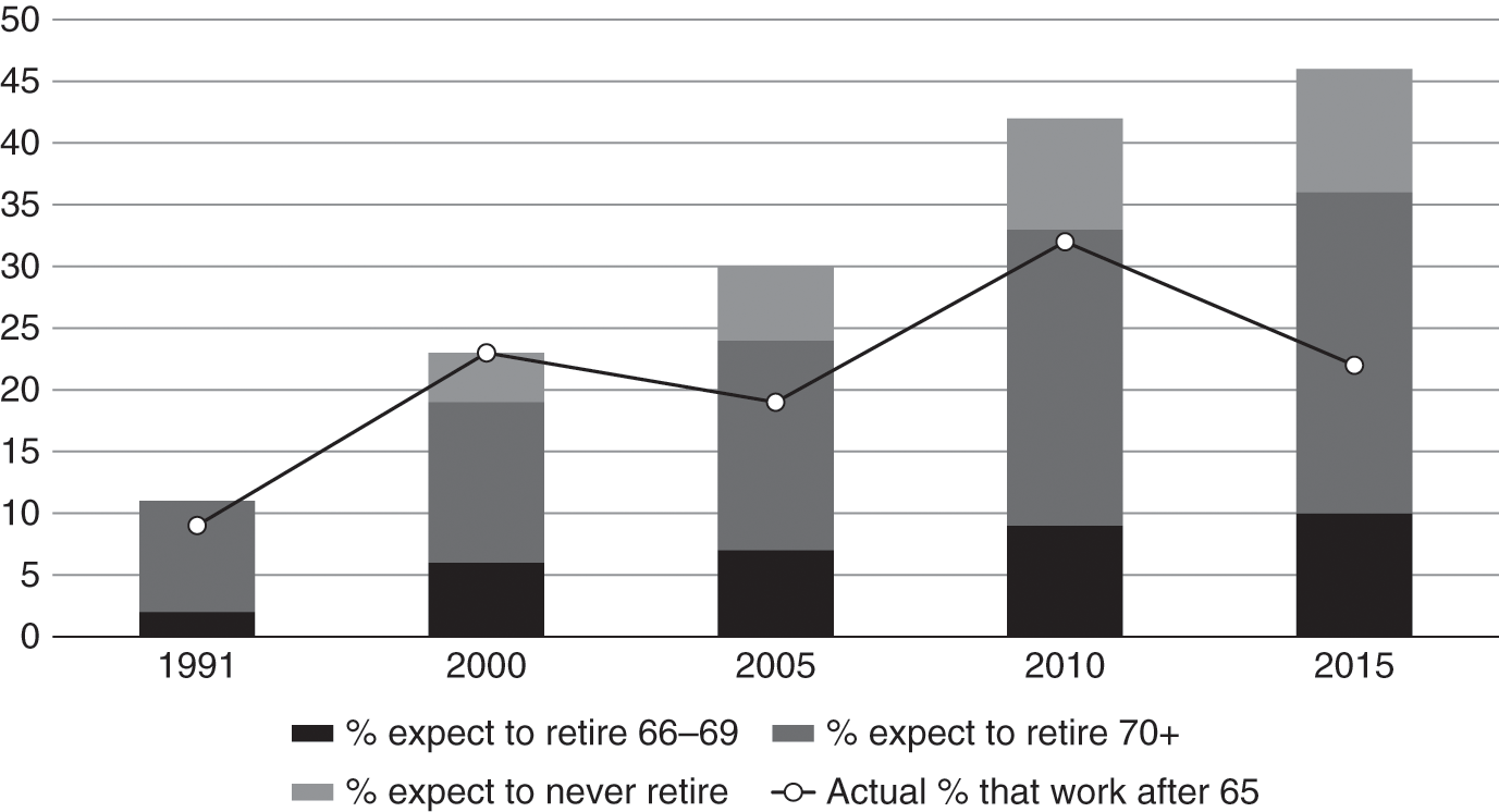
Figure 9.5 Late Retirement Expectations vs. Actual Retirement Age
Similarly, the EBRI data point out that borrowers who have debt or lack a retirement plan are much less confident in their ability to have enough money to fund retirement.
The problem with working longer, however, is that it may not be feasible for many of the elderly, either due to health problems or the inability to keep or obtain a job, especially for the middle-income or low-income households that this study shows have the largest increase in housing debt. In the EBRI survey, the share of people actually working after age 65 (22 percent) is about one-half as large as the share who say they intend to work after age 65 (46 percent).26 This is a striking change from 15 years ago, when worker expectations about working longer seemed to match the reality in the data. A recent Pew study27 showed that 19 percent of people aged 65 and above are working full- or part-time, up from 13 percent in 2000. This share of the elderly who are working has grown steadily, but the largest increases are in high-income professions like management, sales, and legal, whereas three of the four largest declines are in low-paid professions like food preparation, construction, and production.
Despite these apparent challenges, the elderly poverty rate remains near record lows, so many elderly are getting by with what they have. Of course, the traditional measurement of poverty does not consider asset or debt balances, and the measurement of health care expenses is difficult. Future research should examine the implications of growing debt in retirement and how households manage home equity. How are households paying this debt? Will poverty rates continue to grow? And how do these trends impact taxpayers? Are indebted households more likely to tap Medicaid to pay for at home or nursing home care?
Policy makers and business leaders have proposed a number of solutions to address these challenges. Some propose reform in the type of advice given to workers, the cost of delivering retirement products, and/or the creation of greater incentives for workers to save. Others suggest the development of new or more cost-effective financial products to tap home equity without selling the home28 or to annuitize existing savings. Nonetheless, the results in this chapter suggest something will need to change in order for many older Americans to have a more comfortable and satisfying retirement.
Author’s Note
The opinions, analysis, and conclusions of this chapter are those of the author. Monica Clodius provided excellent research assistance. This chapter benefited from the help of Jim Poterba and Steve Venti, who shared programs and insights from their previous analysis of the Health and Retirement Survey; Stephanie Moulton, who added helpful suggestions; and Luigi Zingales, who provided great thoughts as the discussant. The research was supported by the Paul Milstein Center for Real Estate at Columbia Business School. Christopher Mayer is CEO of Longbridge Financial, a start-up reverse mortgage lender. Any errors are those of the author.
10.1 Introduction
For generations, the civil rights community understandably focused its fair housing efforts largely on minority access to affordable housing. Fair Housing Act litigation resources were generally concentrated on whether minority renters and homebuyers were being denied housing opportunities in the first instance. More recently, the focus of some litigation has changed, at least in the context of homeownership, to disparities in the price at which housing is available. In the context of mortgage credit, a series of important private class actions and government investigations under both the Fair Housing Act and the Equal Credit Opportunity Act have focused on discrimination in practices that appear to have driven black and Latino families into higher-cost loans on more onerous terms than similarly situated borrowers. The cases and investigations described in this chapter are grounded largely in the disparate impact of pricing practices that appear to have resulted in hundreds or sometimes thousands of dollars in additional annual credit costs for minority homeowners.
Disparate impact has often been viewed as the poor stepchild of civil rights litigation. Even though the Supreme Court first ruled in 1971 that a discrimination claim based on disparate impact was cognizable,1 and Congress reaffirmed its status in 1991,2 the Justice Department’s Civil Rights Division didn’t bring its first disparate impact case until almost 2010.3 At the same time, however, there has been a growing recognition by academics as well as by courts that disparate treatment claims were becoming less well suited to combat a variety of civil rights problems (Kreiger and Fiske Reference Krieger and Fiske2006). Discretionary decision making tainted by unconscious racism can fly below the radar screen of traditional civil rights scrutiny (Lawrence Reference Lawrence1987). Disparate impact has offered an alternative approach to combating the detrimental effects of implicit racial bias (Hart Reference Hart2005; Primus Reference Primus2010).
This chapter argues that disparate impact proof of discrimination is especially well suited for application to loan transactions, because it can be thoroughly investigated based on the lender’s own data records. The commodification of lending has created a system of mass retail selling. While many borrowers see themselves as unique and their financial history as opaque, lenders almost always use algorithmic underwriting standards applied to a core set of underwriting variables. Assessing whether a lender’s policies allowing the final price to then be set based on other non-objective factors produced an unjustified disparate impact is straightforward because lenders’ own underwriting datasets are, by design, intended to capture information about the variables that the lending industry itself believes are germane to originating and setting the terms of loans. The key statistical evaluation is to ascertain, after controlling for the variables that the lenders themselves have gathered and evaluated, whether minority borrowers were more likely than nonminority borrowers to be charged higher credit costs.
To be sure, there is discretion in choosing the factors evaluated in algorithmic underwriting, but the most important form of discretion is ceded to the sales force who set the ultimate terms of the mortgage and who receive commissions to maximize profit. An important and widespread policy of lenders was to give brokers the discretion to price gouge consumers – if they could induce the borrower to agree to a supra-competitive interest rate or supra-competitive fees. Lenders who were not aware of the race of borrowers at the time of lending could nonetheless be liable for setting up systems that allowed salespeople (who do know the race of their customers) to exercise discretion in way that disproportionately exposed minorities to predatory terms and high-cost loans.
This chapter tracks the rise of disparate impact lending litigation and how subsequent decisions of the Supreme Court and circuit courts have limited the viability of such claims. Part 2 details the history of mortgage lending lawsuits and the kinds of information plaintiffs were able to bring to bear in such cases. Part 3 then discusses the growing judicial resistance to these kinds of claims, particularly in Wal-Mart Stores, Inc. v. Dukes, 564 U.S. 338 (2011). Part 4, in speculating on possible futures for disparate impact liability, describes the Consumer Financial Protection Bureau’s (CFPB) recent auto-lending initiatives.
10.2 History of “Reverse Redlining” Mortgage Lending Disparate Impact Litigation
Over the past two decades, a large number of academic studies have explored the relationship between borrower race and the availability or the cost of obtaining residential mortgage loans in the United States. Two literature reviews can be found in White (Reference White2009) and Courchane (Reference Courchane2007). As explained in greater detail in these reviews, early academic studies focused on the relationship between mortgage denials and the racial composition of neighborhoods (Munnell et al. Reference Munnell1996). Early studies also included audits of lenders. For example, a 1999 study by the Urban Institute found that minorities were offered mortgages at higher rates than whites in similar circumstances (Turner and Skidmore Reference Turner and Skidmore1999). The Urban Institute findings were based in part on paired audit testing conducted by the National Fair Housing Alliance that was carried out by people of different racial and ethnic backgrounds in a sample of seven cities. Each group of testers – including one white and one or more minorities – told lenders it had similar credit histories, incomes and financial histories, and the same type of mortgage needs. The testing found that minorities were less likely to receive information about loan products, and received less time from loan officers. Most important for our purposes, this audit study found that minorities “were quoted higher interest rates in most of the cities where tests were conducted” (Turner and Skidmore Reference Turner and Skidmore1999, 2).4
These earlier studies were suggestive of significant racial effects, but suffered from an absence of controls for credit risk and other underwriting considerations when examining substantial samples of actual loan originations as opposed to more limited audit tests. Over time, as government reporting requirements improved and litigation and various investigations offered more complete datasets, researchers were able to include a number of additional controls in their studies and developed more complete empirical models of the residential mortgage origination process. Some focused on the impact of race on credit spreads and found statistically significant racial disparities (Avery et al. Reference Avery2005; Bocian, Ernst, and Li Reference Bocian, Ernst and Li2006; Fishbein and Woodall Reference Fishbein and Woodall2005, Reference Fishbein and Woodall2006). Later studies expanded this analysis by controlling for loan channels, and found reduced, but still statistically significant racial effect on the APR of mortgage loans (Courchane Reference Courchane2007, LaCour-Little Reference LaCour-Little2009; White Reference White2009). Yet other studies found statistically and economically significant racial disparities in the amount of compensation mortgage brokers earned on residential mortgage originals and in FHA closing costs charged to borrowers (Jackson and Burlingame Reference Jackson and Burlingame2007; Woodward Reference Woodward2008).
The notion that minority borrowers may pay more for home loans than similarly situated white borrowers is not altogether surprising. A wide body of literature has shown that individuals can be influenced (even subconsciously) by race. The theory that the racial disparities in borrowing costs are the by-product (at least in part) of racially influenced credit-pricing decisions in no way implies that loan officers and brokers must harbor animus toward minorities or that they are engaging in intentional discrimination. For example, a number of studies have found that economic decision makers are influenced by racially conscious or unconscious stereotypes (Kirschenman and Neckerman Reference Kirschenman, Neckerman, Jencks and Peterson1991). For example, the Implicit Association Tests5 suggest that many people of professed goodwill find it impossible to avoid treating African American pictures differently from white pictures when asked to perform a simple sorting exercise. These tests are part of a growing literature documenting unconscious bias against African Americans and other minorities (Chen and Bargh Reference Chen and Bargh1997; Dovidio et al. Reference Dovidio1986; Niemann et al. 1988; Vanman et al. Reference Vanman1997).
To the extent that economic decision makers often harbor unconscious, but biased racial stereotypes, it becomes more plausible that the subjective pricing process that mortgage lenders established for setting loan terms (in which a loan officer or broker can often plausibly deny that its treatment of an individual consumer was based on some attribute other than race) might mask what are in fact racially influenced decisions. In Watson v. Fort Worth Bank & Trust, supra, the Supreme Court’s recognition of the existence of subconscious stereotypes was cited as one of the reasons for approving the use of a disparate impact analysis to evaluate the subjective decision-making processes at issue in that case (ibid. at 990). (“Furthermore, even if one assumed that any such discrimination can be adequately policed through disparate treatment analysis, the problem of subconscious stereotypes and prejudices would remain.”) Similar reasoning impacted the Supreme Court’s decision in Texas Department of Housing & Community Affairs v. The Inclusive Communities Project, Inc., 135 S. Ct. 2507 (2015), where the court held that “[r]ecognition of disparate-impact liability under the FHA plays an important role in uncovering discriminatory intent: it permits plaintiffs to counteract unconscious prejudices and disguised animus that escape easy classification as disparate treatment.”
10.2.A Measuring the Effects of Discretionary Decisions on Mortgage Prices
A number of class-action cases have been brought against various lenders regarding the alleged disparate impact resulting from discretionary pricing policies.6 Plaintiffs in these cases asserted that the defendant lenders engaged in discretionary pricing policies under which the lenders’ loan officers, brokers, and correspondent lenders could impose subjective, discretionary charges and interest rate markups in the loans that they originated. These subjective charges are added to the objective, risk-based rates already established by the defendants. Plaintiffs alleged that the defendants’ policies for access to their loan products subjected minority customers to a significantly higher likelihood of exposure to discretionary points, fees, and interest rate markups.
These allegations were brought pursuant to the Fair Housing Act (FHA) and the Equal Credit Opportunity Act (ECOA). Although it has been a question of substantial dispute, both civil rights laws clearly permit use of proof of disparate impact to establish discrimination. For the FHA, the Supreme Court recently confirmed this long-standing conclusion of every court of appeals that had considered the question in Texas Department of Housing & Community Affairs v. The Inclusive Communities Project, Inc., supra.7 Both the courts and the CFPB, the agency charged with interpreting the ECOA under the Dodd-Frank Act, have found that that statute also allows for a disparate impact cause of action.8
In this section, we focus on In re Wells Fargo Mortgage Lending Discrimination Litigation as an exemplar of the kinds of evidence that plaintiffs were able to adduce in these cases.9 Wells Fargo, like many lenders, made loans both as a retail lender through its branches and mortgages offices and as a wholesale lender through ostensibly independent mortgage brokers. In either channel, Wells Fargo set its core loan prices by using an algorithm applied across a wide range of the borrower’s credit characteristics, but allowed its employees and its brokers to earn a commission, within certain limits, by marking up and adding costs to the algorithmically derived price. These markups were at the discretion of Wells Fargo’s employees and brokers, were not tethered to credit risk, and yielded a commission, based on a formula for the employee or broker that set them. Wells Fargo published price sheets that showed its core prices (subject to underwriting), the scope of the permitted markup, and the commission structure by which the sales commission for the loan would be tied to the markup. By maximizing discretionary markups, the sales force increased the loan price and maximized commissions.
The case against Wells Fargo asserted that Wells Fargo’s sales force used markups most aggressively to increase loan costs for African American and Hispanic borrowers such that Wells Fargo’s markup policy resulted in a measurable disparate impact across Wells Fargo’s mortgage lending business.10 To the extent that the markups were imposed by nonemployee brokers, Plaintiffs relied on the long-standing agency principles applicable to the discrimination laws.11
The evidence at issue was designed to show the amount by which the loan costs for African American and Hispanic borrowers exceeded those of similarly situated white borrowers. The statistical evaluation presented the actual costs of borrowers with virtually identical credit characteristics as determined in Wells Fargo’s underwriting process. In particular, the following tables are taken from the report of Professor Howell Jackson, who served as the plaintiffs’ economic expert and provided the crucial statistical tests of disparate impact. Table 10.1 summarizes both the average difference in loan costs (as measured by the Annual Percentage Rate (APR)) for Wells Fargo borrowers of different races as well as the racial differences after controlling for a host of underwriting risk factors. Professor Jackson estimated that the present value of the defendant’s overcharges had cost minority borrowers, in aggregate, approximately half a billion dollars.
Table 10.1: Summary of Disparate Impact and Monetary Relief
| African Americans | Hispanics | Total | |
|---|---|---|---|
| Mean APR for Given Minority | 6.940% | 6.511% | |
| Mean APR for Whites | 6.266% | 6.266% | |
| Difference | 0.674% | 0.245% | |
| Difference after Controlling for | |||
| Relevant Risk Factors with Regressions | 0.101% | 0.064% | |
| Present Value of Relief over Five Years ($Millions) | $297.7 | $329.2 | $627.0 |
| Number of Loans | 294,983 | 452,471 | 747,454 |
| Avg. Present Value of Relief per Loan over Five Years ($) | $1,009 | $728 | $839 |
Of course, simple difference in the average APR charged to minorities and whites might be justified by difference in creditworthiness. Even though statistically significant average APR differences might be prima facie evidence of actionable disparate impacts and therefore shift the burden of justification to the defendant, plaintiffs routinely go further to establish that the disparities persist after controlling in regressions for standard underwriting variables. Because regression analysis remains opaque to many triers of fact, plaintiffs often show that average racial APR disparities persist within individual credit score ranges. Thus, Professor Jackson’s report showed (reproduced here as Table 10.2) that within most FICO score bins, the average APR charged to whites was lower – often by dozens of basis points – than the average APR charged to minority borrowers. The persistence of racial APR differences even among borrowers with similarly high credit scores particularly underscores that Professor Jackson’s finding is not driven by the possibility that minority borrowers tend to have poorer credit scores than white borrowers.
Table 10.2: Mean Annual Percentage Rate (APR) by Race and Credit Score, 2001–2007
| African American | Hispanic | White | Difference Mean between Af. Amer. APR & Mean White | Difference between Mean Hisp. APR & Mean White APR | ||||
|---|---|---|---|---|---|---|---|---|
| Loans | Mean APR | Loans | Mean APR | Loans | Mean APR | APR | Mean White APR | |
| Missing score | 24,994 | 6.370 | 33,811 | 6.336 | 190,503 | 5.986 | 0.384 | 0.350 |
| 300–539 | 10,506 | 8.847 | 5,163 | 8.609 | 25,806 | 8.875 | −0.028 | −0.266 |
| 540–559 | 8,615 | 8.395 | 5,171 | 8.149 | 26,662 | 8.279 | 0.116 | −0.131 |
| 560–579 | 13,573 | 8.286 | 8,752 | 7.906 | 45,688 | 7.954 | 0.332 | −0.048 |
| 580–599 | 18,144 | 7.984 | 13,375 | 7.648 | 70,260 | 7.618 | 0.367 | 0.031 |
| 600–619 | 22,675 | 7.609 | 20,145 | 7.251 | 107,043 | 7.181 | 0.428 | 0.070 |
| 620–639 | 29,809 | 7.333 | 32,065 | 7.014 | 165,535 | 6.882 | 0.452 | 0.133 |
| 640–659 | 30,519 | 7.086 | 37,265 | 6.807 | 218,907 | 6.630 | 0.456 | 0.177 |
| 660–679 | 31,058 | 6.776 | 46,209 | 6.567 | 294,162 | 6.395 | 0.381 | 0.172 |
| 680–699 | 29,454 | 6.562 | 52,537 | 6.416 | 365,036 | 6.246 | 0.315 | 0.170 |
| 700–719 | 26,177 | 6.424 | 52,855 | 6.335 | 412,046 | 6.169 | 0.255 | 0.166 |
| 720–739 | 22,676 | 6.355 | 49,844 | 6.268 | 450,023 | 6.126 | 0.229 | 0.143 |
| 740–759 | 21,136 | 6.263 | 50,019 | 6.194 | 525,970 | 6.071 | 0.192 | 0.123 |
| 760–779 | 18,679 | 6.171 | 46,681 | 6.111 | 617,954 | 6.019 | 0.152 | 0.092 |
| 780–799 | 14,106 | 6.124 | 33,932 | 6.053 | 563,555 | 6.014 | 0.110 | 0.039 |
| ≥ 800 | 4,990 | 6.125 | 10,610 | 10,610 | 211,130 | 6.055 | 0.070 | −0.010 |
| All Credit Scores | 327,111 | 6.940 | 498,434 | 6.511 | 4,290,280 | 6.266 | 0.674 | 0.245 |
The core evidence of unjustified disparate impacts comes, however, from regressions. Thus, for example, in the following table, Jackson reported four nested specifications testing for racial disparities:
The simplest regression (Model 1) reported in Table 10.3 only includes controls for the borrower race – and in this and the other models the reported coefficients represent the estimated APR differences measured in basis points between the indicated minority race and non-Hispanic white borrowers. Thus, Model 1 indicates that African American borrowers’ APRs averaged 67 basis points more than white borrowers. Model 1 in essence provides evidence for a disparate racial impact without considering whether it is business justified. Models 2 and 3 respectively add fixed effects controls for the month in which the interest rate lock occurred and for the FICO score bins reported in Table 10.2. These models show that African American and Hispanic borrowers continued to pay statistically higher APRs than non-Hispanic white borrowers – but that the differentials are roughly halved when one controls for borrowers’ FICO score. Finally, Model 4 adds to Model 3 controls for the comprehensive set of underwriting variables listed in the notes to Table 10.3, including loan amount, debt-to-income ratio, loan-to-value ratio, loan type, loan purpose, loan term, occupancy type, property type, borrower history of bankruptcies, foreclosures, collections, and late payments, documentation type, loan amortization type, loan product category (e.g., 30-year fixed, 5-year ARM), prepayment penalty length, and the borrower’s state and metropolitan area (MSA). Professor Jackson’s specification includes a multitude of controls that could provide plausible business justifications for charging borrowers different APRs. After controlling for all these underwriting influences, the regression tests find that African Americans and Hispanics still pay higher APRs than non-Hispanic whites who are similarly situated with regard to plausible business justifications – respectively 10.1 and 6.4 basis points higher. Moreover, the regression indicates that these disparities were highly statistically significant (p < 0.01). Model 4 thus represents the second stage of testing (and in this case showing) that the disparate racial impact persists after controlling for plausible business justifications.
Table 10.3: Effect of Race on APR (Basis Points) Using Regressions Estimated on All Loans
| Race | Model (1) | Model (2) | Model (3) | Model (4) |
|---|---|---|---|---|
| African American | 67.39*** | 62.53*** | 26.24*** | 10.10*** |
| (0.29) | (0.26) | (0.22) | (0.16) | |
| Hispanic | 24.53*** | 24.69*** | 13.41*** | 6.39*** |
| (0.19) | (0.16) | (0.14) | (0.11) | |
| Observations | 5,654,985 | 5,654,985 | 5,654,985 | 5,654,985 |
| R-Squared | 2.6% | 30.7% | 46.4% | 70.5% |
| Adjusted R-Squared | 2.6% | 30.7% | 46.4% | 70.5% |
Note: Standard errors in parentheses.
*** Statistically significant at 1%, ** Statistically significant at 5%, * Statistically significant at 10%.
Coefficients and standard errors for other explanatory variables are shown in Appendix 5 of Professor Jackson’s expert report.
Explanatory variables for each model consist of:
Model (1): Race dummy variables only.
Model (2): Race dummy variables and interest rate lock month dummy variables.
Model (3): Same as Model (2), but add FICO score bin dummy variables.
Model (4): Same as Model (3), but add loan amount bin dummy variables, total debt-to-income ratio bin dummy variables, housing debt-to-income ratio dummy variables, loan-to-value (LTV) bin dummy variables, combined loan-to-value (CLTV) bin dummy variables, loan type (conventional, FHA, VA, or RHS) dummy variables, self-employed borrower/co-borrower dummy variable, loan purpose dummy variables, loan term dummy variables (e.g., 15-year, 20-year, 30-year), dummy variables for occupancy type interacted with property type, property subclass dummy variables, dummy variables for credit report items (such as the presence of bankruptcies, foreclosures, collections, and late payments), documentation type dummy variables, loan amortization type dummy variables, loan product category dummy variables (e.g., 30-year fixed, 5-year ARM), escrow waiver dummy variables, length of rate lock dummy variables, rate float-down option dummy variables, lender-paid mortgage insurance dummy variable, combination loan dummy variable, prepayment penalty length dummy variables, state dummy variables, and metropolitan area (MSA) dummy variables.
Professor Jackson used these two racial APR differentials estimated in Model 4 to estimate the monetary relief due to the plaintiff class. Portions of his calculations for monetary relief are reprinted here as Table 10.4.
Table 10.4: Present Value of Monetary Relief to Wells Fargo Minority Borrowers Using the APRs Predicted by Model (4)
| African Americans | Hispanics | Total | |
|---|---|---|---|
| Present Value of Relief over Entire Loan Term ($Millions) | $923.0 | $996.7 | $1,919.7 |
| Present Value of Relief over 10 Years ($Millions) | $539.8 | $592.9 | $1,132.7 |
| Present Value of Relief over Five Years ($Millions) | $297.7 | $329.2 | $627.0 |
| Number of Loans* | 294,983 | 452,471 | 747,454 |
| Avg. Present Value of Relief per Loan over 5 Years ($) | $1,009 | $728 | $839 |
Note: *Monetary relief calculations are restricted to those loans in Wells Fargo’s loan database with APR data.
Professor Jackson calculated how much less the monthly payment for minority borrowers would have been if these borrowers had been charged the expected APR for similarly situated white borrowers. He then calculated the present value of this monthly differential (discounting at the Treasury rate) under different assumptions of about how long the minority borrowers were subjected to the higher monthly payments. Thus, Table 10.4 shows that if the average minority borrower pays for just five years of inflated fees (before paying off or refinancing their loans), the present value of the expected additional payments is more than $600 million.12
10.2.B Predatory Terms
While we have focused on litigation challenging disparate racial impact with regard to the cost of borrowing, a number of lawsuits have alleged that minority borrowers were disproportionately subjected to potentially predatory mortgage terms that artificially increased the risk of default. For example, loan characteristics described as potentially predatory in these lawsuits include higher interest rates reportable under the rate spread thresholds established by the Home Mortgage Disclosure Act (HMDA) regulations,13 subprime status, high LTVs, high debt-to-income ratios, interest-only payment periods, balloon payments, prepayment penalties, negative amortization, “stated” or no documentation requirement during loan underwriting, and teaser rates (in which the loan’s initial interest rate was substantially lower than the interest rate that could be imposed later during the life of the loan).14 Moreover, some banks used distinct marketing tactics and product development strategies in communities of color that some have argued lead to more expensive loans in those communities. An example is a case that resulted in a $3.5 million jury verdict: Jones et al. v. Wells Fargo Bank NA, et al., Case No. BC337821 (Ca. Super. Court, LA Cty., 2011). Certainly it would make sense to study whether loan terms are, on average, more favorable at suburban institutions where loan officers are more common, for example, than in urban branches of large national banks where mortgages are more often made through loan brokers. Similarly, examination of advertisements and other marketing materials available in different communities and possibly a renewed focus on paired testing may be useful.
Municipalities, including the cities of Atlanta, Baltimore, Cleveland, Memphis, Los Angeles, Miami, Miami Gardens, and Oakland, have pursued lawsuits against some or all of the four largest lenders (Bank of America, Wells Fargo, JPMorgan Chase, and Citibank), alleging that these lenders disproportionately originated loans with predatory terms to minority borrowers, which increased their likelihood of default, resulted in more foreclosures, and caused the municipalities to suffer damages through losses in property taxes (through decreased property values) and increased municipal services.15 The defendant lenders argued that the FHA does not cover municipalities seeking monetary recovery for these types of claims. The Supreme Court recently ruled that the municipalities have standing under the FHA and that the cases may go forward, albeit with some admonitions to the underlying courts to consider the question of whether the violations proximately caused the injuries complained of. Bank of America Corp., v. City of Miami, Slip Op., 581 U.S. ___ (May 1, 2017) (Stern 2017).
10.2.C DOJ Settlements
The Justice Department’s Civil Rights Division during the Obama administration in a series of enforcement actions aggressively pursued disparate impact theories against major mortgage lenders.
10.2.C.1 Countrywide (2011)
In December 2011, the U.S. Department of Justice settled an investigation against Countrywide alleging FHA and ECOA violations between 2004 and 2008. The U.S. Department of Justice alleged that “more than 200,000 Hispanic and African-American borrowers paid Countrywide higher loan fees and costs for their home mortgages than non-Hispanic White borrowers, not based on their creditworthiness or other objective criteria related to borrower risk, but because of their race or national origin” (Complaint, U.S. v. Countrywide, 2).16 The U.S. Department of Justice also alleged that, between 2004 and 2007, “more than 10,000 Hispanic and African-American wholesale borrowers received subprime loans, with adverse terms and conditions such as high interest rates, excessive fees, prepayment penalties, and unavoidable future payment hikes, rather than prime loans from Countrywide, not based on their creditworthiness or other objective criteria related to borrower risk, but because of their race or national origin” (3).
The Justice Department’s core evidence was quite similar to the kinds of evidence used in the previous class-action suits (exemplified by Professor Jackson’s analysis discussed earlier). The Department found that Hispanic and African American borrowers paid between 13 and 28 basis points more in interest than similarly situated non-Hispanic white borrowers in Countrywide’s retail Consumer Markets Division channel from 2004 to 2008, and these disparities were statistically significant (39–40). The Department also found that Hispanic and African American borrowers paid between 12 and 67 basis points more in broker fees than similarly situated non-Hispanic white borrowers in Countrywide’s wholesale channel from 2004 to 2008 (65–68). With respect to allegations of steering, the Department concluded:
Statistical analyses of loan data kept by Countrywide on wholesale 30-year term prime and subprime loans originated by Countrywide between January 2004 and August 2007 demonstrate that on a nationwide basis Hispanics who qualified for a Countrywide home mortgage loan and who obtained wholesale loans from Countrywide had odds between approximately 2.6 and 3.5 times higher than similarly-situated non-Hispanic White borrowers of receiving a subprime loan instead of a prime loan, after accounting for objective credit qualifications. Those odds ratios demonstrate a pattern of statistically significant differences between Hispanic and non-Hispanic White borrowers with respect to their placement by Countrywide in one of these two loan product categories even after controlling for objective credit qualifications such as credit score, loan amount, debt-to-income ratio, loan-to-value ratio, and others.
Moreover, the Department’s causal explanation for these disparities emulated the discretionary-pricing theories of the plaintiff class litigation.
The disparate placement of both Hispanic and African-American wholesale borrowers whom Countrywide determined had the credit characteristics to qualify for a home mortgage loan into subprime loan products, when compared to similarly-situated non-Hispanic White borrowers … resulted from the implementation and interaction of Countrywide’s policies and practices that: (a) permitted mortgage brokers and Countrywide’s own employees to place an applicant in a subprime loan product even if the applicant could qualify for a prime loan product; (b) did not require mortgage brokers or its employees to justify or document the reasons for placing an applicant in a subprime loan product even if the applicant could qualify for a prime loan product; (c) did not require mortgage brokers to notify subprime loan applicants that they could qualify for a prime loan product; (d) created a financial incentive for brokers to place loan applicants in subprime loan products; (e) allowed brokers and Countrywide loan officers and underwriters to request and to grant underwriting exceptions in a subjective, unguided manner; and (f) failed to monitor these discretionary practices to ensure that borrowers were being placed in loan products on a nondiscriminatory basis.
The Department settled the case for $335 million.17
10.2.C.2 Wells Fargo (2012)
In July 2012, using some of the same evidence described earlier, the Justice Department resolved allegations that Wells Fargo Bank engaged in a pattern or practice of discrimination against qualified African American and Hispanic borrowers in its mortgage lending from 2004 through 2009 (Complaint, U.S. v. Wells Fargo, 15–16).18 The Department’s investigation showed that the odds that an African American borrower of a Wells Fargo wholesale channel loan would receive a subprime loan rather than a prime loan were approximately 2.9 times as high as the odds for a similarly situated non-Hispanic white borrower from 2004 to 2008. Over the same time period, the same odds for an African American borrower of a Wells Fargo retail channel loan were 2.0 times the odds for a similarly situated non-Hispanic white borrower. The odds that a Hispanic borrower of a Wells Fargo wholesale channel loan would receive a subprime loan rather than a prime loan were approximately 1.8 times as high as the odds for a similarly situated non-Hispanic white borrower from 2004 to 2008. Over the same time period, the same odds for a Hispanic borrower of a Wells Fargo retail channel loan were 1.3 times the odds for a similarly situated non-Hispanic white borrower. All of these disparities were statistically significant (15–16). The Department also found that Wells Fargo charged minority borrowers in its wholesale channel up to 78 basis points more in broker fees than similar white borrowers (26).
The settlement provided $125 million in compensation to wholesale borrowers who were steered into subprime mortgages or who paid higher fees and rates than white borrowers because of their race or national origin (Consent Order, U.S. v. Wells Fargo, 13).19 In addition, Wells Fargo agreed to internally review its retail mortgage lending policies and to compensate African American and Hispanic retail borrowers who were placed into subprime loans when similarly qualified white retail borrowers received prime loans (21–22). Wells Fargo also agreed to provide $50 million in down payment assistance for new loans to borrowers in communities around the country that were especially hard hit by the housing crisis (18–19).
10.2.C.3 Sage Bank (2015)
In 2015, the Justice Department reached a smaller settlement on similar theories with Massachusetts-based Sage Bank. The United States alleged that Sage had set a target price for each mortgage loan and allowed loan officers to mark up loans above that target (Complaint, U.S. v. Sage Bank).20 It further alleged that the discretion was exercised in a manner that resulted in higher prices for African American and Hispanic borrowers. Sage agreed to practice changes and to create a fund of just over $1 million in compensation for affected borrowers (Consent Order, U.S. v. Sage Bank, 4–10).21
10.3 Rejection of Statistical Analysis as a Basis for Certification of a Disparate Impact Class
In Dukes v. Wal-Mart Stores, Inc., plaintiffs brought an ambitious broad-based challenge to Wal-Mart’s treatment of its female employees. Although the plaintiffs successfully sought class certification in the district court in a decision that was ultimately affirmed both by a panel of the Ninth Circuit and by the Ninth Circuit sitting en banc (603 F. 3d 571 (9th Cir. 2010)), the Supreme Court reversed in a far reaching decision on what it means to have a “common question” under the class-action rule and on the use of statistical analysis to establish commonality in a disparate impact case (Wal-Mart Stores, Inc. v. Dukes, 564 U.S. 338 (2011)).
From its inception, the Wal-Mart class action involved claims of both disparate treatment and disparate impact regarding the hiring and promotion of more than a million female employees. The plaintiffs alleged that the company delegated employment decisions to local managers who intentionally discriminated against women. The Supreme Court held that if employment discrimination is alleged to occur because local managers are exercising discretion in a discriminatory manner, no common issue exists for purposes of class certification. The Court explained that the company essentially had a policy against having uniform employment practices (355). Accordingly, managers “were left to their own devices” to determine criteria for making hiring and promotion decisions for millions of employees (355). The Court concluded (in a 5–4 decision) that granting employees discretion was the antithesis of having a policy:
The only corporate policy that the plaintiffs’ evidence convincingly establishes is Wal-Mart’s “policy” of allowing discretion by local supervisors over employment matters. On its face, of course, that is just the opposite of a uniform employment practice that would provide the commonality needed for a class action; it is a policy against having uniform employment practices.
The Court thus found that where there was no challenge to a uniform policy or practice, a court would need to look at millions of individual decisions by the local managers (352). The Court explained there needs to be “some glue holding the alleged reasons for all those decisions together” to meet the commonality requirement (352). Class certification was therefore not possible.22
In reaching this conclusion, the Court rejected the plaintiffs’ view that adequate statistical analysis could function as “glue” by establishing that Wal-Mart’s grant of discretion had a statistically significant overall discriminatory impact on female employees. Notably, this rejection appears to be inconsistent with the driving impetus behind a “disparate impact” claim itself and is therefore an implicit rejection of Watson and perhaps even Griggs.
The “impact” of any policy is represented by its aggregate effects. Where those effects tend to fall negatively on a protected class, a conclusion of discrimination is appropriate even if not every class member is affected. In Griggs, for example, some African American applicants apparently did have high school diplomas; nevertheless, the Supreme Court correctly recognized that the overall effect of the diploma requirement fell more heavily on African American applicants. Similarly, some applicants, with or without diplomas, would properly be denied employment irrespective of their educational background.23 A disparate impact claim arises from the negative impact of being subjected to the policy in the first instance, particularly if the impact is demonstrated by a measurable factor such as loan cost. A policy that results in an average increase in the amount charged to members of a protected class affects borrowers both above and below the mean loan payment. That is, a disparate impact claimant paying below the mean might have a payment even further below the mean absent the impact of the policy.
It would be well-nigh impossible for the individual evidence of the impact of any corporate policy in employment or lending, particularly one granting discretionary autonomy to those making subjective decisions, to point in a single direction across a large group of individuals. Wal-Mart’s class certification rubric, taken at face value, may thus render any group private remedy for disparate impact unachievable.24 Despite this, the Supreme Court explicitly declined to overrule Watson v. Fort Worth Bank and Trust, 487 U.S. 977 (1988) in which the court concluded:
We are also persuaded that disparate impact analysis is in principle no less applicable to subjective employment criteria than to objective or standardized tests. In either case, a facially neutral practice, adopted without discriminatory intent, may have effects that are indistinguishable from intentionally discriminatory practices. … If an employer’s undisciplined system of subjective decision-making has precisely the same effects as a system pervaded by impermissible intentional discrimination, it is difficult to see why Title VII’s proscription against discriminatory actions should not apply. … We conclude, accordingly, that subjective or discretionary employment practices may be analyzed under the disparate impact approach in appropriate cases.
As one judge noted in Miller v. Countrywide, 571 F.Supp.2d 251, 258 (D. Mass. 2008), a mortgage lending discrimination case against Countrywide:
Where the allocation of subjective decision-making authority is at issue, the “practice” amounts to the absence of a policy, that allows racial bias to seep into the process. Allowing this “practice” to escape scrutiny would enable companies responsible for complying with anti-discrimination laws to “insulate” themselves by “refrain[ing] from making standardized criteria absolutely determinative.” Watson, 487 U.S. at 990. This is especially the case in this context. Unlike in the employment context, subjective criteria, unrelated to creditworthiness, should play no part in determining a potential borrower’s eligibility for credit.
By neglecting to recognize that a policy permitting discretionary decision making can let bias enter the system and that the overall effect of that bias can present a common question, the Supreme Court’s analysis of class certification of a disparate impact claim in Wal-Mart undermines, or perhaps eviscerates, Watson. To reconcile Wal-Mart and Watson, if it’s possible, one needs to look carefully, on a case-by-case basis, at the nature of the available proof.
If Wal-Mart makes sense as a rubric for disparate impact, it is perhaps only in connection with evaluating which individuals are entitled to damages. Absent analysis of each individual outcome, it is perhaps difficult to assess the monetary impact of the discriminatory effect in order to provide appropriate compensation. Traditionally, courts dealt with this by awarding injunctive relief and disgorgement or other forms of equitable penalties to be split among those exposed to the policy.25 More recently, however, cases like Coleman v. GMAC made clear that any relief for the individual effects of discrimination was unavailable to be awarded in conjunction with class certification for injunctive relief (Cubita, Willis, and Selkowitz Reference Cubita, Willis and Selkowitz2015).
Wal-Mart put a final nail in this coffin. Not only was certification for injunctive relief rejected, but by rejecting statistical evidence of the disparate effect of discretion as a valid basis for evaluating commonality under the class-action rule, one never gets to the question of whether injunctive relief, let alone whether monetary relief consistent with the injunction, is available. This is because finding commonality under Rule 23(a)(2) is a prerequisite to evaluating whether injunctive relief under 23(b)(2) is available at all.26 Absent the injunction, monetary relief incidental to the injunction never comes into play.
After Wal-Mart, almost no class remedies based on the impact of discretionary decision making remain.27 Remarkably, in Rodriguez v. National City Bank,28 the Court concluded that a bank could not even choose to settle a disparate impact mortgage lending claim against it for a class, because commonality under the class-action rule was necessary to approve the settlement. Seven million dollars that the bank was willing to pay to African American and Hispanic mortgage borrowers to settle claims was therefore returned to the bank and the class members were left with no remedy.
For private plaintiffs, Texas Department of Housing & Community Affairs v. The Inclusive Communities Project, Inc., supra, provides little comfort.29 Although Inclusive Communities does reaffirm the availability of disparate impact to establish discrimination under the FHA, it imposes restrictions on disparate impact claims that would doom any but the least ambitious disparate impact cases. Inclusive Communities emphasizes the importance of adequate safeguards at the prima facie stage to make sure that the prospect of disparate impact liability does not “almost inexorably lead” to the imposition of quotas and thus raise “serious constitutional questions.” In particular, Inclusive Communities exhorts judges to apply a “robust causality requirement” under which “a statistical disparity must fail if the plaintiff cannot point to a defendant’s policy or policies causing that disparity” (Hancock and Glass Reference Hancock and Glass2015). Moreover, even when plaintiffs can establish a prima facie case of disparity, the Inclusive Communities decision arguably expanded the scope of the defendant’s business necessity defense by finding that “policies are not contrary to the disparate-impact requirement unless they are ‘artificial, arbitrary, and unnecessary barriers.’” It is hard to see how this restriction can apply in the context of subjective decision-making processes that tend to result in biased choices. Again, Watson and its progeny may be nothing but dead letters.
Perhaps, after Wal-Mart, the Court is starting to move back toward the science of statistics as a tool for evaluating class cases. In Tyson Foods, Inc. v. Bouaphakeo, 136 S. Ct. 1036 (2016), the Court concluded that average time to don and doff equipment could be a basis fairly to award damages to class members with Fair Labor Standards Act claims for uncompensated time that they spent preparing for work.30 The Court concluded that statistical evidence may be used to certify and provide relief in a class action if the same sampling techniques could be used to establish liability in an individual action. Perhaps this points to an approach to measuring impact. If individuals can use representative statistics to show that their loan price exceeds what they might have paid if they were white, that same evidence should be equally available to the group.
10.4 Possible Futures
The foregoing impediments to private class-action litigation have coincided with the emergence of the CFPB as an active enforcer of ECOA disparate impact claims. The CFPB has been aggressive in “reminding” lenders that ECOA prohibits policies that result in a disparate racial impact unless those policies “meet a legitimate business need that cannot reasonably be achieved as well by means that are less disparate in their impact” (CFPB 2012). The Bureau has been aggressive in interpreting ECOA to apply to so-called “indirect lenders” – who, for example, may have arrangements to purchase loans from car dealerships at pre-established “buy rates” (CFPB 2013). A CFPB Bulletin explains:
Some indirect auto lenders may be operating under the incorrect assumption that they are not liable under the ECOA for pricing disparities caused by markup and compensation policies because Regulation B provides that “[a] person is not a creditor regarding any violation of the [ECOA] or [Regulation B] committed by another creditor unless the person knew or had reasonable notice of the act, policy, or practice that constituted the violation before becoming involved in the credit transaction.” This provision limits a creditor’s liability for another creditor’s ECOA violations under certain circumstances. But it does not limit a creditor’s liability for its own violations – including, for example, disparities on a prohibited basis that result from the creditor’s own markup and compensation policies.
Notwithstanding the Wal-Mart finding that granting discretion is “opposite of a uniform employment practice,” the CFPB has notified indirect lenders that discretion-granting policies that “permit dealers to increase consumer interest rates and that compensate dealers with a share of the increased interest revenues” may be actionable (CFPB 2013).
The Bureau’s aggressive stance has not been limited to just its interpretation of ECOA’s scope, but also in calling for “institutions subject to CFPB jurisdiction, including indirect auto lenders” to develop “a robust fair lending compliance management program” that includes regular assessment of lending policies “for potential fair lending violations, including potential disparate impact.” To avoid liability, indirect and direct lenders “should take steps to ensure that they are operating in compliance with the ECOA and Regulation [B],” including possibly “imposing controls on dealer markup” or “eliminating dealer discretion to mark up buy rates and fairly compensating dealers using another mechanism, such as a flat fee per transaction” (CFPB 2013). Thus, the CFPB has felt empowered to call on indirect lenders such as GMAC or Ford Motor Credit to exert their influence to substantially restructure dealership compensation or to engage in an ongoing manner in the same kinds of number-crunching undertaken by plaintiffs in the previous section.
The Bureau has translated these regulatory positions into a series of enforcement actions that have resulted in a series of multimillion-dollar settlements that have attracted the lending industry’s attention and ire. For example, in December 2013, the CFPB and the Justice Department ordered Ally Bank to pay $80 million in damages to consumers harmed by Ally’s auto loan pricing policies. The agencies found that “Ally’s markup policy resulted in African-American, Hispanic, Asian and Pacific Islander borrowers paying more for auto loans than similarly situated non-Hispanic white borrowers” (Ficklin Reference Ficklin2016).
Other actors, including cities and counties as well as national and local groups, that can assert standing under the civil rights laws may continue to pursue disparate impact claims that do not require class certification. Unfortunately, it is less clear that these actions can provide specific and targeted remedies for the economic harm to individuals that is associated with disparate pricing.
Finally, the principles described in this chapter may not apply to class-action cases designed to test the discriminatory impact of discrete practices, unrelated to discretion available to decision makers, that may lead to either disparate treatment or disparate impact claims. For example, if a bank assigns mortgage officers to its branches in white communities31 while making loans through a network of high-cost brokers in minority communities, class certification and class remedies may remain viable. Some of these practices may emerge most clearly as explanatory in communities of color where rates of foreclosure remain persistently high.
Some may argue that litigation remedies, whether initiated by private actors or governmental entities, are among the least efficient methods for establishing discipline and fairness in the housing market. Whether one accepts this premise turns on one’s views about voluntary compliance with new regulation, including the changes associated with Dodd-Frank, as well as one’s beliefs about the effectiveness of competition to regulate markets, and about whether new tools can achieve more complete consumer understanding of complex transactions. Others in this volume address those issues directly or indirectly (see, e.g., Bostic and Orlando, Chapter 13, this volume). Our view is that absent effective enforcement mechanisms, including meaningful opportunities for aggregation of claims, new mechanisms will be found to discriminate by manipulating the cost of housing credit for those least able to afford high credit prices.
10.5 Conclusion
The motivating force behind applying disparate impact theories to mortgage lending has been the happenstance that the defendants collect and retain all of the borrower characteristics that are relevant to the defendants’ underwriting decisions. Defendants are, in an important sense, estopped from criticizing plaintiffs’ regressions for not controlling relevant variables when the plaintiffs have controlled for all the variables that defendants relied on in their own underwriting.
However, given the increased hostility to class actions and private disparate impact claims, it is uncertain whether private plaintiffs can feasibly pursue such claims. At the moment, it seems most likely that disparate impact discipline of lenders will come from government enforcers, especially the CFPB.
Authors’ Note
The authors were involved as lawyers or expert consultants on a number of cases raising claims of disparate racial impacts in mortgage lending. Mr. Klein worked on many of the cases discussed in this chapter as a partner at Klein Kavanagh Costello, LLP before joining the Massachusetts attorney general’s office. The views expressed in this chapter are not necessarily the views of the Massachusetts attorney general’s office.


 Open access