The Stockholm Cosmic Physics Society

In the late nineteenth century, Sweden was considered a backwater by most European scientists. Promising students hoped for positions in research labs in Germany, France, or Austria. But in Stockholm, in the early 1890s, a small group of scientists were laying the foundations for a new field of science. They met every fortnight at the Stockholm Cosmic Physics Society, to consider big questions about our planet – how geological and cosmic processes help shape the conditions for life on Earth (see Figure 2.1).

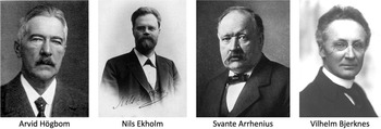
Figure 2.1 Members of the Stockholm Cosmic Physics Society: Arvid Högbom (Geologist, mapped fluxes of CO₂ in the atmosphere); Nils Ekholm (Meteorologist, studied causes of the ice ages); Svante Arrhenius (Chemist, developed first model of climate change); Vilhelm Bjerknes (Physicist, worked out the equations for weather prediction).

This group of scientists was remarkably diverse. Geologists from the Swedish Geological Survey came to discuss the geological eras of the past. Weather forecasters from the Meteorological Office came to discuss the forces that shape weather patterns. Biologists from the Museum of Natural History came to discuss fossil records and evolution. Astronomers came to discuss comparisons between the Earth and other planets and moons.

In the group were two remarkable young scientists, Svante Arrhenius and Vilhelm Bjerknes. Both served as lecturers in the early 1890s at the Stockholm Högskola (which later became the University of Stockholm) and both were promoted to professors of physics in the same year: 1895. Bjerknes was a mathematical physicist, with interests in magnetic fields and fluids – we’ll come back to his work in more detail in Chapter 3. Arrhenius was a chemist who went on to win a Nobel Prize for his research on acids. Both were inspired to apply their work to weather and climate by the discussions at the meetings of the Society.

Arrhenius was particularly intrigued by a series of talks by the geologist Arvid Högbom about carbon, the basic building block for all life on Earth. Högbom had mapped out what was, at the time, the most complete account of the carbon cycle, and had taken detailed measurements of the amount of gaseous “carbonic acid” in the atmosphere.¹ Today we call it carbon dioxide (or CO₂ for short). Högbom had studied where carbon dioxide comes from and where it goes. He had identified six different sources: erupting volcanoes; meteorites burning up in the upper atmosphere; vegetation as it decomposes or burns (in which he included the burning of coal and oil); release of carbon trapped in rocks by chemical reactions; rock fracturing; and seawater as it warms under the sun. He had identified three ways carbon dioxide is removed: rock weathering (in which carbon dioxide dissolves in rainwater and reacts with limestone to produce calcium bicarbonate); absorption by plants; and absorption by the oceans.

Högbom thought these sources and sinks would balance each other, so the amount in the atmosphere wouldn’t change much over time. But he couldn’t be sure, because there was no easy way to measure some sources, such as meteorites. This suggested a rather radical idea: perhaps the amount of carbon dioxide in the atmosphere did change over time. When the society members pressed him on the question, Högbom thought only one of his sources would be big enough to radically change things: volcanoes. He never imagined that human use of fossil fuels would eventually far outstrip anything volcanoes produce, because, in the nineteenth century, the human contribution to CO₂ in the atmosphere was too small to measure.

Early in 1893, the society turned its attention to one of the biggest scientific mysteries of the time: what had caused the ice ages? Nils Ekholm, from the Swedish Meteorological Office, had just returned from an expedition to Spitsbergen, a large island halfway between Norway and the North Pole. He came to the society to give a talk on the latest findings about the ice ages, when the world was on average 5°C to 6°C cooler, and Northern Europe was covered in ice sheets. The topic was particularly salient for Scandinavian scientists: evidence of the retreat of the glaciers was all around them. Ekholm’s talk was followed by a lively discussion of the latest hypotheses about possible causes of the ice ages. Some members thought that changes in the height of the land were to blame, but others pointed out this wouldn’t explain why ice ages seemed to come and go on a regular basis, nor why the temperature changes affected the whole planet.

It was Svante Arrhenius who connected the dots between Högbom’s work on the carbon cycle and Ekholm’s question about the ice ages. It was well known at the time that gases such as carbon dioxide help keep the planet warm. What if there was less CO₂ during the ice ages? Wouldn’t that explain everything? The idea was largely dismissed by the society, as none of them believed the carbon in the atmosphere could change enough to affect the temperature of the planet. But Arrhenius was undeterred. Inspired by Högbom’s observations of how carbon dioxide enters and leaves the atmosphere, he built a climate model to show that his idea was plausible.

Climate Science in the Nineteenth Century

Arrhenius was an unusual scientist, at least by today’s standards.² His curiosity took him from an early career in chemistry, through physics and cosmology, to a study of toxins. As a student, he was always interested in big conceptual questions, which sometimes led him to neglect his laboratory work, much to the dismay of his professors. When he received his PhD, his professors didn’t think much of his work, and gave him the lowest possible passing grade. He, in turn, thought his professors were stuffy traditionalists, resistant to the latest ideas in the field. He spent the next few years as a research fellow at several labs in Germany and Holland, where he developed the theories of ionization of acids in water that would later earn him a Nobel Prize. He returned to Sweden in 1891 for a teaching job at the Stockholm Högskola. His German friends thought this was a bad move – all the interesting work was being done in Western Europe. But it was at the Högskola that Arrhenius found the rich intellectual environment he craved. He shifted his interests from chemistry to physics, driven, no doubt, by the broad set of topics discussed at the Cosmic Physics Society, of which he was a founding member.

We tend to think of science as advancing mainly through the work of lone geniuses, but this is largely because it’s easier to tell the story if we can give credit to just one person. Arrhenius himself was clearly a brilliant scientist. But, as is usually the case, his achievement was only possible because it built on the work of many others. The basic theory behind his model wasn’t new. Nor was the data he used for the calculations. But his obsessive pursuit of an answer to a very specific question drove him to tie together the work of physicists, astronomers, and meteorologists in a remarkable new way. In his 1896 paper, Arrhenius phrased the question as: “Is the mean temperature of the ground in any way influenced by the presence of heat-absorbing gases in the atmosphere?” The answer he sought was a precise quantification of how much ground temperatures would change if the amount of CO₂ in the atmosphere changed.

The idea that the temperature of the planet could be analyzed as a mathematical problem dates all the way back to the work of the French mathematician, Joseph Fourier,³ in the 1820s. Fourier had studied the up-and-down cycles of temperature between day and night, and between summer and winter, and had measured how deep into the ground these heating and cooling cycles reach. It turns out they don’t go very deep. At about 30 metres below the surface, temperatures remain constant all year round, showing no sign of daily or annual change. Today, Fourier is perhaps best remembered for his work on the mathematics of such cycles, and the Fourier transform, a technique for discovering cyclic waveforms in complex data series, was named in his honour.

For a planet as a whole, Fourier reasoned as follows. The temperature of any object is due to the balance of heat entering and leaving it. If more heat is entering, the object warms up, and if more heat is leaving, it cools down. For planet Earth, Fourier pointed out there are only three possible sources of heat: the sun, the Earth’s core, and background heat from space. His measurements showed that the heat at the Earth’s core no longer warms the surface, because the diffusion of heat through layers of rock is too slow to make a noticeable difference. He thought that the temperature of space itself was probably about the same as the coldest temperatures on Earth, as that would explain the temperature reached at the poles in the long polar winters. On this point, he was wrong – we now know space is close to absolute zero,⁴ a couple of hundred degrees colder than anywhere on Earth. But he was correct about the sun being the main source of heat at the Earth’s surface.

Fourier also realized there must be more to the story than that, otherwise the heat from the sun would escape to space just as fast as it arrived, causing night-time temperatures to drop back down to the temperature of space – and yet they don’t. We now know this does happen on the moon, where temperatures drop by hundreds of degrees after the lunar sunset. So why not on Earth?

The Greenhouse Effect

The solution lay in the behaviour of “dark heat,” an idea that was new and mysterious to the scientists of the early nineteenth century. Today we call it infra-red radiation. Both Fourier and Arrhenius referred to it as “radiant heat” or “dark rays” to distinguish it from “light heat,” or visible light. But really, they’re just different parts of the electromagnetic spectrum (see Figure 2.2). Any object that’s warmer than its surroundings continually radiates some of its heat to those surroundings. If the object is hot enough, say an oven, you can feel this “dark heat” if you put your hand near it, although we can only feel infra-red rays when the oven is pretty hot.⁵ But even objects that we think of as pretty cold still radiate a small amount of infra-red to their surroundings. When you heat up an object, it radiates more energy, and the kind of energy it radiates spreads up the spectrum from infra-red to visible light – it starts to glow red, and then, eventually white hot.

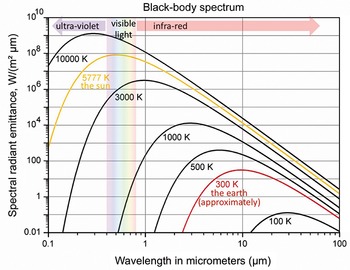
Figure 2.2 At different temperatures, objects radiate energy in different parts of the spectrum. A hotter object radiates more heat at shorter wavelengths on the electromagnetic spectrum than a cooler object. The sun radiates across the ultra-violet, visible, and infra-red, with the peak of its emissions in the visible spectrum. The Earth, being much cooler, emits only in the infra-red part of the spectrum. The shorter the wavelength, the more energy the rays carry, which is why very short wavelength ultraviolet light is dangerous to human health.

(CC-BY-SA Wikimedia Commons user: Sch)

Fourier’s theory was elegantly simple. Because the sun is so hot, much of its energy arrives in the form of visible light, which passes through the atmosphere relatively easily,⁶ and warms the Earth’s surface. As the Earth’s surface is warm, it also radiates energy. But the Earth is a lot cooler than the sun, so the energy the Earth radiates is in the form of dark heat (see Figure 2.3). Dark heat doesn’t pass though the atmosphere anywhere near as easily as light heat, so this slows the loss of energy back to space.

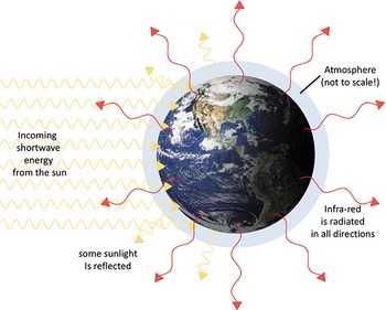
Figure 2.3 The surface temperature of the Earth is determined by the balance between the incoming heat from the sun (shortwave rays, mainly visible light and ultra-violet) and the outgoing infra-red, radiated in all directions from the Earth. The incoming short-wave rays passes through the atmosphere much more easily than the long-wave outgoing rays.

To explain the idea, Fourier used an analogy with a hotbox, a very well-insulated wooden box, painted black inside, with three layers of glass in the lid, used by explorers as a solar oven. The sun would heat the inside of the box to over 100°C, even on high mountains, where the outside air is much colder. The glass lets the sun’s rays through, but slows the rate at which the heat can escape. Fourier argued that layers of air in the atmosphere play a similar role to the panes of glass in the hotbox, by trapping the outgoing heat; like the air in the hotbox, the planet would stay warmer than its surroundings. A century later, Fourier’s theory came to be called the “greenhouse effect,” perhaps because a greenhouse is more familiar to most people than a hotbox.⁷

Experimental Evidence

While Fourier had observed that air does indeed trap some of the heat from the ground, it wasn’t clear why until the 1850s, when scientists began to experiment with the heat trapping effects of different gases (see Figure 2.5). The first of these was Eunice Foote, an American scientist who set up a series of experiments to discover why air in a valley is warmer than air up a mountain. Foote’s experiments showed that denser air absorbs more of the sun’s heat. She then went on to show that air with more moisture and air with more carbonic acid also absorb more heat, and retain it longer. These remarkable experiments, reported in Scientific American⁸ in September 1856, led her to hypothesize that if, for planet Earth, “at one period of its history the air had mixed with it a larger proportion [of CO₂] than at present, an increased temperature … must have necessarily resulted.”⁹ Unfortunately, her experiments appear to have been largely forgotten, until her work was rediscovered in 2011, but she is now credited as the first scientist to discover carbon dioxide is responsible for global changes in climate.

In Foote’s experiment, she pumped the gases into glass cylinders, heated directly by the sun. But glass is largely opaque to infra-red – dark heat – so her experiment missed an important piece of the puzzle. A few years later, the English scientist John Tyndall devised a more elaborate experiment¹⁰ to find out if different gases would absorb dark heat. Tyndall’s experiments put different gases into a four foot brass tube, sealed at both ends with disks of salt crystal, because, unlike glass, salt is transparent to dark heat. Two pots of boiling water provided sources of heat, and a galvanometer compared the heat received directly from one heat source (A) with heat from the other (B) after it had passed through the tube of gas. Figure 2.4 shows a drawing of his apparatus.

Figure 2.4 Tyndall’s experimental equipment for testing the absorption properties of different gases. The brass tube was first evacuated, and the equipment calibrated by moving the screens until the temperature readings from the two heat sources were equal. Then the gas to be tested was pumped into the brass tube, and change in deflection of the galvanometer noted.

(Adapted from Tyndall (Reference Tyndall1861))

Figure 2.5 Nineteenth-century scientists who contributed to the discovery of the greenhouse effect.

When Tyndall filled the tube with dry air, or oxygen, or nitrogen, there was very little change. But when he filled it with the hydrocarbon gas ethene, the temperature at the end of the tube dropped dramatically. This was so surprising that he first suspected something had gone wrong with the equipment – perhaps the gas had reacted with the salt, making the ends opaque? After re-testing every aspect of the equipment, he finally concluded that it was the ethene gas itself that was blocking the heat. He went on to test dozens of other gases and vapours, and found that more complex chemicals such as vapours of alcohols and oils were the strongest heat absorbers, while pure elements such as oxygen and nitrogen had the least effect.

Why do some gases allow visible light through, but block infra-red? It turns out that the molecules of each gas react to different wavelengths of light, depending on the molecule’s shape. A good analogy is the way sound waves of just the right wavelength can cause a wine glass to resonate. Each type of molecule will vibrate when certain wavelengths of light hit it, making it stretch, contract, or rotate. So the molecule gains a little energy, and the light rays lose some. Scientists use this effect to determine which gases are in distant stars, because each gas makes a distinct pattern of dark lines across the spectrum from white light that has passed through it, marking the wavelengths at which that gas absorbs energy.

Tyndall noticed that gases made of more than one element, such as water vapour (H₂O) or carbon dioxide (CO₂), tend to absorb more energy from the infra-red rays than gases made of a single type of element, such as hydrogen (H₂) or oxygen (O₂). He argued this provides evidence of atomic bonding: it wouldn’t happen if water was just a mixture of individual oxygen and hydrogen atoms. He was clearly on the right track here. We now know that what matters isn’t just the existence of molecular bonds, but whether the molecules are asymmetric¹¹ – after all, oxygen gas molecules (O₂) are also pairs of atoms bonded together. The more complex the molecular structure, the more asymmetries it has, and the more modes of vibration and spin the bonds have, allowing them to absorb energy at more wavelengths. Today, we call any gas that absorbs parts of the infra-red spectrum a greenhouse gas. More complex compounds, such as methane (CH₄) and ethene (C₂H₄), absorb energy at even more wavelengths than carbon dioxide, making them stronger greenhouse gases.¹²

Tyndall’s experiments showed that greenhouse gases absorb infra-red even when the gases are only present in very small amounts. Tyndall concluded that, because of its abundance in the atmosphere, water vapour is responsible for most of the heat trapping effect that keeps the Earth warm, with carbon dioxide second.¹³ Some of the other vapours he tested have a much stronger absorption effect, but are so rare in the atmosphere they contribute little to the overall effect. Like Foote, Tyndall clearly understood the implications of these experiments for the Earth’s climate, arguing that it explains why, for example, temperatures in dry regions such as deserts drop overnight far more than in more humid regions.¹⁴ In the 1861 paper describing his experimental results, Tyndall argued that any change in the levels of water vapour and carbon dioxide, “must produce a change of climate.” He speculated that “such changes in fact may have produced all the mutations of climate which the researches of geologists reveal.”¹⁵

A Model Needs Data

Although the greenhouse effect was known by the time Arrhenius developed his model, what was missing was a way to calculate the size of the effect. Some scientists had already attempted this. For example, in 1837, the French physicist Claude Pouillet invented an instrument known as a pyrheliometer to measure the heat energy we receive from the sun, and obtained the remarkably accurate measurement of 1.76 calories per minute per square cm. He later attempted to calculate how much of the Earth’s outgoing infra-red energy is absorbed by the atmosphere, but, as Arrhenius discovered, Pouillet got these calculations wrong.¹⁶

So in one sense, Arrhenius was merely replicating the work of earlier scientists, checking they were correct, and finding errors. But he went well beyond what anyone else had attempted in his quest to explain the cause of the ice ages.

For precise calculations, Arrhenius needed data. Tyndall’s experimental data didn’t help, because measurements of the absorption effect in a four-foot tube don’t really tell you how the effect works when infra-red rays pass through the full height of the atmosphere. Arrhenius needed data on how much of the existing greenhouse effect could be attributed to each of water vapour and carbon dioxide, the two main greenhouse gases – he called them “selective absorbers” – when they are mixed in the exact proportions that occur in the atmosphere. And he needed data on what happens if you vary the amount of each gas.

Today, we measure the outgoing infra-red at the top of the atmosphere directly, using satellites (see Figure 2.6), and we have excellent data showing how absorption levels have changed over time, from the beginning of the satellite era in the 1970s to the present day. Analyzing the contribution of water vapour and CO₂ is now relatively straightforward, because we can compare the heat emitted in wetter and drier regions, and we can compare changes over the last few decades, as carbon dioxide levels have risen. These satellite readings demonstrate not only that Fourier’s theory is correct, but also (spoiler alert) increasing levels of carbon dioxide have indeed reduced the rate at which the planet loses heat to space.¹⁷

Figure 2.6 The fingerprint of greenhouse gases, as detected by the Nimbus 4 satellite on July 31, 1970, with theoretical radiation curves (dashed lines) shown for comparison. With no greenhouse gases, the satellite would see infra-red rays from the ground, matching the upper dashed line for expected radiation at 280 K (about 7°C), the local ground temperature when these measurements were made. The dips in the solid line show parts of the spectrum where each greenhouse gas blocks the infra-red from the ground. In these parts of the spectrum, the satellite only sees rays from higher in the atmosphere, where the air is cooler (lower dashed line).

(Gavin Schmidt/NASA GISS)

But Arrhenius was working long before we had satellites – even before the Wright brothers had demonstrated a working airplane. Luckily, he had access to observational data collected by an American, Samuel Pierpont Langley, one of the Wright brothers’ fiercest competitors. A remarkable inventor, Langley might have beaten the Wright brothers to the first working airplane if he hadn’t chosen to use a catapult for the take-off. Langley had also invented an instrument for making very precise measurements of infra-red energy. His “bolometer” was widely admired; it was accurate enough to measure the heat from a cow at a quarter of a mile away.

As director at the Allegheny Observatory in Pittsburgh, Langley put his bolometer to good use measuring the temperature of the moon. When we see the moon shining in the night sky, what we actually see is sunlight reflected from the moon’s surface. But as the sun heats the surface of the moon, the moon also radiates its own “dark rays” – infra-red energy. As we saw in Figure 2.2, objects at different temperatures emit energy across different parts of the spectrum. If Langley could measure the amount of energy the moon gave off at each wavelength, he could calculate its temperature. He used a prism made from a pure crystal of salt to separate the wavelengths of infra-red coming from the moon, in the same way that a glass prism can separate sunlight into the colours of the rainbow. Readings from the bolometer could then be used to calculate the energy received at each of 21 different wavelengths across the infra-red spectrum.¹⁸

Between 1883 and 1888, Langley and his colleague, Frank Very, used the bolometer to take detailed measurements of the infra-red spectrum from the moon, at different times of day and night. In 1890 they published the first detailed estimate of its surface temperature. The full moon was, they found, around 100°C – the temperature of boiling water. During a full moon, the whole of the side of the moon that is visible from Earth is bathed in sunlight, so this is actually the hottest the moon gets. Modern measurements show the moon’s surface temperature varies dramatically, as hot as 120°C, during the lunar day, but dropping as low as −150°C on the dark side of the moon,¹⁹ much colder than anywhere on Earth. The Apollo astronauts’ spacesuits had to protect them from both extreme heat and extreme cold.

These measurements solved one of Arrhenius’s biggest challenges. He needed data on how much heat from the Earth’s surface is absorbed as it passes up through the atmosphere. Langley and Very’s measurements were almost as good: the infra-red rays from the moon had passed down through the Earth’s atmosphere, and so would be absorbed by about the same amount. Not only that, but they had measured the rays from the moon when it was at different heights in the sky. This meant the rays had passed through different amounts of atmosphere for each reading. The more atmosphere they passed through, the more greenhouse gases they encountered (see Figure 2.7). Furthermore, Langley and Very had carefully recorded the humidity for each reading; in drier air there was less water vapour to absorb the infra-red. This gave Arrhenius the range of absorption data he needed. By comparing the measurements for each wavelength of infra-red in drier and wetter air, and in different thicknesses of atmosphere, Arrhenius could calculate “absorption coefficients” for varying amounts of H₂O and CO₂.

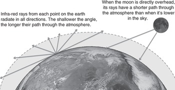
Figure 2.7 The length of the path of an infra-red ray as it passes through the atmosphere depends on its angle. On longer paths, the ray passes through more greenhouse gases. Most of the paths taken by outgoing infra-red from the surface of the Earth are longer than the vertical height of the atmosphere. Arrhenius calculated the average length of these paths to be about 1.6 times the vertical height of the atmosphere. Similarly, the moon’s rays pass through different amounts of atmosphere as the moon crosses the sky. (Diagram not to scale!)

As with any observational data, there are many potential sources of error in the readings, from human mistakes in recording the measurements, to problems with the instrument and the way it is used. Arrhenius picked the readings that appeared to be most consistent with one another, and used the changes in humidity and angle of elevation to deduce the absorption fraction for each of the two gases at each of Langley’s 21 measured wavelengths of infra-red. Today we call this a line-by-line analysis, and it has become a standard technique in satellite data analysis. The result is an absorption “fingerprint” for each gas across the infra-red spectrum. Arrhenius tested his results by checking them against the rest of Langley and Very’s data,²⁰ which again is now a standard technique in data analysis: use some of the data to compute a relationship, and the remainder of the data to test it.

With this data, most of the puzzle pieces were in place (see Figure 2.8). Fourier provided the theory, from basic physics, that the sun warms the Earth during the day, and the atmosphere slows the loss of this heat, keeping the planet warm. Tyndall provided the experiments that demonstrated why: some gases, such as water vapour and carbon dioxide, “selectively absorb” parts of the infra-red spectrum. And finally, Langley and Very had detailed observations of how much infra-red is absorbed along different paths through the atmosphere, at various levels of humidity. By putting these pieces together in the right way, Arrhenius could build a computational model of the Earth’s energy balance.

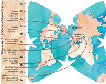
Figure 2.8 Timeline of key milestones in nineteenth-century understanding of the greenhouse effect.

(Watercolour map by Stamen Design)

Putting the Model Together

In essence, a model is just a set of equations that capture the relationships described in a scientific theory. Running a model means putting some observational data into these equations, to calculate other values that cannot be observed directly.

The starting point for Arrhenius’s model was an equation that captures the key idea in Fourier’s theory: for the average temperature of the planet to be stable over the years, the incoming energy from the sun must equal the outgoing energy lost at the top of the atmosphere. Temperatures do rise and fall across the planet, because different regions receive more or less sunlight at different times of the year, and the winds and ocean currents move the heat around. But overall, these exchanges of heat balance out, so that, at least during the nineteenth century, no part of the planet was experiencing a year-on-year warming or cooling trend. The planet was in radiative balance.

The equation needed to express this was first worked out in 1879 by the Austrian physicist Jožef Stefan, who discovered the relationship between the temperature of an object and the energy it radiates.²¹ Stefan found that the rate at which an object radiates heat is proportional to its temperature (in Kelvin) raised to the power of four.²² The fact that there’s a power of four in the equation means the rate at which energy is radiated grows very rapidly with small increases in temperature. For example, if you put a pan on the stove and turn on the heat, the temperature of the pan rises, but as it does, the amount of heat it radiates rises even faster. The pan heats up only until it is losing energy as fast as it is receiving it from the stove: it finds a new equilibrium.

Stefan’s equation describes an “ideal” object, one that absorbs perfectly all the radiative heat it receives, and radiates heat out again with no impediment. Such an object reflects no light, so would appear completely black – in thermodynamics, it’s called a blackbody. But most objects don’t absorb and emit radiative heat perfectly – an object with a paler surface will reflect some heat, rather than absorbing it. Shiny surfaces do this well: they reflect incoming heat and light away from the object (which is why they look shiny), and, perhaps less obviously, they reflect internal heat back towards the inside, which means they cool down more slowly. So shiny materials make good coat linings and emergency survival blankets. Stefan’s student, Ludwig Boltzmann, found the original equation still works for such objects (known as “grey bodies”) if you adjust²³ for the fraction of incoming rays that are reflected rather than absorbed. For a planet, the percentage of sunlight reflected back to space is called the albedo. The Earth currently reflects around 30% to 35% of the incoming sunlight, due to all the white snow and clouds. For other things, including gases, it’s more usual to talk about what fraction of heat they absorb, which is the inverse of albedo – it’s the fraction of rays (at each wavelength) that will pass into them. Arrhenius called this their absorption coefficient. Today we call it emissivity – because any insulating effect that hampers how an object absorbs heat also hampers the heat being emitted again.

With the surface and the atmosphere acting as grey bodies, it’s possible to write equations for the flows of energy between them. The key insight is the energy balance at the top of the atmosphere – as shown in the schematic of the model in Figure 2.9. If the climate doesn’t change from one year to the next, then the total input of energy from the sun – over the course of a year – must be the same as the total output of energy lost to space. Inputs and outputs must balance.²⁴ The Stefan–Boltzmann equation then allows you to work out what temperature the ground and atmosphere must to be to make all these energy flows balance.

Figure 2.9 Schematic of Arrhenius’s model, for a patch of the Earth’s surface and the column of air above it. All energy flows are in “watts per square meter” of ground surface. The diagram shows heat received from neighbouring columns in green, incoming (shortwave) sunlight in yellow, infra-red emitted by the ground in red, and infra-red emitted by atmosphere in blue. The three equations express that in-flows and out-flows in each part of the system must balance. The detailed equations appear in Arrhenius (Reference Arrhenius1896).

The model has the sun as the main source of heat. Some of the sun’s heat warms the air, and some warms the Earth’s surface. Of the sunlight that reaches the surface, some is absorbed, and some reflected directly back out to space. The latter depends on the Earth’s albedo, which varies across the planet. Arrhenius spent considerable effort coming up with estimates for the albedo of different types of surface: fresh snow, old snow (which is darker because it gets dirty), ocean, vegetation, and soils. His estimates were remarkably close to modern measurements. Because some parts of the surface are obscured by clouds, which reflect sunlight directly back into space, Arrhenius estimated the “average cloudiness” of the sky, and adjusted his albedo values to account for this too.

The complication is that different locations on the planet receive different amounts of sunlight. Surface temperature, albedo, and humidity all vary by location too. So the energy balance will be different at each location. To address this, Arrhenius divided up the surface of the planet into a regular grid, with grid cells each spanning 10° of latitude and 20° of longitude (see Figure 2.10) – but omitting the polar regions, where very little data had been collected. He could then apply the energy balance equation to each grid cell.

Figure 2.10 The grid used in Arrhenius’s model. The grid has 13 bands of latitude from 60° South to 70° North, each divided into 18 cells around the planet (covering 20° of longitude each). This grid covers nearly all the major landmasses except Antarctica and Northern Greenland, as reliable weather data for the polar regions wasn’t available in the nineteenth century. This 13 × 18 grid has 234 cells.

This choice of grid was convenient because it was also used in published weather maps²⁵ compiled by the Scottish meteorologist Alexander Buchan, who had calculated the average temperature for each grid cell, for each month of the year. Arrhenius converted these to seasonal averages, to reduce the amount of data he had to deal with, but without losing the ability to study whether seasonal changes mattered. This gave him four seasonal temperature values for each of the 234 grid squares – a total of 936 data points. He then did the same for humidity data.²⁶

Like modern climate models, Arrhenius’s model is built from the laws of physics. However, it’s much simpler than modern models: it treats the vertical column of air in each grid cell as though it were a single unit, with a single average temperature. In reality the higher you go, the colder the air gets. To check how much this simplification mattered, Arrhenius tested a calculation for a two-layer version of his model, with a lower warmer layer of air that exchanges heat with the surface, and a higher, cooler layer that loses heat to space. He concluded the results were similar enough that he could just work with a one-layer version to cut down the number of calculations. Nowadays, we have supercomputers to do the work, so modern climate models use much smaller grid cells, and divide the air into dozens of different layers to calculate the exchange of heat between each layer and those above and below it.

Despite all the data Arrhenius had collected from existing weather maps, there were still many unknowns. These include, for each grid cell, heat received from the sun, the fraction absorbed directly by the air, and horizontal heat exchanges with neighbouring grid cells. To simplify things, Arrhenius assumed none of these values would change when you vary the amount of greenhouse gases, so he could treat them as constants in each grid cell, for each season. Today, we would call these model parameters – values that cannot be calculated, so must be estimated from observational data. Obtaining accurate measurement for parameters like these is still tricky in today’s models. For Arrhenius it was impossible. Instead, he re-arranged the equations to collect all of these unknown values together as a single (unknown) parameter, which he called K.

This new form of the equation could calculate surface temperature for any location on the planet, as long as you had the local values for surface albedo, the atmospheric emissivity, and the parameter K.²⁷ In Arrhenius’s experiments, emissivity would be the main input to the model. To test the effect of different concentrations of the two main greenhouse gases, you would select the relevant values from his tables of absorption coefficients to provide this input.

The unknown constant parameter K in Arrhenius’s equation is different for each location, and each season, because it depends on the amount of sunlight received (which is larger closer to the equator, and closer to summer), and the amount of heat exchanged horizontally (which depends on prevailing winds and ocean currents). However, Arrhenius realized he could calibrate the model to find each value for K by running his model “backwards” – given he knew the average surface temperature for each location at each time of year. He could then run the model “forwards” to calculate how the temperature would change with different levels of CO₂.

Using the Model

The key equation in Arrhenius’s model calculates how the surface temperature (at a particular location and a particular time of year) will change if the levels of water vapour and carbon dioxide in the atmosphere change. Because his original question was about the cause of the ice ages, Arrhenius was mainly interested in what happens if there is less of these greenhouse gases. But the model works just as well for increases.

Of the two gases, water vapour is by far the more abundant in the atmosphere. On average, about 4% of the atmosphere is water, while carbon dioxide is around 0.04%.²⁸ So there are roughly a hundred times more H₂O molecules in the atmosphere than there are CO₂ molecules. So why did Arrhenius focus on carbon dioxide rather than water vapour? Why, for that matter, do modern climate scientists also focus on carbon dioxide?

The answer is that natural cycles of evaporation and precipitation tend to stabilize the amount of water vapour in the atmosphere, so that the average amount only varies when the air temperature changes – hotter air can hold more moisture. In contrast, the amount of carbon dioxide in the atmosphere can vary almost without limit. So the atmosphere can retain large changes in the amount of CO₂ over long time periods, but not large swings in the amount of water.

In fact, any given molecule of CO₂ might only stay in the atmosphere for a few years, as CO₂ is regularly absorbed by plants and soils, and some of it dissolves in the surface waters of the ocean.²⁹ But plants and soils also emit CO₂ as they decompose over the winter. And the ocean re-emits CO₂, especially when it warms up. So, over a period of a few years, any additional CO₂ gets shared out, with plants, soils, oceans, and atmosphere each taking a share. The atmosphere’s share is, roughly speaking, about half of any new CO₂ produced, for example from burning coal and oil. Högbom’s other carbon sinks all operate much more slowly – on a geological timescale – taking thousands of years to absorb CO₂ from the atmosphere.

Thinking this through led to one of Arrhenius’s most important insights: changes in water vapour don’t cause climate change, but are a result of it. In other words, water vapour forms a feedback loop. If something else warms the atmosphere, the air will hold more water vapour, which will then produce more warming. Similarly, if something else causes cooling, the resulting loss of water vapour will accelerate that cooling. This water vapour feedback loop would amplify any change in global temperature. This insight was both exciting and frustrating. Exciting, because it helped his hypothesis about carbon dioxide causing the ice ages – a smaller change in carbon dioxide would be amplified by the water vapour feedback to cause a bigger change in temperature. But frustrating, because it would complicate the model.

Arrhenius handled this feedback loop by applying the model in two steps. First he “ran” the model once, to calculate the temperature change from a decrease (or increase) in carbon dioxide, with no change in water vapour. Then, for each output, he calculated how this temperature change would affect water vapour, assuming no change in relative humidity – the fraction of moisture the air actually holds, compared to how much it could hold. This assumption isn’t perfect, but is close enough to give reasonable results. Then he “ran” the model again to calculate how much more the temperature would change in response to this increased water vapour.

To do this for his entire grid would require 936 calculations at each step: 2,808 calculations in all – and when repeated for each season that would mean 11,232 calculations! All of these would have to be done by hand, so Arrhenius saved himself a lot of effort by first calculating an average seasonal temperature for each latitude band, leaving him with 624 calculations for each “run” of the model. Today, we would call this a one-dimensional model, where the dimension is latitude – a full three-dimensional model would include longitude and height in the atmosphere too.

Water vapour feedback is not the only feedback loop in the global climate system, and understanding these feedbacks is important for developing good models. Arrhenius was aware of some of them, but could not include them without making the calculations unmanageable. Instead, he dealt with them by reasoning about how they might affect the model results. For example, snow and ice create a feedback loop, because they alter the surface albedo. A little warming would melt some of the ice and snow, replacing it with darker ocean or soil, which absorbs more heat. This amplifies the warming. Similarly, a little cooling allows ice and snow areas to expand, raising the albedo to reflect more heat directly back to space, and hence amplifying the cooling. This ice-albedo feedback is strongest at the edges of existing ice fields, so Arrhenius reasoned the temperature changes would be bigger in the polar regions if he had included this effect.

Today’s models incorporate more of these feedback effects, but modellers still have to make similar trade-offs between computability and completeness. Expert judgment is needed to identify feedbacks that might matter, and to decide whether they can be included in the model. This also illustrates another feature of both Arrhenius’s work and today’s models: the output of a computer model has to be interpreted very carefully, based on an understanding of what the model includes and what it leaves out.

The Results

Arrhenius laid out his results in a table (shown in Figure 2.11), giving the computed temperature change for each latitude, for each season of the year, under various scenarios for decreased or increased carbon dioxide. The rows correspond to the 10° latitude bands. The five main columns show scenarios for five different levels of CO₂: reduced by one third (0.67), and increased to 1.5, 2, 2.5, and 3 times the current level. Within each major column is a sub-column for each season, followed by an annual average. The numbers represent changes in surface temperature, in degrees centigrade.

Figure 2.11 Raw results from Arrhenius’s model, showing expected temperature change in degrees centigrade, for each latitude (the rows), and each season, for a range of scenarios from reducing CO₂ (“carbonic acid”) by a third, up to increasing it by a factor of three.

(Reproduced from Arrhenius (Reference Arrhenius1896))

Despite the many simplifications, developing and using the model was hard work. The data he had gathered for his grid consisted of more than 3,000 data points, and the five scenarios shown in Figure 2.11 required 3,120 separate calculations. The work took Arrhenius over a year, from December 1894 to January 1896. In his letters at the time he commented on how tedious the work was, but also expressed his determination to complete it, so he could answer his original question about the ice ages.

The table suggests that changing levels of carbon dioxide could indeed cause the kinds of temperature swing Arrhenius had hypothesized. He also realized the relationship between CO₂ levels and temperature isn’t linear – you get about the same rise (or fall) in temperature for each doubling (or halving) of carbon dioxide, which is why today we use doubling of CO₂ – the Charney sensitivity – as a benchmark for comparing models.

Arrhenius’s model also predicts that the effect would be different in different parts of the world. The temperature changes are larger over land than over the ocean, and larger in the northern hemisphere than the southern – because the southern hemisphere has a lot more ocean. The model predicts larger temperature changes wherever and whenever it is currently coolest: towards the poles, and during the winters. Arrhenius also predicted larger changes for nighttime temperatures than daytime, although this isn’t shown in the table – Arrhenius did a separate “run” of the model for day versus night.

These effects all arise directly from the basic physics represented in the model. Greenhouse gases work by trapping outgoing heat. Therefore they have the biggest impact when there is more heat leaving the Earth’s surface than arriving: after the heat of the day; after the summer has ended; and on the parts of the planet that receive less sunlight anyway. Arrhenius summarized his results: “If carbonic acid content rises, temperature differences between land and sea, between summer and winter, between night and day, and between equator and temperate zones will be levelled out, at least for habitable parts of the Earth’s surface. The reverse will be true if the carbonic acid content diminishes.”³⁰ This is quite a remarkable set of predictions, as none of these effects had been worked out before Arrhenius built his model. And every one of them turned out to be correct.

But what of the question that drove him to develop the model in the first place: could carbon dioxide be responsible for the ice ages? The results suggest that CO₂ would need to drop to nearly half its late nineteenth-century level to produce the global cooling of about 5°C that occurred during the last ice age.³¹ Arrhenius took this as a very encouraging result, as there is no physical reason why it couldn’t have happened, given Högbom’s analysis of carbon flows into and out of the atmosphere. However, the model only says what would have happened if carbon dioxide levels fell this much; it doesn’t help answer why they would fall in the first place.

What about the scenarios for increased CO₂? It seems odd that he would have included results for doubled and trebled CO₂, given his primary interest was in explaining the ice ages. But Högbom had pointed out the amount of carbon in the atmosphere is insignificantly tiny compared to the vast stocks tied up in limestone rocks. The idea that geological processes might, over time, release these to the atmosphere was certainly worth exploring.

And Arrhenius lived during the age of steam. There were no cars and no planes; the dominant modes of transport, other than the horse, were steam trains and steam ships. Coal was the magic fuel that powered the industrial revolution, and the effects of coal smoke in cities across Europe was easy to see: smog swirled around the cities, and bigger cities such as London were known for their intense fogs, known as “pea-soupers,” in the second half of the nineteenth century. Högbom had included burning of coal as a source of atmospheric carbon dioxide, so it made sense for Arrhenius to explore where this might lead. He took Högbom’s measures of carbon emissions from coal burning, and projected them into the future. At the time, the best estimate was that each year about 0.7 gigatonnes of carbon were being released globally from coal use – about 1/900th of the total amount already in the atmosphere. As a chemist, Arrhenius also knew that increased levels of CO₂ in the atmosphere would increase the rate at which it dissolves in seawater. He calculated that about five sixths of these emissions from coal would eventually be absorbed by the oceans. That left an annual increase of CO₂ in the atmosphere that would, at the time, be too small to measure.³²

Using these numbers, he calculated it would take 54 years to increase atmospheric CO₂ by 1%, and about 3,000 years to increase CO₂ levels by 50%, for which his model indicated global temperatures would rise by about 3.4°C. His reaction to this might resonate today with anyone who lives in a cold climate: “we would have some right to indulge in the pleasant belief that our descendants, albeit after many generations, might live under a milder sky and in less barren natural surroundings than is our lot at present.”³³ He had no way to foresee the imminent and dramatic rise in the use of fossil fuels.

A Sceptical Audience

Unfortunately, Arrhenius’s work was largely ignored by other scientists at the time. His closest colleagues were full of admiration: Högbom and Ekholm, whose work had inspired Arrhenius to set off on this path in the first place, were delighted with his model. But others in the Stockholm Society were not so impressed. Nobody attempted to replicate his calculations, as the effort would have been too great, and the results didn’t seem plausible enough to warrant it. While the idea that water vapour and carbon dioxide play an important role in keeping the Earth warm was widely accepted, the notion that changes in these gases might explain the ice ages was dismissed as ridiculous. Besides, another theory about the ice ages was rapidly gaining ground: regular changes in the Earth’s orbit appeared to be the best explanation.

Perhaps the biggest reason that few people took the work seriously was a devastating critique by another Swedish scientist, Knut Ångström. Ångström’s father, Anders, was renowned for his work developing the science of spectroscopy. Knut was following in his father’s footsteps. He had held a lectureship in physics at the Stockholm Högskola before Arrhenius, and was now a professor at the University of Uppsala, 70 km north of Stockholm, where he was working on making precise measurements of the sun’s energy. By comparison, Arrhenius was the newcomer, seen to meddle in fields in which he hadn’t been trained.

Ångström argued there were two key problems with Arrhenius’s model. First, Langley’s data wasn’t reliable enough, and indeed, Langley himself had warned his spectroscopic analysis of the moon’s heat wasn’t to be trusted. But it didn’t matter anyway, argued Ångström, because of another problem. Tyndall’s experiments had showed when he kept adding more CO₂ in his tube, eventually there is no more change in how much energy it absorbs. At very high concentrations, all of the rays in a gas’s absorption bands have been blocked, and rays of other wavelengths pass through unaffected. Today, we call this saturation.

To prove the point, Ångström asked his assistant to conduct a simple experiment, similar to Tyndall’s, with a short tube containing enough CO₂ to represent the amount the Earth’s rays would pass through in full height of the atmosphere. When one third of the gas was pumped out, there was virtually no difference in absorption of infra-red. It seemed that all the infra-red that could be absorbed was already being absorbed. The implication was clear: Arrhenius’s model must be wrong. A review of Ångström’s critique³⁴ appeared in the widely read Monthly Weather Review in 1901, and to most scientists, the matter was settled.

We now know Ångström’s argument is wrong – for subtle reasons, as we will see shortly – but it seemed compelling at the time. We’re used to the idea that climate is a stable thing: Stockholm winters are very cold and always have been. North Africa is hot and dry, and stays that way. Somehow or other, these patterns persist. So presumably, it would require something extraordinary to shift them – and shifts in the concentration of an invisible gas seemed an unlikely candidate. So Ångström’s simple experiment was far more believable than Arrhenius’s complicated model.

Arrhenius continued to give talks about this work even after the turn of the century, and he later published some revised estimates of the temperature change. But the lack of interest from others led him to turn to other problems. He went on to do pioneering work in how toxins work in the human body, and his work on climate change remained almost entirely forgotten for half a century.

Orbital Variations

Meanwhile, new evidence was emerging in favour of the hypothesis that the ice ages were caused by changes in the Earth’s orbit. In the 1920s, the Serbian scientist Milutin Milankovic developed a mathematical model of the relationship between the Earth’s climate and small variations in its orbit.³⁵ Milankovic’s model included three different kinds of shift in the Earth’s orbit. First, the shape of the Earth’s orbit varies on roughly a 400,000-year cycle, from nearly circular to somewhat egg-shaped. This variation is caused by gravitational pull from other planets, and is known as eccentricity. It mainly affects the relative lengths of the seasons. Second, like a spinning top, the Earth’s rotational axis wobbles, changing its tilt by about 2.4° over a 41,000-year cycle. This is known as obliquity, and it affects the intensity of summers and winters, especially towards the poles. Cooler summers at the poles mean that less of the winter ice melts, allowing ice sheets to grow over the long term. Finally, the direction of the Earth’s tilt changes, on roughly a 26,000-year cycle, so that the seasons – which occur when one or other pole is turned towards the sun – occur at different times in the annual orbit around the sun. This is known as precession, and it affects the intensity of the winters and summers, because it changes, for example, whether the northern hemisphere summer occurs at the point in the orbit when the sun is closer or further away.

By putting all these cycles together, Milankovic hypothesized a correlation with the cycles of ice ages and inter-glacial periods. Each of Milankovic’s three cycles causes small changes in the amount of sunlight the Earth receives at the poles, and hence affects whether ice builds up or melts, over periods of tens of thousands of years. When the cycles coincide, it can trigger an ice age. The argument was good enough that for most of the twentieth century, the mystery was considered solved. Not only that, these cycles were completely predictable using a fairly simple mathematical model. It removed all the uncertainty: another ice age would be inevitable, but not for another 50,000 years. There was obviously no point worrying about it.

There were, however, problems with Milankovic’s theory, and by the end of the twentieth century it was clear that there must be more to the story. While the cycles help explain the timing of the ice ages, they don’t really explain the large global temperature changes. Milankovic cycles have an impact that is mostly regional and seasonal. Around the Arctic and Antarctic circles, they change the amount of sunlight received in the summers. But over the course of the entire year these changes balance out, and for the planet as a whole, the amount of energy from the sun remains more or less unchanged. The mystery deepened when, in 1998, scientists managed to drill more than 3 km down into the glaciers of Vostok in Antarctica, to extract a column of ice, which, like layers of rock studied by geologists, captured a slice through the pre-historical record. The layers of ice went back as far as 400,000 years, spanning the last four ice ages.³⁶ Bubbles trapped in the ice offered evidence of what the air was like over this period. And sure enough the levels of CO₂ in the bubbles went up and down in perfect harmony with the cycle of the ice ages. During the last ice age, these ice cores showed that the level of CO₂ fell to around 180 to 190 ppm,³⁷ almost exactly the level that Arrhenius’s model had predicted. Arrhenius’s theory was correct after all.

Was Arrhenius’s Model Correct?

We can directly compare Arrhenius’s results with today’s models, because he gives a value of 5.7°C for a doubling of CO₂ – the standard Charney sensitivity metric we met in Chapter 1. The Charney report, comparing 1970s models, gave a range of 1.5°C to 4.5°C. The Intergovernmental Panel on Climate Change (IPCC), which regularly assesses modern climate models, reports the latest generation of global climate models give a range of 2.5°C to 4.0°C.³⁸ So Arrhenius’s result is higher than modern models, but is remarkably close, given the large number of simplifications he made in his model, and the fact that he did all the calculations by hand.

That doesn’t necessarily mean the model is good – it’s possible to get the right result for the wrong reasons. Also, agreement with other models isn’t the only way to judge the quality of a computer model. An accurate model that tells us nothing new would not be very useful. Does the model offer a promising new approach to a problem? Does the model surprise us in any way, and if so, do those surprises lead to new hypotheses about the world? Does the model provide predictions that turn out to be correct? Arrhenius’s model does well on all of these questions.

Even just completing these calculations and getting a set of results that are physically plausible and internally consistent is a remarkable achievement, given the available technology at the time. Very few programmers today can code up a set of calculations this complex and get the program working right on the first run. Yet Arrhenius didn’t have the luxury of running the entire model and then fixing up the algorithms: if he made mistakes early in the process and didn’t immediately spot them and fix them, the entire year’s work would have been wasted.

He also lacked an important ingredient that today’s computational scientists tend to take for granted: a community of other scientists around the world, each developing similar models, who can check the results of each other’s work. It would take another 60 years, until the invention of the electronic computer, before anyone would attempt to build a comparable model. And when they did, almost immediately, they realized Arrhenius had most of the science correct.³⁹

A computer model is not just a calculation engine. It’s also a conceptual structure – a way of thinking about a problem that brings together existing theories and data, usually from other scientists, and connects them in a new way. But to make a computer model work, every detail has to be worked out, and that demands a new level of rigour. The conceptual structure is sometimes the most important scientific contribution of a computer model, because it offers an explicit step-by-step way to analyze a problem that avoid errors in earlier approaches.

This was certainly true of Arrhenius’s model. The rigour of his analysis led Arrhenius to discover serious flaws in previous attempts to calculate the Earth’s energy balance. And perhaps the single most important contribution in his model is the idea that the incoming and outgoing heat to the Earth must balance at the top of the atmosphere, rather than at the ground level. It wasn’t until the satellite era, when we were able to look down at the atmosphere instead of up from the ground that the significance of this really became clear.

It turns out the greenhouse effect isn’t as simple as most scientists thought. The determining factor isn’t the saturation effect that Ångström had attempted to test. In fact, some wavelengths of infra-red from the surface are indeed entirely absorbed within the first 30 metres of air above the ground, just as Ångström had argued. But this is looking at the problem upside down. The issue isn’t what happens at ground level, it’s what happens in the upper atmosphere, where the air gets thin, and the concentrations of greenhouse gases are low enough that infra-red radiation can finally escape into space. Adding more greenhouse gases in the upper atmosphere will cause warming, no matter what is happening at ground level.⁴⁰

The greenhouse gases in the layer of air just above the ground absorb some of the infra-red energy emitted from the ground. But anything that’s good at absorbing infra-red is equally good at radiating it, so these gas molecules then radiate infra-red energy again, both upwards and downwards. And that energy is absorbed and re-emitted by each layer of air in the atmosphere. In the layer of the stratosphere where greenhouse gases are finally thin enough for these rays to escape to space, the air is very dry, so carbon dioxide is the dominant greenhouse gas. Adding more CO₂ makes it harder for heat to escape from this layer, and the height from which the heat eventually escapes is pushed upwards. Pushing the “heat loss” layer upwards means the Earth loses heat more slowly.⁴¹

Arrhenius’s papers show he understood this. He didn’t use a multi-layer atmosphere directly in his model, as it would have taken too long to do the calculations, but he did experiment with a two-layer version, to explore how much this simplification would matter. Unfortunately, few other scientists at the time understood this point, and it wasn’t until the 1960s, with the benefit of new computer models, that scientists finally realized why the interaction between different layers of atmosphere is important.

So Ångström was wrong and Arrhenius was right: Ångström’s experiment was based on a misunderstanding of how the greenhouse effect works in the real atmosphere. Unfortunately, Ångström’s misunderstanding is widespread, and some people today still use his argument to try and “disprove” climate change.

How Accurate Was Arrhenius’s Model?

Arrhenius’s input data contained many inaccuracies, but most didn’t matter at all. For example, the weather data he used didn’t have to be accurate, because the model computes temperature change, not the weather that would result from this. You could re-run the model with different starting temperatures, and get approximately the same results.⁴² This is also true of today’s climate models.

Most of the simplifications he used reduce the precision of the model, but don’t change the overall results. For example, he treated the horizontal movement of heat from winds and ocean currents as constants in his model. Today’s models simulate these heat exchanges explicitly, because they affect how heat is transported around the planet, and therefore how different climates respond to changing levels of greenhouse gases. He also treated cloudiness as a constant factor, even though he acknowledged that global climate change would almost certainly affect clouds. As we saw in Chapter 1, clouds remain the biggest source of uncertainty even in today’s models, because the computational power needed to simulate cloud-climate interactions is still beyond today’s fastest supercomputers.

However, his model did have two huge weaknesses – inaccuracies in Langley and Very’s absorption data,⁴³ and the simplification of treating the atmosphere as a single layer. Purely by luck, these weaknesses roughly cancel each other out. As a summer research project a few years ago, two of my students, Samantha Fassnacht and Alexander Hurka, re-built Arrhenius’s model in a modern programming language. Using his original data, our model produces the same results as Arrhenius did. But when we used modern data for infra-red absorption, the model only gave very small temperature changes – around 0.1°C for a doubling of CO₂. A single layer atmosphere model cannot capture the full extent of the greenhouse effect. We then created a multi-layer version, with 17 layers of atmosphere, and the model showed more warming – around 1°C per doubling of CO₂. This is still lower than it should be. To model the greenhouse effect properly, you have to include the full vertical structure of the atmosphere, including vertical heat exchanges by convection. Nobody attempted this until the work of another Nobel Prize winning scientist, Sykuro Manabe, in the 1960s. We’ll explore his work in Chapter 6.

Despite these serious weaknesses, virtually all the predictions from Arrhenius’s model have turned out to be correct. As the climate has warmed over the last few decades, we have seen night time temperatures rise faster than daytime, temperatures over land rise faster than over the oceans, and the polar regions warm about twice as fast as the rest of the planet. Although Arrhenius couldn’t include the ice albedo effect in the model, his hypothesis about this was also correct – it provides a further boost to the warming in the polar regions. Arrhenius got these predictions correct, even with inaccurate data and a grossly simplified model, because his intuitions were correct, and he got the basic physics right.

Even more surprising is that by the end of the twentieth century, it was clear Arrhenius was right about the ice ages after all. We now know that the cooling experienced during the ice ages can only be explained through a combination of both the Milankovic cycles and a dramatic reduction in CO₂ levels. The orbital changes mapped out by Milankovic trigger local changes in formation of ice in the polar regions. But then CO₂ becomes a feedback. As the ice sheets grow, carbon dioxide gets trapped in frozen vegetation and soil under the ice, preventing it from re-entering the atmosphere, and hence triggering a further cooling effect. Similarly, at the end of an ice age, the orbital changes trigger a local thaw in the polar regions, which unlocks these stores of CO₂, returning it to the atmosphere to cause a much larger warming. Most of the global temperature change over this cycle is due to CO₂, just as Arrhenius’s model showed.

While Arrhenius’s predictions all turned out to be correct, he couldn’t have anticipated how quickly we would see them play out.⁴⁴ His calculations suggested it would take more than 50 years for CO₂ levels to rise by 1%. But in those 50 years, while Arrhenius’s model remained largely forgotten, the world saw dramatic technological advances: from the invention of the internal combustion engine to dominance of cars and trucks for transport; from the invention of flight to the existence of commercial airlines; from experiments in electricity transmission to nationwide power grids driven by coal-fired power stations; and from stone and brick buildings to poured concrete. As a result, by 1950, CO₂ levels had risen not by 1% but by 10%, and by the end of the twentieth century, they had risen by more than 30%.

The warming Arrhenius thought would take thousands of years is now happening in decades, and far from being benign, the rapid changes are likely to make life dramatically harder for much of the world’s population. We often suffer from a failure of imagination on this. But think about it this way – if a cooling of −5°C is the difference between today’s climate and an ice age, then a warming of +5°C is likely to be as different again – a planet we would barely recognize.