
Particle dynamics is the starting point for the vector formulation of dynamics. It was first formulated by Isaac Newton through three fundamental laws (Newton’s laws of motion), which are the core of the Philosophiæ Naturalis Principia Mathematica (Isaac Newton’s major work). These laws have been reformulated many times since they were published, not only to adapt the language to a more modern and understandable form (and that includes using mathematical formulations not existing in Newton’s times) but also to overcome several axiomatic issues as “are those laws independent? (is the first law a particular case of the second law?),” “are they laws or definitions? (is the second one a law or just a definition of force?).” Though these laws are widely known and used, their deep understanding is not straightforward. Concepts such as mass and force, which are at the core of that formulation, are not at all simple, and have been criticized by many scientists over the centuries.
Ernst Mach’s axiomatization of Newtonian mechanics (presented in his book The Science of Mechanics) is among the most important reformulations, and it is the one we will present in this chapter. It does not mean that it is the “final” formulation: it has also been subjected to criticism by other scientists, and reformulated in turn!
Mach’s new axiomatization is based on three empirical propositions. We will show that, together with the consideration of the properties of space and time and a precise definition of the concepts mass and force, those principles lead to Newton’s laws of motion. Once this is proved, we will stick to Newton’s formulation.
The fundamental law governing particle dynamics (Newton’s second law) is presented both in Galilean and non-Galilean reference frames. A discussion on the frames which appear to behave as Galilean ones (according to the scope of the problem under study) is also included.
Finally, we present the most usual interactions acting on particles and provide a formulation for the gravitational attraction, forces associated with springs and dampers, friction, and a description of constraint forces.
1.1 Fundamental Assumptions Underlying Newtonian Dynamics
Newtonian dynamics rely on a few definitions and laws (assumptions that cannot be proved) from which many useful theorems may be deduced. There is not a unique way of formulating those laws. Though Newton was the first to lay the framework for classical mechanics, other scientists have proposed different systems of axioms and definitions to overcome the drawbacks of Newton’s formulation.
Whatever the formulation is, there are, however, two principles which are assumed in Newtonian mechanics, and which deserve some comments: the principle of causality and the principle of absolute simultaneity.
Principle of Causality
Dynamics studies the motion of material objects as a function of the physical factors affecting them. In the Newtonian formulation, those physical factors are mainly their mass and the forces acting on the objects. Whatever the forces may be, all definitions assume implicitly that there is a correlation between them and the object’s motion. This correlation is sometimes described in a simplistic way as a causality relationship: “Dynamics is the study of the motion of bodies caused by the action of forces.”
The equations of Newtonian dynamics are differential equations relating the second order derivative of the objects generalized coordinates to the coordinates and their first derivatives, all of them at a same time instant. This simultaneity of motion variables makes it difficult (and formally impossible) to distinguish “causes” and “effects,” as the former should actually precede the latter. That distinction becomes a convention.
Principle of Absolute Simultaneity
The principle of absolute simultaneityFootnote 1 states, in short, that a sequence (order of succession) of events is the same for all observers (or independent from the reference frame). In Newton’s conception of the universe, absolute time goes hand in hand with absolute space: they constitute an immutable stage where physical events occur, they are independent external realities.
Other Assumptions
Last but not least: as in any scientific theory, Newtonian dynamics have a limited field of application (directly related to the experimental limitations of the seventeenth century!). Outside that field, it yields inaccurate results. The main limitations are:
Low-speed dynamics: objects moving with speeds comparable to the speed of light cannot be treated successfully with this theory.
Medium length scale dynamics: molecular dynamics and long-reach astronomy are also out of scope.
Electromagnetic phenomena are excluded.
1.2 Galilean and Non-Galilean Reference Frames
When we enter the field of Newtonian dynamics, we are confronted with a surprising fact: all reference frames are not equivalent for the formulation of the dynamical equations (or of the fundamental laws of Newtonian dynamics).
The methods presented in kinematics (composition of movements, rigid body kinematics…) apply equally in all reference frames.
The situation in dynamics is quite different: as dynamics intends to relate movement and “causes,” as the movement depends in principle on the reference frame, the “causes” may vary from one frame to another.
What can be the “cause” of motion (or motion change) of a particle?Footnote 2 Certainly, the existence of other material objects, which may interact with the particle (that is, have an effect on its motion). But the observation of reality suggests other factors that might have a consequence on the particle motion. Given a frame where the observations or experiments are performed, those factors are:
the particular position of the interacting system in the reference frame;
the particular orientation of the interacting system in the reference frame;
the particular time instant of the observations.
The following example is an illustration of those three possibilities. We assume that the reader is acquainted with some very basic aspects of particle dynamics (to be presented later on in this chapter).
► Example 1.1
Let’s consider the following situations:
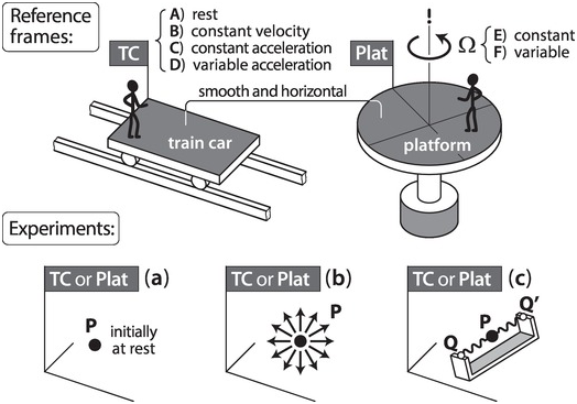
(a) Particle P is initially at rest on a small smooth horizontal surface (whose area is much smaller than that of the Earth) close to the Earth’s surface (Fig. 1.1a). If we consider only the horizontal motion (thus reducing the problem from 3D to 2D), the absence of roughness is equivalent to zero horizontal interaction, and P behaves as a free particle.
(b) Particle P is initially launched with a given speed in any horizontal direction and from any location on a smooth horizontal surface close to the Earth’s surface (Fig. 1.1b). Under these circumstances, P is again a free particle.
(c) Particle P is in a smooth slot in a support and attached to two identical springs with ends fixed to that support (Fig. 1.1c). If we consider only the rectilinear motion in the slot, the particle and the springs constitute the interacting system. The support will be glued anywhere and with any orientation on a horizontal surface close to the Earth’s surface.
In situations (1) and (2), we want to observe the evolution of the initial state (initial position and velocity of the particle). In situation (3) we will be interested in the equilibrium position of the particle.
The reference frame will be that of the smooth surface (which coincides with the springs support in the third situation). Let’s consider different choices:
A. Reference frame at rest with respect to the Earth.
B. Reference frame with a uniform rectilinear motion with respect to the Earth.
C. Reference frame with a rectilinear motion with constant acceleration with respect to the Earth.
D. Reference frame with a rectilinear motion with variable acceleration with respect to the Earth.
E. Reference frame rotating with constant angular velocity about a fixed axis with respect to the Earth.
F. Reference frame rotating with variable angular velocity about a fixed axis with respect to the Earth.
The reference frames A to D can be pictured as a train car with different motions on a horizontal straight railway, while the reference frames E and F can be assimilated to a platform rotating about an Earth-fixed axis.
Train cars and rotating platforms are observation reference frames familiar enough to the reader, so that the result of those three thought experiments can be correctly guessed. For instance, leaving the particle P at rest on a train car in different positions will have no consequences, whereas the time instant when this is done does have an influence on the observations when the train car has a variable velocity relative to the Earth. However, when leaving P at rest on a rotating platform, different initial positions yield different results: for instance, if located just on the platform center, the particle stays at rest.
Table 1.1 summarizes the influence of position, orientation and time instant for experiments (1), (2), and (3) in reference frames A to F. A “YES” means that at least one of the experiments does show a dependence on position/orientation/time instant.◄

Example 1.1 suggests that there are reference frames (A and B) which do not have any influence on the motion of particles because, as far as mechanical phenomena are concerned:
Those reference are called inertial or Galilean reference frames.
Example 1.1 also suggests the existence of reference frames (C to F) where some of those properties are not fulfilled: those are non-inertial or non-Galilean reference frames.
The formulation of the dynamics of a mechanical system will be simpler in a Galilean reference frame because it will have to take into account just the interactions between material objects (which will not depend on location, orientation, and time instant). However, proving the existence of at least one Galilean reference frame is strictly impossible, hence it is taken as a principle: the principle of existence of a Galilean reference frame.Footnote 3
1.3 Dynamics of a Free Particle: Newton’s First Law (Principle of Inertia)
The simplest dynamical problem is that of a free particle (a particle free from interactions) observed from a Galilean reference frame. A free particle is an idealization: all real particles interact with other material objects located at a finite distance from them. Solving the dynamics of a free particle amounts to a thought experiment, but it is an interesting and useful one.
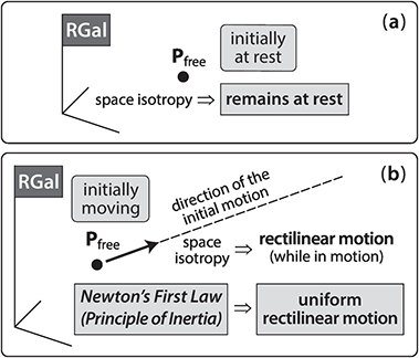
The properties of space and time in a Galilean reference frame partially restrict the possible motions of a free particle. If it is initially at rest, it will remain at rest (Fig. 1.2a): not doing so would imply choosing a direction for the initial motion, and that would contradict the isotropy of space. If its initial velocity is nonzero, its motion will have to be rectilinear (if it does not stop) though not necessarily uniform (Fig. 1.2b), as a curvature in its trajectory would again imply choosing a direction (the intrinsic normal direction). Summarizing: the properties of space and time in a Galilean reference frame (RGal) restrict the possible motion of the free particle according to  .
.
However, those properties do not imply that  . The particle could either increase or decrease its speed or even stop without contradicting any of them: this would be equivalent to imagine that space has a constant intrinsic friction equal in all locations and directions.
Stating that  , then, is formulating a principle (or a law): Newton’s first law (principle of inertia). That principle is usually expressed mathematically as
 (1.1)
(1.1)This law is based on everyday experience, and had already been formulated (among others, by Galileo): if there are no interactions, rectilinear motion with constant speed lasts forever (Fig. 1.2b).
The analytical expression of Newton’s first law (Eq. (1.1)) shows that there is an infinite number of Galilean reference frames (provided that we accept the principle of existence of one Galilean reference frame): all those having a uniform translation relative to the postulated one. The proof is straightforward through a composition of accelerations: between any of those reference frames and the initial one, the transportation and the Coriolis accelerations are zero.
1.4 Dynamics of Interacting Particles
Galileo’s Principle of Relativity
We have just proved that all Galilean reference frames share the law governing the dynamics of a free particle.Footnote 4 When seeking for the law governing the dynamics of interacting particles, a logical question is: Will the Galilean reference frames also share that law? Answering that question is equivalent to establishing a principle of relativity (a principle defining the set of reference frames for which a scientific law is valid).
In Newtonian mechanics, that principle is the special principle of relativity, also known as Galileo’s principle of relativity, as it was first enunciated by Galileo in 1632. A modern formulation of that principle is: The laws governing all mechanical phenomena are the same in all reference frames where the Newton’s first law is fulfilled. A consequence of that principle is that Galilean reference frames are not distinguishable through mechanical observations.Footnote 5
Mach’s Empirical Propositions
Though the vector formulation of dynamics proposed by Newton is the most widespread one and its application is certainly more straightforward (as interaction forces are a more practical representation of interactions than interaction accelerations because of their symmetry, as will be seen later on), it has many drawbacks from an axiomatic point of view. It relies on the concepts mass and force, but the definition of the former is unclear and that of the latter is actually implicit.
The two axioms introduced so far (Newton’s first law and the principle of relativity) do not mention mass or force, while Newton’s second and third laws do explicitly include these concepts. Mach’s formulation relies exclusively on interaction accelerations, and for this reason it will be presented before completing Newton’s axioms.
Ernst Mach’s axiomatization is based on three empirical propositions and two definitions. It is an alternative formulation whose application is not straightforward, but it has two important advantages:
it is based on accelerations, which are observable (and measurable) variables, and for that reason they correspond to “real” concepts;
it allows us to define in a rigorous way mass and force.
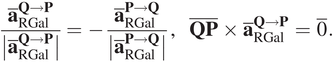
The first empirical proposition considers two isolated interacting particles P and Q. If observed from a Galilean reference frame, their accelerations will be exclusively the consequence of their mutual interaction. If  and
and  are the acceleration of P under the action of Q and that of Q under the action of P, respectively, the proposition states that those accelerations will be either attractive or repulsive, in the direction of
  (Fig. 1.3). Mathematically, this can be expressed as
 (1.2)
(1.2)This proposition is followed by the definition of inertial mass-ratio of two particles  :
:
 (1.3)
(1.3)If we choose a particular value  for a particle, the mass of the other particles may be determined straightaway.
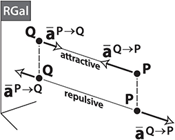
Equation (1.3) provides an interpretation for the inertial mass. As the product  is equal to
  , it follows that the particle which acquires a higher acceleration has a lower mass, and vice versa. Hence, the inertial mass is a measure of the resistance of a particle to change its state of motion.
The second empirical proposition is a principle of separation, and it guarantees that the determination of the ratio between the interaction accelerations of any pair of isolated particles (hence that of the mass-ratios) is unique through two statements:
A. the acceleration-ratio associated with a pair of particles is constant and independent from the interaction phenomenon
 (1.4)
(1.4)B. the acceleration-ratio is separable, that is, it can be expressed as the product of two independent acceleration-ratios.

This last idea is illustrated in Fig. 1.4 and can be formulated mathematically as:
 (1.5)
(1.5)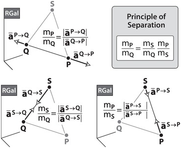
The third empirical proposition states that the accelerations that any number of particles (Q, S, T…) induce in a particle P are independent from each other. It is actually a principle of superposition, it is illustrated in Fig. 1.5 and can be formulated mathematically as:
 (1.6)
(1.6)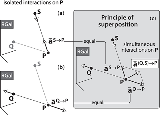
The combination between the principle of separation and the principle of superposition for the interaction accelerations yields a principle of superposition for the mass of particles. If QP is the particle obtained when P and Q share the same location (two dimensionless particles become one single particle in that case), its mass is the addition of those of P and Q:  .
.
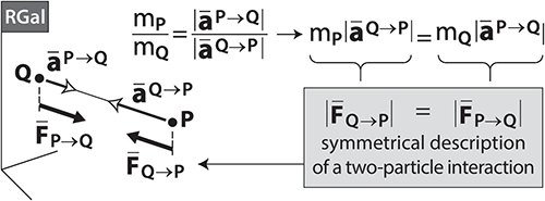
Finally, Mach introduces the concept of interaction force through a definition:
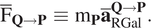 (1.7)
(1.7)The definition of interaction force is extremely useful: It describes the interaction between two particles through just one single magnitude  . This is not possible when we use accelerations as main magnitude to describe that interaction: as the interacting particles acquire different accelerations
  , we require two related magnitudes for a complete description (Fig. 1.6).
1.5 Closing the Formulation of Dynamics: From Mach’s Axiomatics to Newton’s Laws, and Principle of Determinacy
Newton’s laws of motion can be derived from Mach’s propositions and definitions.
Newton’s Third Law
The first empirical proposition (Eq. (1.2)) and the definition of force (Eq. (1.7)) lead to:
 (1.8)
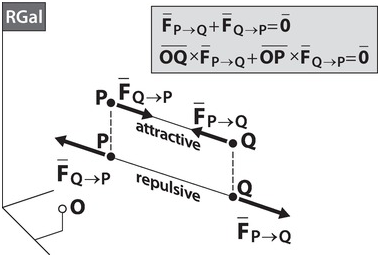
(1.8)which is Newton’s third law (principle of action and reaction). Note that the interaction forces between P and Q fulfill:
 (1.9)
(1.9)where O is any point. The cross product  defines the moment (or torque)
  of force
  about point O. Equations (1.9) show that the resultant force and the resultant moment (about any point O) of an action–reaction pair of forces are always a zero (Fig. 1.7).
Newton’s third law provides powerful information about the interaction force between two particles, and it is considered as the main law by many authors precisely because it introduces the symmetry in the description of the interaction mentioned earlier (description of the interaction through one single magnitude).
Newton’s Second Law
The definition of force (Eq. (1.7)) together with Mach’s third empirical proposition (superposition principle, Eq. (1.6)) lead to:
 (1.10)
which is Newton’s second law (fundamental law of dynamics).Footnote 6 This formulation contains a principle of superposition for the interaction forces.
Principle of Determinacy
Whether we adopt Newton’s or Mach’s axiomatics, the principle of determinacy has to be added to the other laws to complete the formulation of dynamics. It is actually known as the Newtonian principle of determinacy, though he did not postulate it as a law but commented on it as an observation. A possible formulation is: “In an isolated system (undergoing no other interactions but those between the system’s particles), the particles’ accelerations at each time instant depend exclusively on the system’s mechanical state (position and velocity of every particle) at that same time instant.”Footnote 7 In other words, the initial mechanical state determines univocally its future evolution. Hence, this principle states that isolated mechanical systems have no memory.
This principle may seem incompatible with everyday experiences, such as driving a vehicle, because it is without discussion that its future evolution depends on the driver and not on the present mechanical state. However, driving a vehicle (or controlling a system, in general) consists basically of varying the interactions – internal and external – acting on the system.Footnote 8 It may also seem incompatible with the existence of “memory” materials capable of recovering past shapes, but we must keep in mind that those are very complex systems – with interactions between deformable bodies – whose mechanical description is usually over-simplified.
1.6 Usual Galilean Reference Frames
We have defined the Galilean reference frames in three different ways:
those where space is homogeneous and isotropic, and time is uniform;
those where the law of inertia is fulfilled;
those where Newton’s second law is fulfilled.
Checking the first two conditions is impossible, but the third condition provides a practical check: when studying a particular problem, a reference frame can be considered to be Galilean if Newton’s second law is fulfilled within the degree of accuracy sought for in that problem (that is, if the measured acceleration can be justified exclusively from interaction forces within that degree of accuracy). Hence, accepting whether a reference frame is Galilean is directly associated with the degree of accuracy of the calculations. The following reference frames are taken as Galilean ones in different fields of application.
Terrestrial reference frame (TRF): In short, it is the Earth reference frame. It can be considered as a Galilean one for the usual short-range applications of mechanical engineering: machines, ground vehicles… However, astronautical applications (such as the motion of artificial Earth satellites) and other medium-range phenomena reveal its non-Galilean characteristics: The rotation motion of cyclones and anticyclones, the rotation of the plane of oscillation of Foucault’s pendulum, the eastward deviation of projectiles launched to the north/south from the north/south hemisphere, the eastward deviation of objects falling to the ground… Appendix 1B quantifies the non-Galilean characteristics of the TRF.
Conventional celestial reference frame (CCRF): It contains the Earth’s center of mass and does not rotate with respect to the distant galaxies (or fixed stars). Relative to the CCRF, the Earth rotates about its axis with a constant angular velocity of one turn per sidereal day, which is the time needed by the Earth to complete one turn relative to the distant galaxies (Appendix 1B).
The CCRF is an acceptable Galilean reference frame in a first approximation for the astronautics of artificial Earth satellites and for the medium-range phenomena listed in the TRF comments, but not when studying tides and astronautics of flights to the Moon and the planets.
International celestial reference frame (ICRF): It is an astronomical reference frame. It contains the solar system barycenter and does not rotate with respect to the distant galaxies. It is the usual Galilean reference frame in astronomy and astronautics. With respect to the ICRF, the Earth rotates about its axis with a constant angular velocity of one turn per sidereal day, and its center of mass describes an elliptic orbit (slightly disturbed by the gravitational attraction of the Moon and the planets) with the Sun as one of its foci.
The International Astronomical Union (IAU) is in charge of the redefinition of the standard astronomical reference frame (SARF) according to modern high-precision measurements. As far as Newtonian mechanics is concerned, there is no need for a more precise definition: The accuracy of the results obtained under the hypothesis of the ICRF as a Galilean reference frame is comparable to that of the Newtonian approach.
1.7 Interaction Forces between Particles: Kinematic Dependency
The fundamental equation of dynamics (Newton’s second law, Eq. (1.10) may be used to predict the acceleration of a particle P from the interaction forces  exerted on it (direct dynamics), or to find out what forces would be required to obtain a prescribed motion for P (inverse dynamics). In the context of engineering, inverse problems in dynamics are associated with the use of actuators in mechanical systems. The forces that actuators may introduce between their endpoints to guarantee a given motion may be an unknown of the problem.
Among the other interaction forces, many of them may be formulated: their value can be obtained through a mathematical equation (formula) known before solving the problem. As the unknown in the fundamental equation is the acceleration, those forces may depend on the position and velocity of the interacting particles. However, that dependency has to be consistent with all principles and laws of Newtonian dynamics.
Any formulation we provide will have to include parameters: from the dimensional point of view, positions [length] and velocity [length/time] cannot yield the dimensions of the right-hand side of Eq. (1.10). The uniformity of time in Galilean reference frames restricts those parameters to constant ones. In other words: that principle forbids any time-dependent formulation of interaction forces.
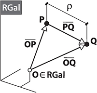
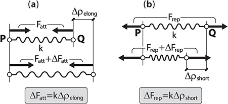
Restrictions on the Position Dependency (Fig. 1.8)
Because of the homogeneity of space in Galilean reference frames, the dependence of
on the positions of P and Q cannot be through all the information contained in their position vectors and , but just through their difference .Isotropy does not allow a dependency on a particular direction. Thus, only the distance
is acceptable in the formulation of .Because of the principle of determinacy, the value of
at any time instant may only depend on that of at that same time instant.


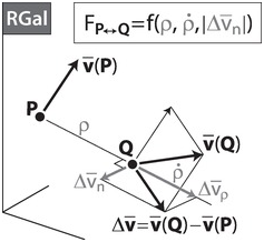
Restrictions on the Velocity Dependency (Fig. 1.9)
Because of Galileo’s principle of relativity, the dependence of
on the velocities of P and Q cannot be through all the information contained in the vectors and separately, but just through their difference:In general, that difference will have a component parallel to the line
and another one perpendicular to that line: .Isotropy does not allow a dependency on a particular direction not associated to the existence of the two interacting particles. Isotropy restricts the type of dependence of
on . The interaction force may depend on the value of (that is, on , where and describe the separating and the approaching velocity of particles P and Q, respectively), and on just the magnitude of (though usual formulations do not depend on that component).Because of the principle of determinacy, the value of
at any time instant may only depend on those of and at that same time instant.


Summarizing:  . Note that the values
  are the same in all reference frames (whether Galilean or not), whereas
  is the same only in Galilean reference frames but may change when moving to a non-Galilean one. Hence, the formulation of any interaction depending exclusively on
  and
and  will be shared by all reference frames.
The usual interactions in mechanical systems do not depend on  . Therefore, only formulations depending on
  and
and  will be considered from now on.
1.8 Contact Forces between Particles and Extended Bodies
So far, we have been considering action–reaction forces between pairs of particles P and Q. However, the problems found in mechanical engineering do not deal with dimensionless particles but with extended bodies. The action–reaction forces have to be understood as interactions between particles belonging to different extended bodies, and this allows us to consider contact interactions. Those interactions are strictly impossible between a pair of dimensionless particles P and Q: if in contact, they would become one single particle.
Contact forces come from the local deformations of the objects in the vicinity of the contact points. Those deformations are accurately formulated in solid mechanics, but they cannot be dealt with when objects are modeled as rigid bodies: rigid bodies do not deform, they are impenetrable.
The modeling of those forces is not possible: consistency with the previous section leads to the conclusion that they cannot be formulated, and their value becomes an unknown of the dynamical problem.
Among the contact interactions, there is a subset whose value adapts in order to guarantee a kinematic restriction. They are the so-called constraint forces, and their value at every time instant is calculated through Newton’s second law. The number of independent components (in the three directions of space), however, can be predicted beforehand from the kinematic restriction they are associated with. The description of those components is the characterization of the constraint force.
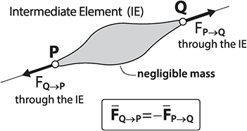
Constraint action–reaction pairs can also appear between particles at a finite distance  , provided there is an intermediate element with negligible mass between them guaranteeing a restriction on
  .
.
1.9 Formulation of Interaction Forces
The gravitational attraction was the first interaction to be formulated. Though not very intense, it is an infinite-range interaction, and it is the only one that matters when studying the motion of celestial objects (such as planets and stars).
Newton formulated the law of universal gravitation at the same time he proposed his three laws. The four laws were based on an important amount of empirical quantitative data (collected mainly by Tycho Brahe) on the motion of the planets and their synthetic kinematical description relative to a heliocentric reference frame given by Kepler’s laws. In short: The planets’ acceleration pointed toward the Sun and was inversely proportional to the distance squared between planet and Sun.
Gravitation has a particular status among the interactions considered in engineering mechanics. On the one hand, it is one of the so-called fundamental interactions in physics: It is not the result of any underlying phenomena which combine and yield that interaction; in other words, its formulation is not phenomenological.
On the other hand, it is the only interaction “at a distance” (that is, between particles separated in space without any intermediate element connecting them). All other interactions between particles that will be formulated in this section call for intermediate elements: elements connected to those particles and whose mass is significatively smaller than that of the particles. In a first approach, then, the mass of those elements can be neglected, and the force exerted by one particle at the endpoint of the element is equal, though with opposite sign, to that exerted by the other particle at the other endpoint. In other words, those two forces fulfill Newton’s third law, and can be understood as an action–reaction pair of forces between the particles (Fig. 1.10).
The usual intermediate elements found in mechanical systems are springs, dampers, and linear actuators. Interactions between particles through those elements are the result of underlying phenomena whose overall effect on the particles is formulated at a phenomenological level through empirical models.
Gravitational Force
Newton’s law of universal gravitation states that two particles P and Q attract each other with a force directly proportional to the product of their masses and inversely proportional to  (Fig. 1.11):
 (1.11)
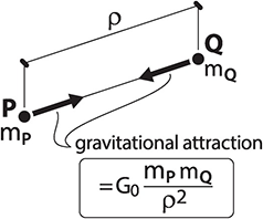
Strictly speaking,  and
and  in Eq. (1.11) are the gravitational masses of the particles. They are conceptually different from the inertial masses, but there is no empirical evidence so far that they should differ, so they will be treated as one same thing. The constant parameter
  in Eq. (1.11) is the universal constant of gravitation
  in the International System of Units, SI), and is independent from the particles (that is why it is a universal constant).Footnote 9
The vector  is called the gravitational field
  created by P at Q location. Appendix 1.A presents the formulation of the Earth’s gravitational field.
The universal law of gravitation has been widely discussed because of some very particular features. On the one hand, and as a result of the identification of inertial mass and gravitational mass, it predicts a same acceleration (relative to a Galilean reference frame) for any particle under the same gravitational field. On the other hand, Eq. (1.11) describes an instantaneous interaction. The direction and intensity of the gravitational attraction is adjusted instantaneously whatever the distance between the interacting particles might be: the gravitational field propagates with an infinite speed!Footnote 10
Interaction Force through Springs
The term spring is used to designate any element with negligible mass responsible for an interaction force depending exclusively on the distance between particles (called “spring length” from now on):  . Springs may introduce either an attraction or a repulsion between their endpoints.
The most usual case is the linear spring, where the force change associated with a change of spring length is proportional to that length change through a constant parameter called the spring constant k:
 (1.12)
Springs constants are always positive. However, the term spring may be used in a more general sense for any physical phenomenon whose net force is a function of  (in this context, the gravitational force can be seen as a spring). In that case, we will talk of equivalent spring, and the constant may be negative.
A real spring (not an equivalent one) has a nonzero slack length  (length for which the force between the spring endpoints is zero). From that state, the spring will generate an attraction force if the length is increased
  and a repulsion force if it is decreased
  .
.
The force associated with a spring within a mechanical system may evolve from attraction to repulsion with time. When solving the system dynamics, the spring force is drawn either as an attraction or a repulsion, and its value is formulated accordingly (Fig. 1.12).
If the spring force is formulated from a nonzero-tension state (a state where its length  is higher or lower than
  , and the spring force is
  ), the choice of its description as an attraction or a repulsion is made according to the nature of the initial force
  :
:
 (1.13)
In the context of a particular problem, the spring length has to be expressed as a function of the generalized coordinates  describing the system configuration.
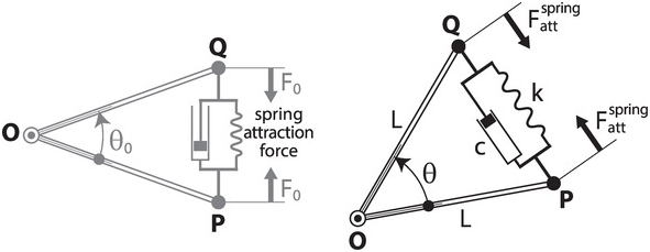
► Example 1.2
The linear spring connecting the endpoints of two bars articulated at point O has a constant k and exerts an attraction force  between P and Q when
  (
(
). For any  value, then, the spring force is formulated as an attraction force:

◄
► Example 1.3
The hydraulic cylinder prescribes a motion  , and the angular coordinate
  evolves dynamically. When
  and
and  , the spring is compressed and exerts a force
  between its endpoints (Fig. 1.14).
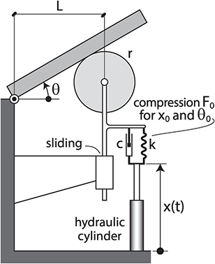
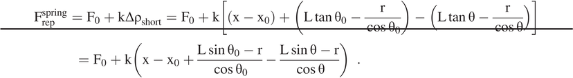
As the initial force  is a repulsion, the spring force for any configuration will be formulated as a repulsion force:
◄
In a nonlinear spring, the force change is not proportional to the spring length change (Fig. 1.15).
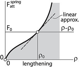
For small length changes around a given length  , the spring force may be approximated through a Taylor series up to the linear term:
 (1.14)
The derivative  can be understood as the constant of an equivalent linear spring for lengths close to
  .
.
Interaction Force through Dampers
Dampers with negligible mass exert a force opposite to the approaching or separating velocity between their endpoints. The force value depends on that velocity, and sometimes also on the distance  between those points:
  .
.
The most usual case is the linear damper (or viscous friction damper). In those dampers, the force is strictly proportional to  through the damper constant, c. As in springs, the damper force may be an attraction or a repulsion. When the damper is assembled in parallel with a spring (spring–damper system), the criterion to draw and formulate that force is the same as that chosen for the spring:
 (1.15)
► Example 1.5
The repulsion force exerted by the damper in Example 1.3 is

Actually, the distance between the damper endpoints is  plus a constant value, but that constant can be omitted because its time derivative is zero.◄
Interaction Force through Actuators
An actuator (or driver) is an element able to produce a prescribed motion or a prescribed interaction according to a predefined time law. Its functioning requires a control system and an energy source.
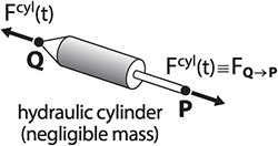
The most usual actuator between pairs of particles P and Q is the hydraulic cylinder. As with springs and dampers, the effect it has on P and Q is described as an action–reaction pair of forces when its mass is negligible (Fig. 1.16). The force  it introduces can either be a prescribed function or an unknown whose evolution has to be adjusted in order to guarantee a prescribed motion
  .Footnote 11
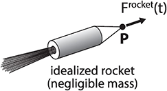
A rocket with negligible mass can be considered as an idealized actuator. It is an interesting case as it seems to be using just one force of the action–reaction pair to control the motion of a particle P (Fig. 1.17). This is not so: the reaction force is applied to the high-speed gas particles ejected by the rocket in a direction opposite to  .
.
1.10 Characterization and Limit Conditions of Constraint Forces: Friction Forces
The forces associated with the contact of a particle P and an extended rigid body are the consequence of two main features of rigid objects: impenetrability and roughness (that generates friction). They both may restrict the possible motion of P relative to the rigid body.
Particle–Surface Interaction: Force Associated with Impenetrability
The impenetrability of a rigid body S forbids the normal approaching velocity of a particle P relative to it when they are in contact:  . It is a unilateral restriction, as the separating normal motion is not restricted.
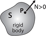
The kinematic constraint  translates into a repulsion normal force N on P that takes the value required to guarantee that constraint (Fig. 1.18). If that force did not exist, other interaction forces on the particle could provoke a penetration of P into the rigid body. As it is a unilateral constraint, the value of N has to be strictly positive.
The constraint normal force can be formulated as a function of the normal deformation of objects. When that deformation is neglected (hypothesis of rigid body), that force cannot be formulated, and it becomes an unknown of the dynamical problem.
In unilateral normal forces, a zero value  indicates that the contact is about to be lost. When the N value required to maintain that contact is negative
  , the contact is lost and a separating normal motion is actually taking place.
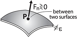
If the particle P motion is restricted by two close surfaces, we say that there is a bilateral constraint (Fig. 1.19). As an adimensional particle cannot be simultaneously in contact with two surfaces, we will assume an infinitesimal mutual separation  between them, and P will be either in contact with one surface or the other. In that case, the normal force on P may have either sign.
► Example 1.6
The particle P is initially at rest relative to a curved ground (Fig. 1.20a). The normal force on P compensates the weight (otherwise P would penetrate the ground).
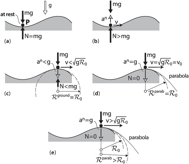
If P slides on the ground with speed v (Fig. 1.20b), the value of the normal force is not the same. The normal acceleration of P relative to the ground is upward, thus N has to compensate the weight and provide that acceleration:  .
.
When P reaches the highest position (Fig. 1.20c), its normal acceleration relative to the ground is downward, so  . If the ground radius of curvature at that location is
  and the speed value is
  , the normal acceleration is
  . As
. As  and
and  , the weight compensates the normal force and provides that acceleration.
If P goes through that position with speed  such that
  , the normal force is zero, and that indicates that the ground contact is about to be lost. The curvature radius of the P trajectory is not imposed by the ground curvature but by the speed value and the weight (Fig. 1.20e).
If  , the weight will be responsible for a parabolic trajectory with
  ,and there will be no ground contact (Fig. 1.20e).◄
Particle–Surface Interaction: Force Associated with Friction
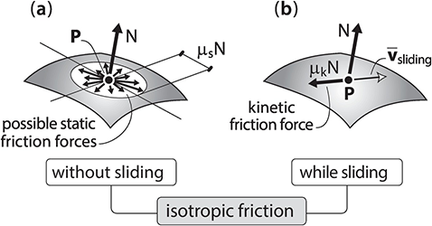
The roughness of a rigid surface S is responsible for a tangential force (or friction force)  on the particle P when they are in contact.Footnote 12 When there is sliding between P and S (that is, when
  , so there is no kinematic restriction in that direction), that force is called dynamic or kinetic friction,Footnote 13 it is opposed to the sliding velocity when the roughness is isotropic, and it may be formulated as a function of that velocity.
When there is no relative sliding, the tangential force is called static friction, and it is a constraint force: its value adapts in order to keep the kinematic restriction  . That force can be modeled as a function of the tangential deformation of objects. When that deformation is neglected (hypothesis of rigid body), that force cannot be modeled: it is an unknown of the dynamical problem.
When there is no lubricant between the particle and the surface, Coulomb’s law of friction (or dry friction model) provides the simplest description for that phenomenon. If the roughness is isotropic:
The static friction force
may have any direction and may take any value within the range in order to guarantee the no-sliding restriction (Fig. 1.21a). The adimmensional constant coefficient is called static friction coefficient. When the friction force required to maintain the kinematical constraint is , the particle slides and becomes a kinetic friction force.The kinetic friction force
is opposed to the sliding velocity, and its value is (Fig. 1.21b). The adimmensional coefficient is the kinetic friction coefficient, and it is assumed to be constant.Footnote 14 Usually .


Friction in materials with anisotropic roughness may be modeled through direction-dependent friction coefficients. For the particular case of orthotropic surfaces (with different properties along two orthogonal directions), two different friction coefficients  describe the phenomenon. The allowed range of values for
  is
is  , where
  , and the direction of
  is not any more opposed to the sliding velocity.
When one of the two friction coefficients is much lower than the other  , a first approximation with
  yields a simpler model.
When there is lubricant between the particle and the surface  , the kinetic friction force can be formulated as a viscous friction proportional to the sliding velocity:
  . The coefficient c may be a function of the normal constraint force.
Particle–Curve Interaction
The interaction between a rigid curve and a particle P moving along it can be visualized either as that of a small hollow sphere pierced by a thin wire (Fig. 1.22a), or a particle moving in a tube with an infinitesimal diameter  (Fig. 1.22b). In both cases, we will consider that P is in contact with just one side of the wire or the tube (as was assumed earlier in particles constrained by two close surfaces), hence the normal force N on P will have any direction on the plane perpendicular to the curve (Fig. 1.22c).
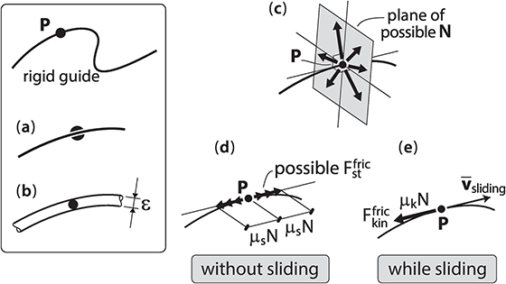
The friction force between curve and particle may be modeled through Coulomb’s friction law (Fig. 1.22d,e).
Constraints between Particles through Intermediate Elements
Two different constraint forces have been introduced so far: the normal force and the static friction force associated with a single-point contact between a particle and a surface or a curve force. Following what has been done to introduce interactions “at a distance” between particles through springs, dampers, and actuators, we will consider now the possibility of constraints “at a distance” between particles through intermediate elements with negligible mass.
Constraints between two particles P and Q can be introduced through rigid thin bars and through inextensible threads. A rigid bar between P and Q generates a bilateral constraint preventing the particles to approach or separate:  (Fig. 1.23a). That kinematical restriction translates into a pair of repulsion or attraction forces, respectively.
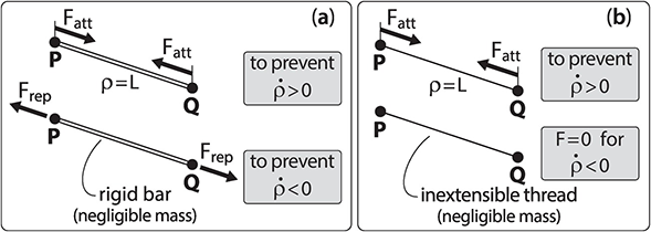
An inextensible thread under tension between P and Q generates a unilateral constraint preventing just the separation velocity between them, as the thread length cannot increase (Fig. 1.23b). Hence, a tensioned thread can only transmit attraction forces between P and Q.
Analytical Characterization of Constraint Forces
The previous description of the constraint forces of a rigid body S on a particle P relies on the description of the kinematical restrictions they are supposed to guarantee. Mathematically, this can be expressed as an orthogonality between the force and the particle allowed motion:
 (1.16)
The description of the velocity of P has to be done from the S reference frame. Eq. (1.16) is the equation for the straightforward analytical characterization of single-point constraint forces. Note that there is a one-to-one correspondence between the nonzero components in  and the zero components in
  .
.
When the constraint force on P comes from another particle Q through an intermediate element, the kinematic description has to be done on any reference frame R where  .
.
Characterizing constraint forces and calculating them are two different things. The former consists on assessing the possibility of existence of those forces, and it does not depend on the actual motion of the constraining elements (the rigid body S or the particle Q). Calculating the constraint forces (finding out their values) requires the application of the laws of dynamics, and the result does depend on the actual motion of the particle and the constraining elements.
1.11 Dynamics in Non-Galilean Reference Frames: Inertial Forces
Non-Galilean reference frames move with an accelerated translational motion or a rotational motion relative to Galilean ones. The formulation of dynamics in those reference frames is more complicated than in Galilean ones because space and time do not fulfill some or all the three properties mentioned in Section 1.2 (homogeneity, isotropy, uniformity). Hence, besides the interaction forces between particles, that formulation includes terms (called inertial forces) which are location-, orientation- or time- dependent:
 (1.17)
The acceleration  can be obtained from
  through a composition of accelerations.Footnote 15 If the Galilean reference frame is the absolute (AB) frame, and the non-Galilean one is the relative (REL) frame:
 (1.18)
Combining Eq. (1.18) with Newton’s second law (Eq. (1.10)) yields:
 (1.19)
where  and
and  are the transportation inertial force and the Coriolis inertial force, respectively.
The transportation force and the Coriolis force are proportional to the particle mass (as the gravitational force). The transportation force is location dependent, while the Coriolis force is velocity dependent. Both forces may depend on singular directions and may vary along time (different time instants are not equivalent). The lack of space homogeneity or isotropy, or of time uniformity, found in some of the reference frames presented in Example 1.1 comes from the transportation or the Coriolis forces that have to be taken into account in those reference frames.
Coriolis forces become zero in static situations (no motion relative to the non-Galilean reference frame), but transportation forces persist. For this reason, we develop a certain intuitive knowledge concerning the latter. By way of an example, let’s consider a vehicle accelerating (braking) on a straight road: the car passengers undergo the effect of the transportation forces (associated with the chassis reference frame) pushing them backward (forward). In cornering conditions, the passengers are pushed to the outer side of the road by the centrifugal transportation force.
That intuition may be misleading: it may seem that the transportation forces are actually associated with being at rest relative to the reference frame, and that the passenger motion tendency is actually the result of being “physically” transported by the reference frame.
In general, we are less aware of the Coriolis forces, as they add up to the transportation ones (when we are moving relative to the non-Galilean reference frame). As they are perpendicular to the our relative motion (such as  ), they do not modify the relative speed.
Relationship between Inertial Forces Associated with Non-Galilean Reference Frames with a Relative Translational Motion
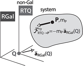
As for particles, the dynamics of rigid bodies may be formulated in Galilean or non-Galilean reference frames. However, once an initial choice of reference frame has been made, one may realize that the calculation of some magnitudes (such as angular momentum, as will be seen in Chapter 4) may be simpler in a frame with a translational motion (not necessarily rectilinear and uniform) relative to the initial frame. The formulation of the theorems in the new frame is not complicated, and overall that second choice may be advantageous. As that new frame does not rotate relative to the initial one, it will be described as the “Reference frame with a Translational motion and moving along with point Q”: RTQ in short. Whenever that RTQ is not Galilean, the inertial forces on each point of the rigid body have to be taken into account.
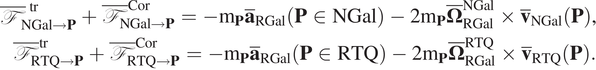
If the first reference frame is Galilean, only transportation forces will have to be considered in the RTQ  . As all points in the RTQ have exactly the same motion relative to Gal, the field of inertial forces acting on a system of particles will be uniform and proportional to the particle masses (Fig. 1.24).
If the first reference frame is non-Galilean, both the transportation and the Coriolis inertial forces  and
and  have to be taken into account in general even if we do not move relative to the RTQ. They are associated with
  and
and  (Fig. 1.25a).
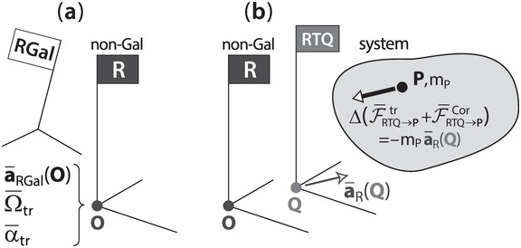
If we move to the RTQ, the new inertial forces  and
and  will be different. It is always possible to calculate them from
  and
and  , but they can be obtained from
  and
and  in a very straightforward way just by adding one term (Fig. 1.25b):
 (1.20)
The additional term that has to be added when moving to the RTQ corresponds to a uniform force field associated with the transportation force on Q that would have been required if R were Galilean.
♣ Proof
The inertial forces on P associated with the NGal and the RTQ reference frames are:
Taking into account that the RTQ does not rotate relative to the NGal  , and that

the difference between the inertial forces in those two reference frames becomes:

♣
1.12 Examples
► Example 1.7
A particle P with mass  describes a circular trajectory with center O, radius R, and constant speed
  on smooth horizontal ground. P is attached to O through an inextensible thread.
The thread tension T can be calculated through Newton’s second law formulated in the Galilean ground reference frame E (Fig. 1.26a). As the acceleration of P is centripetal with magnitude  , it requires a centripetal force with value
  which is provided exclusively by the thread (as the ground is smooth).
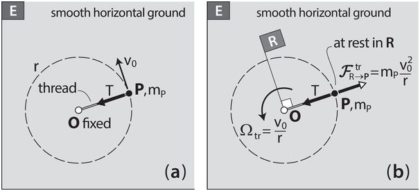
The same result can be obtained with Newton’s second law formulated in the non-Galilean reference frame R that rotates with angular velocity  relative to the ground (Fig. 1.26b).
The particle is permanently at rest in R, so the zero net force on P has to be zero:

Here,  because
  , and the transportation inertial force is
  , centrifugal with value
  . Hence, the thread tension has to compensate
  , so it is centripetal with that same value.
The comparison between the dynamical interpretations in these two reference frames is interesting:
In the rotating frame R, there is static equilibrium, and the thread tension equilibrates the centrifugal force associated with the non-Galilean behaviour of R.
In the ground reference frame E there is no static equilibrium, and the acceleration has to be provided by the thread tension.◄
► Example 1.8
A particle P with mass  slides along a smooth circular wire located on a vertical plane that rotates with constant angular velocity
  relative to the ground (Fig. 1.27a).
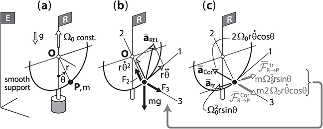
The equation of motion for the angular coordinate  that gives the location of P on the guide and the two components of the constraint force between guide and particle can be obtained through Newton’s second law formulated in the Galilean ground reference frame (E):

The first component is the equation of motion, and the other two yield the value of the constraint forces.
These results can be obtained through the application of Newton’s second law in the guide reference frame. As it is a non-Galilean reference frame, the transportation and the Coriolis forces will have to be included (Fig. 1.27b,c):

The equation  yields the same results.◄
► Example 1.9
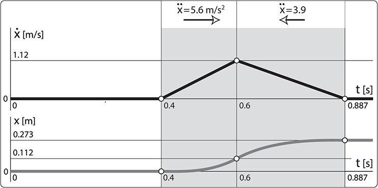
A particle P with mass  is initially at rest on a horizontal platform (vibrating feeder) which moves under the action of a hydraulic cylinder. That actuator prescribes the periodic speed
  relative to the ground E (Fig. 1.28). The friction coefficient between platform and particle is
  . Initially the particle is at rest relative to the platform.
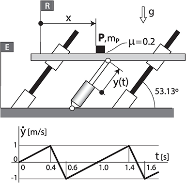
The interaction forces on P are the weight and those associated with the platform contact: a normal constraint force and a horizontal friction force. If P does not slide on the platform, the horizontal force is a static friction whose value is within the range  ; if it slides, it is a kinetic friction with value
  . In the present case,
If the dynamics of P is formulated in the platform reference frame R, the transportation force has to be added to the interaction forces:  . As the platform motion is along an oblique direction,
  will have two components.
As P is initially at rest on the platform  , the friction force is a static one. Figure 1.29a shows the forces per unit mass that have to be considered during the first phase. The static friction compensates the horizontal component of
  , so
, so  . The normal force compensates the weight plus the vertical component of
  , and its value is
  . As
. As  , no sliding appears during the first phase.
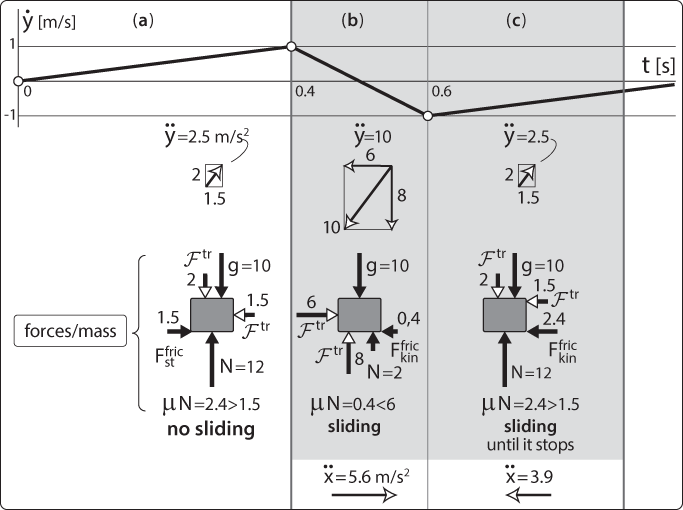
During the second phase (Fig. 1.29b), the normal force is lower and the maximum value of the friction force cannot compensate the horizontal inertial force, so sliding starts  .
.
In the third phase,  , so stiction can eventually happen. The two horizontal forces (inertial and dynamic friction) add up against the sliding (Fig. 1.29c). If they succeed in stopping it before the phase end, the nonsliding condition will be kept until the cycle
  restarts.
The time evolution of the velocity  and the position
  of P on the platform is shown in Fig. 1.30. A straightforward time integration of
  shows that sliding does stop before the cycle is over.◄