


1. Introduction
Remote sensing is a powerful tool that offers the ability to quantitatively examine the physical properties of snow in remote or otherwise inaccessible areas where measurements may be expensive and dangerous. Moreover, the global coverage and regular repeatability of measurements offered by satellite remote sensing allows scientists to monitor the vast temporal and spatial variability of snow cover. Satellite and airborne remote sensing augments the relatively sparse in situ observations, thereby affording important spatial context for such measurements. Routinely carried out since the 1960s, remote sensing of snow has created a multidecadal archive of variability and trends in snow cover. Innovations in sensor technology and digital image processing allow scientists to visualize and monitor snow cover for hydrology and water resources management, climatology and ecosystem science. Early work on remote sensing of snow and glaciers has been covered in the excellent review by Reference König, Winther and IsakssonKönig and others (2001) and the valuable text by Reference ReesRees (2006). Remote sensing of glaciers and ice sheets is rather extensive and beyond the scope of this paper. This review concentrates on recent advances in satellite, airborne and ground-based remote sensing of seasonal snow.
In many ways, the research questions involving seasonal snow have not changed over the past several decades since the inception of remote sensing. We still want to know the spatial extent of snow cover, snowpack properties such as grain size and albedo, snow depth, snow water equivalent, and the onset of snowmelt. However, the accuracy with which we can answer these questions has developed significantly. The following sections are arranged with regard to these questions, highlighting advances within the past decade.
2. Snow-Cover Extent
2.1. Binary classification of snow cover
The unique and spectrally varying reflectance of snow relative to other common earth surface materials forms the basis for mapping snow-covered area (SCA) from space. There are two main methods for mapping SCA: a binary classification in which each pixel in an image is designated as ‘snow’ or ‘non-snow’ or a fractional snow-cover classification in which the fraction of snow cover in an image pixel is computed. A multispectral binary classification was first developed by Reference DozierDozier (1989) with satellite data from the Landsat Thematic Mapper (TM), using a ratio of reflectance values in the visible and near-infrared wavelengths. This band ratio approach formed the basis for the widely used snow-cover mapping product for the Moderate Resolution Imaging Spectroradiometer (MODIS; Reference Hall, Riggs, Salomonson, DiGirolamo and BayrHall and others 2002; Reference Hall and RiggsHall and Riggs, 2007), which uses the normalized-differ- ence snow index (NDSI).
where ρ is the surface reflectance in MODIS bands 2 (0.841−0.876 μm), 4 (0.545−0.565 μm) and 5 (1.230−1.250 μm). One of the key difficulties in mapping snow- covered area is forest cover, which obscures snow beneath the canopy and also contributes to the overall pixel reflectance. Unlike earlier versions of this SCA mapping approach, the MODIS snow product incorporates an adjustment for snow in the presence of dense vegetation (Reference Klein, Hall and RiggsKlein and others, 1998). Using a combination of nor- malized-difference vegetation index (NDVI), NDSI and a reflectance threshold of 0.11 in MODIS band 4, the canopy adjustment reduces errors of omission and commission in snow-covered area mapping although the overall improvement was not strictly quantified. With the exception of very dense canopy or late-spring conditions, this canopy adjustment provides users with an estimate of snow cover in areas where vegetation may be obscuring the snow, an important consideration for seasonal snow cover in most areas except alpine and prairie regions. The MODIS binary snow-cover product agrees well with satellite-based snow- cover products and in situ measurements (Reference Klein and BarnettKlein and Barnett, 2003; Reference Maurer, Rhoads, Dubayah and LettenmaierMaurer and others, 2003; Reference Parajka and BlöschlParajka and Bloschl, 2006), with underestimation of ˜12% (typically, the low-elevation snow cover) and overestimation of ˜15% (typically, the higher-elevation snow cover) (Reference Klein and BarnettKlein and Barnett, 2003; Reference Parajka and BlöschlParajka and Bloschl, 2006).
An interesting application of the NDSI is shown in the work of Reference Kolberg and GottschalkKolberg and Gottschalk (2010) in which they computed NDSI from MODIS surface reflectance data over a large region in Norway. They developed snow depletion curves using Bayesian analysis of 6 years of NDSI data during the ablation period over a large region in Norway. Their results show a significant reduction in the standard error of a precipitation-runoff model when using the NDSI- derived snow depletion curves.
2.2. Fractional snow-cover mapping
Fractional snow-covered area is the viewable fraction of snow cover in a pixel. It has values ranging from 0.0 to 1.0. The fractional area is often preferred over the binary classification because it can more accurately account for snow-cover variability in areas that have patchy snow such as near the snow line and in wind-scoured areas.
2.2.1. Fractional snow-cover mapping using NDSI
Reference Salomonson and AppelSalomonson and Appel (2004) developed a fractional snow- cover algorithm based on changes in the MODIS NDSI. They found that spatial mixtures of snow, vegetation and rock within a 500 m MODIS pixel reduce the NDSI value for that pixel. Using binary snow cover derived from 30 m Landsat Enhanced TM Plus (ETM+) data in bands 2 (0.52−60 μm) and 5 (1.55−1.75 μm) they empirically calibrated the changes in MODIS NDSI to create estimates of fractional snow-covered area. However, while the ETM+ bands are similar in spectral position to those of MODIS for use in the NDSI, the ETM+ bands have a much smaller radiometric dynamic range than MODIS, and band 2 often saturates over bright snow. Thus, an NDSI from ETM+ will have a different meaning than that derived from MODIS. The authors report a mean absolute error less than 0.1 for areas without vegetation cover. It should be noted that the statistical relationship between NDSI and snow-cover fraction exhibits a slope much greater than unity and substantial spread in the data cloud (see Reference Salomonson and AppelSalomonson and Appel, 2004, Fig. 4). This results in an extremely wide range of possible values of snow-cover fraction for a given value of NSDI. Even if it is a well-constrained relationship, the fractional snow-covered area in areas of forest canopy will be erroneously low because it is estimating only the viewable snow cover.
2.2.2. Fractional snow-cover mapping using spectral mixture analysis
The earliest method for mapping fractional snow-covered area used a linear spectral mixture analysis approach applied to hyperspectral imaging spectrometer data (Reference Nolin and DozierNolin and others, 1993). Regardless of whether hyperspectral or multispectral data are used, spectral mixture analysis requires that the sensor must be capable of detecting differences in the spectral reflectance characteristics of the various land-cover elements in the image such as snow, vegetation, rock/soil and open water. Each land-cover type can be represented by a reflectance ‘end-member’, which is the spectral reflectance of the most homogeneous example of that land-cover type in the image. For spectral mixture analysis, the sensor should have at least as many channels as end-members in the image, and the reflectance information recorded within each channel should contain unique (nonredundant) spectral reflectance values for each land-cover type (Reference Sabol, Adams and SmithSabol and others, 1992).
Spectral mixture analysis assumes that the reflectance of a pixel containing multiple end-members is assumed to be a linear mixture of the reflectance values of each end-member weighted by the end-member fraction in the pixel:

where ρi is the pixel reflectance in spectral band i, f is the fraction of the jth end-member in the mixed pixel, n is the number of end-members, rij is the reflectance of end- member j in spectral band i, and Ei is the error of the fit of this linear model to the data.
More recently, Reference Painter, Dozier, Roberts, Davis and GreenPainter and others (2003, Reference Painter, Rittger, McKenzie, Slaughter, Davis and Dozier2009) developed a multiple-end-member method for fractional snow-cover mapping. This method, entitled MODIS snow-covered area and grain size (MODSCAG), assumes that the spectral reflectance of the snow end-member varies with surface grain size. A radiative transfer model is used to generate spectral reflectance characteristics over a wide range of snow grain sizes. Multiple-end-member choices are also allowed for rock and vegetation to accommodate spatial heterogeneity of these land-cover types within an image. The end-member spectral reflectance curves are stored in a spectral library and used in the optimization scheme by the spectral mixture model. The spectral mixture model analyzes the multiple end-members (and illumination geometry), selecting the best fit for each and computing the varying fractions of each end-member for each pixel. In addition to the estimated viewable fraction of snow-covered area, the model also reports the best-fit snow grain size, which is then used to estimate snow albedo (Fig. 1; see section 4 for details). Assessment of the MODSCAG snow- cover mapping method gives a root-mean-square (RMS) error of ˜5%.

Fig. 1. (a) Elevation; (b) MODIS bands 2, 4 and 3 in red–green–blue order; (c) MODSCAG fractional snow cover; and (d) MODSCAG grain size. Courtesy Thomas Painter.
In the visible/near-infrared spectral region, the two most limiting factors in remote sensing of snow-covered area using optical sensors are cloud cover and forest canopy. Both of these obscure snow-cover corrections are difficult. Reference Dozier, Painter, Rittger and FrewDozier and others (2008) developed a gap-filling temporal interpolation scheme and a snow-cloud discrimination technique using the MODSCAG product (and aspects of this approach could also be used for other snow-cover products). After filtering out problematic data, missing data appear as holes in the space-time distribution of snow-cover data for an area (Fig. 2, top). Smoothing and interpolation schemes can be used to fill in these data gaps. Reference Dozier, Painter, Rittger and FrewDozier and others (2008) used a smoothing spline approach, which can account for variations in MODIS scan angle effects, thereby producing a more robust estimate than a traditional three-dimensional interpolation scheme (Fig. 2, bottom). They also demonstrated how MODSCAG-derived snow grain size can be used to assess the accuracy of MODIS cloud-mask results by identifying physically implausible cloud-mask results and replacing them with snow-cover data (Fig. 3), further reducing gaps in our snow-covered area maps.

Fig. 2. Missing data due to clouds are shown as gaps in the space–time data cube of snow data (top). These data gaps are filled using a smoothing spline interpolation that accounts for the MODIS viewing angle variations, producing a best estimate of daily snow covered area, Courtesy Jeff Dozier.

Fig. 3. Data interpolation and filling using MODSCAG-derived snow grain size to correct a cloud mask. Courtesy Jeff Dozier.
Currently, the fractional snow-cover methods produce estimates for the viewable snow fraction (the snow in the gaps). They do not account for the snow that may be obscured beneath forest canopy. What is needed is a means of distinguishing shrubs and short forest canopy (which typically does not obsure the snow cover and therefore does not require a canopy and adjustment for snow cover) from tall forest canopy. However, there are two cases where no canopy adjustment would be effective: (1) if the forest is so dense that there are no visible gaps and (2) if the snow cover is only lying beneath the canopy and the gaps are snow-free.
3. Snow Grain Size
From a remote-sensing perspective, snow grain size can have a different meaning than that used by a snow physicist. Here, grain size refers to the ‘optically equivalent grain size’ which is the sphere having the same surface-to-volume ratio as the snow grain (Reference Wiscombe and WarrenWiscombe and Warren, 1980; Reference Grenfell and WarrenGrenfell and Warren, 1999). In most cases, we consider grain size to be a value that represents the particle size distribution of grain sizes in the near-surface layer of the snowpack. Reference Wiscombe and WarrenWiscombe and Warren (1980) showed that for clean snow, grain size is the main factor that controls snow albedo, and this work was later validated with the measurements of Reference Grenfell, Warren and MullenGrenfell and others (1994).
With the advent of hyperspectral remote sensing (in which the sensor measures in many narrow spectral bands), new approaches were developed for accurate retrieval of snow grain size. The first quantitative estimates of snow grain size used a discrete-ordinates radiative transfer model to relate changes in snow grain size with snow reflectance measured using a single 10 nm wide channel centered at 1.04μm (Reference Nolin and DozierNolin and Dozier, 1993). Their inversion technique relied on the sensitivity of the near-infrared snow reflectance to the surface grain size. The additional advantage of using this part of the spectrum is that there is little atmospheric scattering and absorption and the method is relatively insensitive to errors in atmospheric correction. This single-band determination of grain size also requires the local angle of solar incidence, which can be difficult to know with sufficient accuracy in mountainous terrain. In subsequent work, a multi-band hyperspectral method was developed in which the scaled area of an ice spectral absorption feature is computed and then related to the radius of an optically equivalent sphere (Reference Nolin and DozierNolin and Dozier, 2000). Because the interpretation is based on the scaled area – not depth – of the absorption feature scaled to absolute reflectance, the method is insensitive to instrument noise and does not require a topographic correction.
Reference Painter, Rittger, McKenzie, Slaughter, Davis and DozierPainter and others (2009) used their multiple-end-member spectral mixture analysis method (for fractional snow-cover mapping) to map snow grain size in MODIS images. As with previous grain-size retrieval methods, a radiative transfer model was used to establish the relationship between optically equivalent snow grain size and spectral reflectance. Using an optimization scheme, the best-fit snow reflectance curve is selected for the snow end-member in a multiple-end- member spectral mixture. The grain size corresponding to this best-fit spectrum is then assigned to the snow fraction in each pixel. The authors computed a mean absolute error in snow grain radius of 51 mm. The advantage of this approach over other methods is that the pixel need not be fully snow- covered in order to retrieve grain size. When the snow reflectance spectra are stored in a look-up table, the process is computationally efficient. Moreover, an important additional by-product is that the optically equivalent grain size may be used to compute broadband albedo (see below). Thus, the MODSCAG approach can simultaneously make accurate estimates of snow-covered area, grain size and broadband albedo.
Another MODIS-based grain size retrieval algorithm has been developed by Reference Lyapustin, Tedesco, Wang, Aoki, Hori and KokhanovskyLyapustin and others (2009). The method is based on conceptual relationships between reflectance in MODIS band 5 and band 1. A radiative transfer model is used to assess the grain-size sensitivity of the ratio of bidirectional reflectance in these two bands. Preliminary results show a correlation between grain size and the band 5/band 1 ratio; however, these results show an offset by a factor of 1.5. Moreover, they have undergone limited testing in Alaska and Japan.
4. Snow Albedo
Snow albedo is the fraction of incident solar radiation that is reflected away from the snow and as such it controls the radiation balance, thereby affecting the timing and intensity of snowmelt as well as local-to-global-scale climate. Albedo depends not only on the properties of the snow cover but also on solar zenith angle and the relative proportions of direct beam and diffuse solar irradiance. The optical properties of snow in the solar spectrum (0.3−3.0 μm) determine the albedo. Previous work (Warren and Wis- Reference Wiscombe and Warrencombe, 1980; Reference Wiscombe and WarrenWiscombe and Warren, 1980; Reference WarrenWarren, 1982; Reference Aoki, Aoki, Fukabori, Hachikubo, Tachibana and NishioAoki and others, 2000) has shown that the maximum albedo for snow is in blue wavelengths (0.46μm) and is controlled primarily by surface grain size and the fraction of lightabsorbing particles such as dust or soot. Larger grain size reduces the near-infrared albedo while dust or soot leads to decreases in snow albedo in the visible wavelengths. The spectral albedo of clean snow is near unity in the visible wavelengths but decreases in the near-infrared as a function of snow grain size (Reference WarrenWarren, 1982). Reference PainterPainter and others (2007) demonstrated that decline in albedo due to natural dust deposition leads to significantly earlier snowmelt. Surface roughness also affects the bidirectional reflectance distribution function (BRDF) of snow (Reference Warren, Brandt and O’Rawe HintonWarren and others, 1988), and its effects can be detected using multiangular remote sensing (Reference Nolin and PayneNolin and Payne, 2007).
It is important to note that albedo is not what is measured by remote-sensing instruments. Sunlight reflected from snow is anisotropically scattered, predominantly into the forward direction. This anisotropic scattering is described by the BRDF.

where Ei is the irradiance at the surface (the incident flux density (W m-2)). A number of factors lead to anisotropic scattering of light from snow including (1) grain size, (2) surface roughness, (3) local angle of illumination and (4) proportion of diffuse irradiance. The sensor viewing geometry affects the discrete sampling of this anisotropic reflectance. Reference Schaepman-Strub, Schaepman, Painter, Dangel and MartonchikSchaepman-Strub and others (2006) demonstrated that, depending on the illumination and viewing geometries and the proportion of diffuse illumination, measurements of snow reflectance could vary by as much 20% in the visible wavelengths and 50% in the nearinfrared. Thus, a single remotely sensed observation is not likely to be representative of the snow albedo.
In remote sensing, the ‘narrowband’ albedo is the spectral albedo integrated over the spectral range of a single channel for a remote-sensing instrument. When integrated over the solar spectrum this is considered the ‘broadband’ albedo. Empirical formulae relating narrowband to broadband albedo for snow have been developed for individual sensors and land-cover types using regression analysis.
Reference LiangLiang (2001) developed the following five-band linear regression equation for broadband albedo from the Landsat TM:

where αB is the broadband albedo and α2 and α4 are the narrowband albedo values for TM bands 1 (0.45−0.52 μm), 3 (0.63−0.69 μm), 4 (0.76−0.90 μm), 5 (1.55−1.75 μm) and 7 (2.08−2.35 μm). However, TM bands 1-3 often saturate over bright snow, making this fitted equation less sensitive to changes in snow albedo under some snow conditions.
Multiangular approaches have also been exploited to improve albedo estimates from snow. The MODIS Bidirectional Reflectance Distribution Function/Albedo Product is a composite of data collected over 16days, which results in acquisition of reflectances at multiple viewing angles and, through model inversion, produces surface albedo (Reference SchaafSchaaf and others, 2002). Reference Stroeve, Box, Gao, Liang, Nolin and SchaafStroeve and others (2005) found that the in situ and MODIS albedo values showed reasonable agreement for albedo values less than 0.7 but found that for brighter snow the MODIS albedo values had a low bias of ˜0.05. The Multi-angle Imaging SpectroRadiometer (MISR) instrument was designed specifically to observe angular patterns of reflectance using nine different viewing angles. Reference Hudson and WarrenHudson and Warren (2007) used MISR data to demonstrate how clouds over snow reduce anisotropic scattering from snow. Reference Stroeve and NolinStroeve and Nolin (2002) used MISR data in a new method to derive broadband snow albedo, relating in situ measurements of broadband snow albedo to narrowband reflectance measured at MISR’s nine angles. They found the multiangular method to be less sensitive to errors than a multispectral method, but both methods exhibited ˜6% accuracy.
Reference Painter, Rittger, McKenzie, Slaughter, Davis and DozierPainter and others (2009) used a different approach for data from the MODIS in which they used the best-fit snow grain size from their fractional snow-cover algorithm (described in section 2.2.1) as input to a radiative transfer model that computes spectral albedo as a function of snow grain size. The spectral albedo values can then be integrated to compute broadband albedo. This radiative transfer calculation is computationally intensive for operational snow albedo mapping. Therefore the authors simplified the calculation by instead fitting an exponential function to the data:

where A and B are empirically derived coefficients that are sensitive to the illumination angle θ0 . This resulted in a mean absolute error of 4.2%. Because this is a by-product of the fractional snow-cover determination, this albedo retrieval has the advantage of being able to compute albedo for just the snow fraction of a pixel.
5. Snow Water Equivalent
Snow water equivalent (SWE) is one of the most essential properties of a snowpack. SWE represents the total amount of water available if the snowpack were to instantaneously melt. Remote-sensing practitioners have strived for many years to measure SWE from satellite-based sensors but have had limited success.
5.1. SWE from passive microwave sensors
Since 1978, passive microwave radiometers have been used to retrieve SWE over the Canadian Prairies (Reference Chang, Foster and HallChang and others, 1987). In the original passive microwave SWE retrieval algorithm, Reference Chang, Foster and HallChang and others (1987) used the difference in brightness temperature at 19 and 37 GHz. The basis for this algorithm is that there is low volume scattering from snow at 19GHz and high volume scattering at 37GHz. Such a multi-frequency approach also serves to reduce the effects of variations in physical temperature and atmospheric effects (Reference Markus, Powell and WangMarkus and others, 2006; Reference Wang and TedescoWang and Tedesco, 2007).
where SWE is in mm, c 0 is a constant (4.8 mm K-1), and T19 and T 37 are measured brightness temperatures at microwave frequencies of 19 and 37 GHz, respectively. This empirically derived algorithm assumes a constant snowpack density of 300 kg m-3 and a constant snow grain radius of 300 pm. The coarse resolution of passive microwave data (˜25 km) means that these SWE maps are useful at regional-to- hemispheric scales but not for finer spatial scales. Understanding the meaning of passive microwave observations for a footprint on the order of >600 km2 is problematic, especially when the interpretation of the signal is based on spatially varying snow properties such as grain size, density, depth and stratigraphy as well as the effects of forest canopy (Reference FosterFoster and others 2005).
While the Chang algorithm has been effective for the Canadian Prairies, it does not account for the regionally varying effects of vegetation and the temporally varying effects of snow densification and metamorphism. It is also not effective for SWE values exceeding ˜ 120mm (Reference Mätzler, Aebischer and SchandaMätzler and others, 1984; Reference MätzlerMätzler, 1994).
Since 2002, the Advanced Microwave Scanning Radiometer-Earth Observing System (AMSR-E) has been used to produce a global SWE product (M. Tedesco and others, http://nsidc.org/data/docs/daac/ae_swe_ease-grids.gd.html). The algorithm is based on the dual-frequency approach of Reference Chang, Foster and HallChang and others (1987) and has also had some minor enhancements (adjustments for fractional forest cover and snow density) as described by Reference KellyKelly (2009). In their assessment of the AMSR-E SWE retrievals, Reference Tedesco and NarvekarTedesco and Narvekar (2010) found that large errors in SWE are likely due to the static density assumed in the SWE algorithm and they suggest incorporating a spatio-temporally evolving snow density. They also suggest relying on the low- frequency channels and using a nonlinear relationship between brightness temperature and SWE.
Recent research has focused on identifying the main errors associated with SWE retrievals and addressing them using regionally applicable algorithms. Reference Savoie, Armstrong, Brodzik and WangSavoie and others (2009) have identified and corrected a persistent problem with passive microwave measurements of snow cover over the Tibetan Plateau. The regressions for empirically derived algorithms (e.g. Reference Chang, Foster and HallChang and others, 1987) were developed for low-elevation snow cover such as found on the Canadian Prairies and therefore require an elevation adjustment for differences in atmospheric mass when applied to the high- elevation Tibetan Plateau.
Where vegetation cover is present, the microwave emission from the snow is attenuated and the vegetation itself contributes to the emissivity (Reference Kurvonen and HallikainenKurvonen and Hallikainen, 1997). Thus, the Chang algorithm underestimates SWE when a vegetation canopy is present. Reference FosterFoster and others (2005) developed an empirical approach that addresses the effects of fractional forest cover and snow metamorphism.
where F is the regionally varying fraction of forest cover and c 0 is a time-varying coefficient that accounts for changes in snow grain size.
Reference DerksenDerksen (2008) developed an algorithm that is specific to the boreal forest biome, where deep snowpacks lead to considerable volume scatter at 19GHz and microwave emission from vegetation affects the signal. In this snow region, the addition of a 10 GHz microwave frequency was used as non-volume-scattering reference.
Over tundra, the problems include numerous sub-pixel- scale lakes and spatially heterogeneous snow. Lakes can occupy as much as 40% of sub-Arctic tundra, and lake ice is the main contributor to brightness temperature in the microwave frequencies (Reference Derksen, Walker and GoodisonDerksen and others, 2005). Snow- packs in the tundra region are relatively shallow but dense and are characterized by complex stratigraphy due to eolian processes (Reference Sturm, Holmgren and ListonSturm and others, 1995). A tundra-specific SWE retrieval algorithm was developed that relies on just the 37 GHz channel, which can reduce the effects of lakes and also account for the effects of stratigraphy and density on volume scatter (Reference DerksenDerksen and others, 2009). Their preliminary investigation showed that using just the 37V channel resulted in a 50% reduction in RMSE for the SWE measurements compared with the 37V−19V brightness temperature difference algorithm that has been typically employed.
5.2. SWE from active microwave sensors
As with passive microwave remote sensing of snow, active microwave remote sensing, also known as radar, uses mm- to cm-scale wavelengths. Synthetic aperture radar (SAR) is a form of radar and has the advantage of much finer spatial resolution than for passive microwave radiometry. For instance, the spatial resolution is ˜30m for the European Remote-sensing Satellites-1 and -2 (ERS-1, ERS-2), RADAR- SAT and Envisat SAR instruments. Unfortunately, the C-band (5.3 GHz) SAR with its 5.7 cm wavelength is not sensitive to backscattering by snow particles and has a typical penetration depth of ˜20m in dry snow (Reference Rott and NaglerRott and Nagler, 1994). Radar backscatter at this frequency is from the substrate, not the snowpack, so it cannot be used for mapping SWE in dry snow.
A new approach for measuring SWE using radar has been advanced that uses a combination of Ku-band and X-band frequencies (Reference RottRott and others, 2010). The radar backscatter from snow is modeled as the sum of contributions due to scattering at the air-snow interface, volume scattering from the snowpack, scattering interactions between the snowpack and the ground surface, and scattering from the ground surface. Ku-band (17.2 GHz, 1.7 cm) is sensitive to surface scattering whereas X-band (9.6 GHz, 3.1cm) is sensitive to volume scattering from snow, so using both bands will allow separation of the various volume- and surface-scattering components.
Two spaceborne missions have been proposed that would use Ku-band and X-band SAR data to map SWE. The European Space Agency is examining the feasibility of the Cold Regions Hydrology High-Resolution Observatory (CoReH2O) mission, while NASA has recommended the Snow and Cold Land Processes (SCLP) mission for future development (US NRC, 2007). For a spaceborne SAR, one must account for attenuation of the radar backscatter due to atmospheric absorption and scattering. Reference RottRott and others (2010) have demonstrated that the sensitivity of Ku-band to changes in SWE is ˜40mmdB-1 (VV polarizations) and ˜35mmdB-1 (VH polarizations) for total snowpack SWE reaching ˜200 mm. At higher values of SWE the sensitivity is reduced. For X-band, the sensitivity to changes in SWE is ˜100 mm dB-1 and is relatively constant over the full range of snowpack SWE values. Figure 4 shows changes in SWE for two dates at an Alaskan study site, determined using airborne SAR data. Atmospheric effects are considered to be relatively minor for most regions in winter since the water content of the atmosphere is typically low over most snow environments. However, in cases where rain-on-snow events are occurring, this could seriously hinder accurate retrievals of SWE.
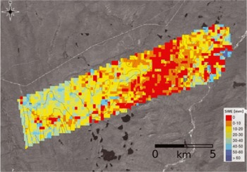
Fig. 4. Map of SWE changes (color-coded) between the November 2007 and February 2008 Cold Land Processes Experiment-II (CLPXII) campaigns at the Kuparuk River Study Site, Alaska. Background: Landsat image with 10m elevation contour lines. Database for SWE retrieval: PolScat Ku-band VV and VH, TerraSAR-X VV and VH. Courtesy Helmut Rott.
Vegetation also poses a problem with SWE retrievals from radar. While short, sparse shrubs and grasses are not likely to have a major effect on radar backscatter from the snowpack, taller shrubs and trees will strongly attenuate the radar backscatter. Ground measurements and simulations involving subarctic coniferous forest show that when the radar footprint contains high biomass (>100 m3 ha-1) or high vegetation fraction (>25%), the radar backscatter is not particularly sensitive to SWE (Reference Magagi, Bernier and BouchardMagagi and others, 2002).
Other considerations that are important for radar data include geometric distortions in mountainous terrain, a repeat orbit time (24−35 days) that is long relative to the timescale of snowpack processes, and the inability to perform accurate model inversion for SWE when the snow is vertically inhomogeneous or when the snow is melting.
6. Melting Snow
Detecting the onset of snowmelt has applications to hydrology and climatology since it indicates the earliest possible date for snowmelt runoff. The presence of even a small amount of liquid water in a snowpack severely limits the utility of passive microwave data since wet snow has an emissivity comparable to that of snow-free land. Using a time-series approach, Reference Walker and GoodisonWalker and Goodison (1993) developed a wet snow indicator for passive microwave data over the prairie region of western Canada. Comparing successive overpasses in which snow ‘disappeared’ and ‘reappeared’ in the microwave images, they could detect winter melt events and discern areas of snow even when wet.
Experiments with spaceborne radars such as Seasat and ERS-1/-2 have shown that these instruments are capable of mapping areas of wet snow and of retrieving snow liquid water content. These C-band SAR instruments, while not effective for measuring dry snow, can be used to identify melt events because the penetration depths in wet snow are much less. Using a change detection algorithm, Reference Nagler and RottNagler and Rott (2000) found that C-band SAR was an effective tool for mapping melting snow. Reference PulliainenPulliainen and others (2004) demonstrated the potential of using C-band SAR to map liquid water content in the boreal forest biome.
More recently, scatterometry has shown promise for mapping the melt state of snow. Reference Nghiem and TsaiNghiem and Tsai (2001) used Ku-band data from the NASA scatterometer (NSCAT) to map the melting snow conditions responsible for the April 1997 floods in the US northern plains and Canadian prairie region. Later, Reference Wang, Derksen and BrownWang and others (2008) used Ku-band data from QuikSCAT to identify areas of melting snow over the Arctic and found very good agreement with melt-onset and melt-end (snow disappearance) dates except in the boreal forest where vegetation causes a decreased sensitivity of backscatter to snowpack properties.
Hyperspectral data from the Airborne Visible/Infrared Imaging Spectrometer (AVIRIS) have been used to simultaneously retrieve snow grain size and liquid water content at a location in the California Sierra Nevada (Reference Green, Dozier, Roberts and PainterGreen and others, 2002; Reference Dozier, Green, Nolin and PainterDozier and others, 2009). A radiative transfer model is used to compute snow grain size (using the method of Reference Nolin and DozierNolin and Dozier, 2000), and then a second application of a radiative transfer model is used to find the best-fit estimate of liquid water content.
7. Snow Depth
Snow depth is a relevant measurement because of its relationship to snow water equivalent. Seasonal changes in snow depth can be related to changes in snow water equivalent if the density can be modeled or measured. At the regional-to-hemispheric scale, snow depth is controlled by climate processes (Reference Sturm, Holmgren and ListonSturm and others, 1995). At the watershed scale, spatial variations of snow depth often indicate wind redeposition, a process that is typically included in snow models but has not been widely validated.
Reference Nghiem and TsaiNghiem and Tsai (2001) used a global dataset of spaceborne Ku-band scatterometer data to evaluate their potential for mapping snow properties. They found that backscatter is sensitive to the seasonal evolution of snow depth in various snow climates.
Airborne and terrestrial lidar instruments have demonstrated abilities to measure snow depth. Lidar does not measure depth directly. Lidar data are acquired over an area prior to snowfall, and the lidar returns are converted into a bare earth model of the snow-free land surface. The procedure is repeated later in the season when snow is present to create a map of the snow surface. The height difference between the bare earth and snow surface is inferred to represent snow depth.
Airborne lidar has been successful in mapping snow depth at the watershed scale (Reference Hopkinson, Sitar, Chasmer and TreltzHopkinson and others, 2004; Reference Deems, Painter and GleasonDeems and Painter, 2006; Reference Deems, Painter and GleasonDeems and others 2006). Over non-mountainous terrain, airborne lidar systems exhibit ˜15−20cm vertical accuracy. However, flight limitations over mountain regions often require that the airborne lidar fly at a fixed altitude, which results in varying footprint size and slightly lower vertical and horizontal accuracies. Moreover, ground control points for orthorectification require ground-based kinematic GPS, which can be difficult in rugged environments during winter months. Horizontal accuracy is a critical factor for lidar measurements of snow depth in steep terrain because location errors along steep slopes will translate into large errors in snow depth.
Technological advances in terrestrial laser scanning (TLS) hold the promise of watershed-scale snow depth surveys with horizontal spatial resolution of ˜5 m and vertical errors less than 10 cm (Reference Prokop, Schirmer, Rub, Lehning and StockerProkop and others, 2008; Grunewald and others, 2010). Permanent reflectors can be mounted throughout the survey area to provide control points for the TLS data. Figure 5 shows TLS retrievals of snow depth for a small catchment in the Swiss Alps. The advantages of this ground-based remote-sensing technique are that it costs less than airborne lidar mapping and has excellent repeat accuracy with centimeter-scale precision. Of course as with any remote-sensing technique, it is not without limitations. TLS instruments work best for distances less than 1.5 km. Obstructions of the field of view by vegetation and topography also can be a problem, though with multiple survey points these can be minimized.

Fig. 5. Snow depth (HS) computed as the difference between snow-free and snow-covered conditions using a TLS in the Wannengrat catchment, Switzerland. Courtesy Michael Lehning and Thomas Grünewald
Conclusions
The past decade has seen major advances in remote-sensing instrumentation as well as modeling and analysis techniques. Collaborations within and external to the community of snow scientists have helped identify knowledge gaps, leading to major field campaigns aimed at finding innovative and tractable methods for filling these gaps. For the first time, groups of snow scientists have been at the forefront in proposing new satellite missions that are specific to seasonal snow. Still, much remains to be done.
Exploiting multi-sensor approaches is appealing since instrument limitations (e.g. temporal resolution, cloud problems) can be minimized while simultaneously maximizing synergies (e.g. multiple observations to increase temporal resolution, combining independent information to improve snow property retrievals). New work by Reference FosterFoster and others (2008) that combines MODIS (visible/near-infrared), AMSR-E (passive microwave) and QuikSCAT (scatterometer) is showing some success, but full validation and error assessment remains to be done.
There currently is no mathematically rigorous theory or physically based approaches that address the problem of scale in remote sensing. Reference Tedesco, Kim, Gasiewski, Klein and StankovTedesco and others (2005, Reference Tedesco2006) rightly note that ‘Perhaps the biggest issue regarding the use of such satellite measurements involves how to relate measurements made at spatial scales as small as the plot scale to observations from sensors with footprints that may be up to 25 km × 25 km’. Using linear stochastic analysis, Reference BlöschlBlöschl (1999) showed that the ratio of measurement scale to the process scale controls the degree to which scale influences interpretations of data and it can be especially difficult to assess patterns when the variability spans several orders of magnitude.
Addressing the problematic effects of forest canopy also remains a major challenge for virtually all types of remote sensing. In particular, information on the canopy structure (especially height and density) is needed to develop canopy adjustments for snow-cover measurements from multispectral, passive microwave, and radar instruments. Multiangular and lidar observations have the capability to provide this canopy structure information. Lastly, developing tractable approaches for data assimilation into hydrologic and climatologic models is a computational challenge that will require innovative approaches to gap filling, spatial scaling and a thorough understanding of errors associated with remotely sensed snow properties.
Acknowledgements
I am most grateful to T. Painter, J. Dozier, H. Rott, M. Lehning and T. Grunewald for contributing figures to this paper. Comments from the reviewers were much appreciated and significantly improved the manuscript.


