


1. Introduction
In optimal design one aims to find an optimal shape which minimizes a cost functional. The optimal shape is a subset  $E$ of a bounded, open set $\Omega \subset \mathbb {R}^N$ which is described by its characteristic function $\chi : \Omega \to \{0,1\}$, $E = \{\chi = 1\}$, and, in the linear elasticity framework, the cost functional is usually a quadratic energy, so we are lead to the problem

where  $W_0$ and $W_1$ are two elastic densities, with $W_0 \geq W_1$, and ${\mathcal {E}} u$ denotes the symmetrized gradient of the displacement $u$. We refer to the seminal papers [Reference Allaire and Lods1, Reference Kohn and Strang35–Reference Kohn and Strang37, Reference Murat and Tartar43], among a wide literature (see, for instance, the recent contributions [Reference Babadjian, Iurlano and Rindler7, Reference Babadjian, Iurlano and Rindler8]).
However, as soon as plasticity comes into play, the observed stress–strain relation is no longer linear and, due to the linear growth of the stored elastic energy and to the lack of reflexivity of the space  $L^1$, a suitable functional space is necessary to account for fields $u$ whose strains are measures. The space of special fields with bounded deformation, $BD(\Omega )$, was first proposed in [Reference Kohn and Strang36, Reference Kohn and Strang37, Reference Suquet47–Reference Suquet50] and starting from these pioneering papers a vast literature developed.
Indeed, already in the case where  $\chi \equiv \chi _\Omega$, the search for equilibria in the context of perfect plasticity leads naturally to the study of lower semicontinuity properties, and eventually relaxation, for energies of the type

where  $f$ is the volume energy density. As mentioned above, $u$ belongs to the space $BD(\Omega )$ of functions of bounded deformation composed of integrable vector-valued functions for which all components $E_{ij}$, $i,j = 1,\ldots,N$, of the deformation tensor $Eu := {(Du + Du^T)}/{2}$ are bounded Radon measures and ${\mathcal {E}} u$ stands for the absolutely continuous part, with respect to the Lebesgue measure, of the symmetrized distributional derivative $Eu$.
$Eu$.
Lower semicontinuity for (1.2) was established in [Reference Bellettini, Coscia and Dal Maso16] under convexity assumptions on  $f$ and in [Reference Ebobisse27] for symmetric quasiconvex integrands, under linear growth conditions and for $u \in LD(\Omega )$, the subspace of $BD(\Omega )$ comprised of functions for which the singular part $E^su$ of the measure $Eu$ vanishes. For a symmetric quasiconvex density $f$ with an explicit dependence on the position in the body and satisfying superlinear growth assumptions, lower semicontinuity properties were established in [Reference Ebobisse28] for $u \in SBD(\Omega )$.
In the case where the energy density takes the form  $\|{\mathcal {E}} u\|^2$ or $\|{\mathcal {E}}^D u\|^2 + (\text {div}\, u)^2$ (where $A^D$ stands for the deviator of the $N \times N$ matrix $A$ given by $A^D := A - ({1}/{N})\text {tr} (A)I$), and the total energy also includes a surface term, a first relaxation result was proved in [Reference Braides, Defranceschi and Vitali18]. We also refer to [Reference Kosiba and Rindler39] for the relaxation in the case where there is no surface energy and to [Reference Jesenko and Schmidt33, Reference Matias, Morandotti and Santos40, Reference Mora42] for related models concerning evolutions and homogenization, among a wider list of contributions.
For general energy densities  $f$, Barroso, Fonseca and Toader [Reference Barroso, Fonseca and Toader12] studied the relaxation of (1.2) for $u \in SBD(\Omega )$ under linear growth conditions but placing no convexity assumptions on $f$. They showed that the relaxed functional admits an integral representation where a surface energy term arises naturally. The global method for relaxation due to Bouchitté, Fonseca and Mascarenhas [Reference Bouchitté, Fonseca and Mascarenhas17] was used to characterize the density of this term, whereas the identification of the relaxed bulk energy term relied on the blow-up method [Reference Fonseca and Müller31] together with a Poincaré-type inequality.
Ebobisse and Toader [Reference Ebobisse and Toader29] obtained an integral representation result for general local functionals defined in  $SBD(\Omega )$ which are lower semicontinuous with respect to the $L^1$ topology and satisfy linear growth and coercivity conditions. The functionals under consideration are restrictions of Radon measures and are assumed to be invariant with respect to rigid motions. Their work was extended to the space $SBD^p(\Omega )$, $p > 1$, which arises in connection with the study of fracture and damage models, by Conti, Focardi and Iurlano [Reference Conti, Focardi and Iurlano24] in the two-dimensional setting. A crucial and novel ingredient of their proof is the construction of a $W^{1,p}$ approximation of an $SBD^p$ function $u$ using finite-elements on a countable mesh which is chosen according to $u$ (recall that $SBD^p$ denotes the space of fields with bounded deformation such that the symmetrized gradient is the sum of an $L^p$ field and a measure supported on a set of finite $\mathcal {H}^{N-1}$ measure).
The analysis of an integral representation for a variational functional satisfying lower semicontinuity, linear growth conditions and the usual measure theoretical properties, was extended to the full space  $BD(\Omega )$ by Caroccia, Focardi and Van Goethem [Reference Caroccia, Focardi and Van Goethem23]. In this work, the invariance of the studied functional with respect to rigid motions, required in [Reference Ebobisse and Toader29], is replaced by a weaker condition stating continuity with respect to infinitesimal rigid motions. Their result relies, as in papers mentioned above, on the global method for relaxation, as well as on the characterization of the Cantor part of the measure $Eu$, due to De Philippis and Rindler [Reference De Philippis and Rindler25], which extends to the $BD$ case the result of Alberti's rank-one theorem in $BV$.
$BV$.
In the study of the minimization problem (1.1) one usually prescribes the volume fraction of the optimal shape, leading to a constraint of the form  $\displaystyle \frac {1}{{\mathcal {L}}^N(\Omega )}\int _\Omega \chi (x)\,{\rm d}x= \theta,\;\theta \in (0,1)$. It is sometimes convenient to replace this constraint by inserting, instead, a Lagrange multiplier in the modelling functional which, in the optimal design context, becomes

Despite the fact that we have compactness for  $u$ in $BD(\Omega )$ for functionals of the form (1.3), it is well known that the problem of minimizing (1.3) with respect to $(\chi,u)$, adding suitable forces and/or boundary conditions, is ill-posed, in the sense that minimizing sequences $\chi _n \in L^\infty (\Omega ;\{0,1\})$ tend to highly oscillate and develop microstructure, so that in the limit we may no longer obtain a characteristic function. To avoid this phenomenon, as in [Reference Ambrosio and Buttazzo2, Reference Kohn and Lin34], we add a perimeter penalization along the interface between the two zones $\{\chi = 0\}$ and $\{\chi = 1\}$ (see [Reference Carita and Zappale21] for the analogous analysis performed in $BV$, and [Reference Barroso and Zappale14, Reference Barroso and Zappale15, Reference Carita and Zappale20] for the Sobolev settings, also in the presence of a gap in the growth exponents).
Thus, with an abuse of notation (i.e. denoting  $W_1+ k$, in (1.3), still by $W_1$), our aim in this paper is to study the energy functional given by

where  $u \in BD(\Omega )$, $\chi \in BV(\Omega ;\{0,1\})$ and the densities $W_i$, $i = 0,1$, are continuous functions satisfying the following linear growth conditions from above and below:

We point out that no convexity assumptions are placed on  $W_i$, $i = 0,1$.
To simplify the notation, in the sequel, we let  $f: \{0,1\} \times \mathbb {R}^{N \times N}_s \to [0,+\infty )$ be defined as

and for a fixed  $q \in \{0,1\}$, we recall that the recession function of $f$, in its second argument, is given by
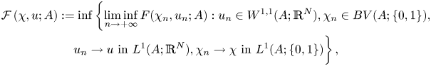
Since we place no convexity assumptions on  $W_i$, we consider the relaxed localized functionals arising from the energy (1.4), defined, for an open subset $A \subset \Omega$, by
and
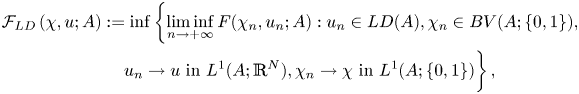
where  $LD(\Omega ):=\{u \in BD(\Omega ): E^s u=0\}$.
Due to the expression of (1.4), and to the fact that  $\chi _n \mathop {\rightharpoonup }\limits ^{\ast }\chi$ in $BV$ if and only if $\{\chi _n\}$ is uniformly bounded in $BV$ and $\chi _n \to \chi$ in $L^1$, it is equivalent to take $\chi _n \mathop {\rightharpoonup }\limits ^{\ast }\chi$ in $BV$ or $\chi _n \to \chi$ in $L^1$ in the definitions of the functionals (1.8) and (1.9), obtaining for each of them the same infimum regardless of the considered convergence.
As a simple consequence of the density of smooth functions in  $LD(\Omega )$ we show in remark 3.5 that, under the above growth conditions on $W_0, W_1$,

We prove in proposition 3.8 that  $\mathcal {F}\left (\chi,u;\cdot \right )$ is the restriction to the open subsets of $\Omega$ of a Radon measure, the main result of our paper concerns the characterization of this measure.
Theorem 1.1 Let  $f:\{0,1\} \times \mathbb {R}^{N \times N}_s\to [0, + \infty )$ be a continuous function as in (1.6), where $W_0$ and $W_1$ satisfy (1.5), and consider $F:BV(\Omega ;\{0,1\})\times BD(\Omega )\times \mathcal {O}(\Omega )$ defined in (1.4). Then

where  $SQf$ is the symmetric quasiconvex envelope of $f$ and $(SQf)^{\infty }$ is its recession function $($cf. § 2.3 and (1.7), respectively $)$. The relaxed surface energy density is given by

where  $Q_{\nu }(x_0,{\varepsilon })$ stands for an open cube with centre $x_0$, sidelength ${\varepsilon }$ and two of its faces parallel to the unit vector $\nu$,

for any  $V$ open subset of $\Omega$ with Lipschitz boundary, and, for $(a,b,c,d,\nu ) \in \{0,1\} \times \{0,1\} \times \mathbb {R}^{N} \times \mathbb {R}^{N} \times S^{N-1},$ the functions $\chi _{a,b,\nu }$ and $u_{c,d,\nu }$ are defined as

For the notation regarding the jump sets  $J_\chi$, $J_u$ and the corresponding vectors $\chi ^+(x)$, $\chi ^-(x)$, $\nu _\chi (x)$, $u^+(x)$, $u^-(x)$ and $\nu _u(x)$ we refer to § 2.1, 2.2 and 4.3.
The above expression for the relaxed surface energy density arises as an application of the global method for relaxation [Reference Bouchitté, Fonseca and Mascarenhas17]. However, as we will see in § 4.3, in the case where  $f$ satisfies the additional hypothesis (3.9), this density can be described more explicitly, leading to an integral representation for (1.8), in the $BD$ setting, entirely similar to the one in $BV$, obtained in [Reference Carita and Zappale21], when $W_0$ and $W_1$ depend on the whole gradient $\nabla u$. Indeed, under this assumption, we show that

where

and, for  $(a,b,c,d,\nu ) \in \{0,1\} \times \{0,1\} \times \mathbb {R}^{N} \times \mathbb {R}^{N} \times S^{N-1},$ the set of admissible functions is
 $\left \{\nu _{1},\nu _{2},\dots,\nu _{N-1},\nu \right \}$ is an orthonormal basis of $\mathbb {R}^{N}$ and $S_\nu$ is the strip given by

As an application of the result of Caroccia, Focardi and Van Goethem, obtained in the abstract variational functional setting in [Reference Caroccia, Focardi and Van Goethem23], the authors proved an integral representation for the relaxed functional, defined in  $BD(\Omega ) \times \mathcal {O}(\Omega )$,

where

and the density  $f_0$ satisfies linear growth conditions from above and below

as well as a continuity condition with respect to  $(x,u)$. This generalizes to the full space $BD(\Omega )$, and to the case of densities $f_0$ depending explicitly on $(x,u)$, the results obtained in [Reference Barroso, Fonseca and Toader12]. We will make use of their work in § 4.2 to prove both lower and upper bounds for the density of the Cantor part of the measure $\mathcal {F}(\chi,u;\cdot )$, by means of an argument based on Chacon's biting lemma which allows us to fix $\chi$ at an appropriately chosen point $x_0$, as in [Reference Matias, Morandotti and Zappale41].
The contents of this paper are organized as follows. In § 2 we fix our notation and provide some results pertaining to  $BV$ and $BD$ functions and notions of quasiconvexity which will be used in the sequel. Section 3 contains some auxiliary results which are needed to prove our main theorem. In particular, in proposition 3.8 we show that $\mathcal {F}(\chi,u;\cdot )$ is the restriction to the open subsets of $\Omega$ of a Radon measure $\mu$. Section 4 is dedicated to the proof of our main theorem, which characterizes this measure. In each of § 4.1, 4.2 and 4.3 we prove lower and upper bounds of the densities of $\mu$ with respect to the bulk and Cantor parts of $Eu$, as well as with respect to a surface measure which is concentrated on the union of the jump sets of $\chi$ and $u$.
$u$.
The fact that our functionals have an explicit dependence on the  $\chi$ field prevented us from applying existing results (such as [Reference Arroyo-Rabasa, De Philippis and Rindler5, Reference Breit, Diening and Gmeineder19]) directly and required us to obtain direct proofs.
2. Preliminaries
In this section we fix notations and quote some definitions and results that will be used in the sequel.
Throughout the text  $\Omega \subset \mathbb {R}^{N}$ will denote an open, bounded set with Lipschitz boundary.
We will use the following notations:
• ${\mathcal {B}}(\Omega )$, ${\mathcal {O}}(\Omega )$ and ${\mathcal {O}}_{\infty }(\Omega )$ represent the families of all Borel, open and open subsets of $\Omega$ with Lipschitz boundary, respectively;
•
$\mathcal {M} (\Omega )$ is the set of finite Radon measures on $\Omega$;•
$\left |\mu \right |$ stands for the total variation of a measure $\mu \in \mathcal {M} (\Omega )$;•
$\mathcal {L}^{N}$ and $\mathcal {H}^{N-1}$ stand for the $N$-dimensional Lebesgue measure and the $\left (N-1\right )$-dimensional Hausdorff measure in $\mathbb {R}^N$, respectively;• the symbol
${\rm d} x$ will also be used to denote integration with respect to $\mathcal {L}^{N}$;• the set of symmetric
$N \times N$ matrices is denoted by $\mathbb{R}_s^{N\times N}$;• given two vectors
$a, b \in {\mathbb {R}}^N$, $a \odot b$ is the symmetric $N \times N$ matrix defined by $a \odot b : = \dfrac {a \otimes b + b \otimes a}{2}$, where $\otimes$ indicates tensor product;•
$B(x, {\varepsilon })$ is the open ball in ${\mathbb {R}}^N$ with centre $x$ and radius ${\varepsilon }$, $Q(x,{\varepsilon })$ is the open cube in ${\mathbb {R}}^N$ with two of its faces parallel to the unit vector $e_N$, centre $x$ and sidelength ${\varepsilon }$, whereas $Q_{\nu }(x,{\varepsilon })$ stands for a cube with two of its faces parallel to the unit vector $\nu$; when $x=0$ and ${\varepsilon } = 1$, $\nu =e_N$ we simply write $B$ and $Q$;•
$S^{N-1} := \partial B$ is the unit sphere in ${\mathbb {R}}^N$;•
$C_c^{\infty }(\Omega ; {\mathbb {R}}^N)$ and $C_{\rm per}^{\infty }(Q; {\mathbb {R}}^N)$ are the spaces of ${\mathbb {R}}^N$-valued smooth functions with compact support in $\Omega$ and smooth and $Q$-periodic functions from $Q$ to ${\mathbb {R}}^N$, respectively;• by
$\displaystyle \lim _{\delta, n}$ we mean $\displaystyle \lim _{\delta \to 0^+} \lim _{n\to +\infty }$, $\displaystyle \lim _{k, n}$ means $\displaystyle \lim _{k \to +\infty } \lim _{n\to +\infty }$;•
$C$ represents a generic positive constant that may change from line to line.


2.1 BV functions and sets of finite perimeter
In the following we give some preliminary notions regarding functions of bounded variation and sets of finite perimeter. For a detailed treatment we refer to [Reference Ambrosio, Fusco and Pallara4].
Given  $u \in L^1(\Omega ; {\mathbb {R}}^d)$ we let $\Omega _u$ be the set of Lebesgue points of $u$, i.e. $x\in \Omega _u$ if there exists $\widetilde u(x)\in {\mathbb {R}}^d$ such that
 $\widetilde u(x)$ is called the approximate limit of $u$ at $x$. The Lebesgue discontinuity set $S_u$ of $u$ is defined as $S_u := \Omega {\setminus} \Omega _u$. It is known that ${\mathcal {L}}^{N}(S_u) = 0$ and the function $x \in \Omega \mapsto \widetilde u(x)$, which coincides with $u$
$u$  ${\mathcal {L}} ^N$-a.e. in $\Omega _u$, is called the Lebesgue representative of $u$.
$u$.
The jump set of the function  $u$, denoted by $J_u$, is the set of points $x\in \Omega {\setminus} \Omega _u$ for which there exist $a,\,b\in {\mathbb {R}}^d$ and a unit vector $\nu \in S^{N-1}$, normal to $J_u$ at $x$, such that $a\neq b$ and

The triple  $(a,b,\nu )$ is uniquely determined by the conditions above, up to a permutation of $(a,b)$ and a change of sign of $\nu$, and is denoted by $(u^+ (x),u^- (x),\nu _u (x)).$ The jump of $u$ at $x$ is defined by $[u](x) : = u^+(x) - u^-(x).$
We recall that a function  $u\in L^{1}(\Omega ;{\mathbb {R}}^{d})$ is said to be of bounded variation, and we write $u\in BV(\Omega ;{\mathbb {R}}^{d})$, if all its first-order distributional derivatives $D_{j}u_{i}$ belong to $\mathcal {M}(\Omega )$ for $1\leq i\leq d$ and $1\leq j\leq N$.
The matrix-valued measure whose entries are  $D_{j}u_{i}$ is denoted by $Du$ and $|Du|$ stands for its total variation. The space $BV(\Omega ; {\mathbb {R}}^d)$ is a Banach space when endowed with the norm

and we observe that if  $u\in BV(\Omega ;\mathbb {R}^{d})$ then $u\mapsto |Du|(\Omega )$ is lower semicontinuous in $BV(\Omega ;\mathbb {R}^{d})$ with respect to the $L_{\mathrm {loc}}^{1}(\Omega ;\mathbb {R}^{d})$ topology.
By the Lebesgue decomposition theorem,  $Du$ can be split into the sum of two mutually singular measures $D^{a}u$ and $D^{s}u$, the absolutely continuous part and the singular part, respectively, of $Du$ with respect to the Lebesgue measure $\mathcal {L}^N$. By $\nabla u$ we denote the Radon–Nikodým derivative of $D^{a}u$ with respect to $\mathcal {L}^N$, so that we can write

If  $u \in BV(\Omega )$ it is well known that $S_u$ is countably $(N-1)$-rectifiable, see [Reference Ambrosio, Fusco and Pallara4], and the following decomposition holds

where  $D^cu$ is the Cantor part of the measure $Du$.
$Du$.
If  $\Omega$ is an open and bounded set with Lipschitz boundary then the outer unit normal to $\partial \Omega$ (denoted by $\nu$) exists ${\mathcal {H}}^{N-1}$-a.e. and the trace for functions in $BV(\Omega ;{\mathbb {R}}^d)$ is defined.
Theorem 2.1 (Approximate differentiability)
If  $u \in BV(\Omega ; {\mathbb {R}}^d),$ then for $\mathcal {L}^N$-a.e. $x \in \Omega$

Definition 2.2 Let  $E$ be an $\mathcal {L}^{N}$-measurable subset of $\mathbb {R}^{N}$. For any open set $\Omega \subset \mathbb {R}^{N}$ the perimeter of $E$ in $\Omega$, denoted by $P(E;\Omega )$, is given by

We say that  $E$ is a set of finite perimeter in $\Omega$ if $P(E;\Omega ) <+ \infty.$
Recalling that if  $\mathcal {L}^{N}(E \cap \Omega )$ is finite, then $\chi _{E} \in L^{1}(\Omega )$, by [Reference Ambrosio, Fusco and Pallara4, proposition 3.6], it follows that $E$ has finite perimeter in $\Omega$ if and only if $\chi _{E} \in BV(\Omega )$ and $P(E;\Omega )$ coincides with $|D\chi _{E}|(\Omega )$, the total variation in $\Omega$ of the distributional derivative of $\chi _{E}$. Moreover, a generalized Gauss–Green formula holds:

where  $D\chi _{E}=\nu _{E}|D\chi _{E}|$ is the polar decomposition of $D\chi _{E}$.
The following approximation result can be found in [Reference Baldo9].
Lemma 2.3 Let  $E$ be a set of finite perimeter in $\Omega$. Then, there exists a sequence of polyhedra $E_n$, with characteristic functions $\chi _n$, such that $\chi _n\to \chi$ in $L^1(\Omega ;\{0,1\})$ and $P (E_n;\Omega )\to P(E;\Omega )$.
2.2 BD and LD functions
We now recall some facts about functions of bounded deformation. More details can be found in [Reference Ambrosio, Coscia and Dal Maso3, Reference Barroso, Fonseca and Toader12, Reference Bellettini, Coscia and Dal Maso16, Reference Temam51, Reference Temam and Strang52].
A function  $u\in L^{1}(\Omega ;{\mathbb {R}}^{N})$ is said to be of bounded deformation, and we write $u\in BD(\Omega )$, if the symmetric part of its distributional derivative $Du$,
$Du$,  $Eu: = {(Du + Du^T)}/{2},$ is a matrix-valued bounded Radon measure. The space $BD(\Omega )$ is a Banach space when endowed with the norm

We denote by  $LD(\Omega )$ the subspace of $BD(\Omega )$ comprised of functions $u$ such that $Eu \in L^1(\Omega ;{\mathbb {R}}^{N\times N}_s)$, a counterexample due to [Reference Ornstein44] shows that $W^{1,1}(\Omega ;\mathbb {R}^N) \subsetneq LD(\Omega )$.
The intermediate topology in the space  $BD(\Omega )$ is the one determined by the distance

Hence, a sequence  $\{u_n\} \subset BD(\Omega )$ converges to a function $u \in BD(\Omega )$ with respect to this topology, written $u_n \stackrel {i}{\to }u$, if and only if, $u_n \to u$ in $L^1(\Omega ;{\mathbb {R}}^N)$, $Eu_n \stackrel {*}{\rightharpoonup } Eu$ in the sense of measures and $|Eu_n|(\Omega ) \to |Eu|(\Omega )$.
Recall that if  $u_n \to u$ in $L^1(\Omega ;{\mathbb {R}}^N)$ and there exists $C > 0$ such that $|Eu_n|(\Omega ) \leq C, \forall n \in {\mathbb {N}}$, then $u \in BD(\Omega )$ and

By the Lebesgue decomposition theorem,  $Eu$ can be split into the sum of two mutually singular measures $E^{a}u$ and $E^{s}u$, the absolutely continuous part and the singular part, respectively, of $Eu$ with respect to the Lebesgue measure $\mathcal {L}^N$. The Radon–Nikodým derivative of $E^{a}u$ with respect to $\mathcal {L}^N$, is denoted by ${\mathcal {E}} u$ so we have

With these notations we may write

and (cf. [Reference Temam51])  $LD(\Omega )$ is a Banach space when endowed with the norm

If  $\Omega$ is a bounded, open subset of ${\mathbb {R}}^N$ with Lipschitz boundary $\Gamma$, then there exists a linear, surjective and continuous, both with respect to the norm and to the intermediate topologies, trace operator

such that tr  $u = u$ if $u \in BD(\Omega ) \cap C(\overline {\Omega };{\mathbb {R}}^N)$. Furthermore, the following Gauss–Green formula holds

for every  $\varphi \in C^1(\overline {\Omega })$ (cf. [Reference Ambrosio, Coscia and Dal Maso3, Reference Temam51]).
The following lemma is proved in [Reference Barroso, Fonseca and Toader12].
Lemma 2.4 Let  $u \in BD(\Omega )$ and let $\rho \in C_0^{\infty }({\mathbb {R}}^N)$ be a non-negative function such that ${\rm supp}(\rho ) \subset \subset B(0,1)$, $\rho (-x) = \rho (x)$ for every $x \in {\mathbb {R}}^N$ and $\int _{{\mathbb {R}}^N}\rho (x)\,{\rm d}x = 1$. For any $n \in {\mathbb {N}}$ set $\rho _n(x) : = n^N\rho (nx)$ and

Then  $u_n \in C^{\infty }\left (\left \{y \in \Omega : {\rm dist}(y,\partial \Omega ) > \frac {1}{n}\right \};{\mathbb {R}}^N\right )$ and
(i) for any non-negative Borel function
$h : \Omega \to {\mathbb {R}}$
\[ \int_{B(x_0,\varepsilon)}h(x) |{\mathcal{E}} u_n(x)|\,{\rm d}x \leq\int_{B(x_0,\varepsilon+ {1}/{n})}(h*\rho_n)(x)\,{\rm d}|E u|(x), \]whenever${\varepsilon } + \frac {1}{n} < {\rm dist}(x_0,\partial \Omega );$(ii) for any positively homogeneous of degree one, convex function
$\theta : {\mathbb {R}}^{N\times N}_{\rm sym} \to [0,+\infty [$ and any ${\varepsilon } \in \, ]0,{\rm dist}(x_0,\partial \Omega )[$ such that $|E u|(\partial B(x_0,{\varepsilon })) = 0$,
\[ \lim_{n\rightarrow +\infty}\int_{B(x_0,\varepsilon)} \theta({\mathcal{E}} u_n(x))\,{\rm d}x =\int_{B(x_0,\varepsilon)}\theta\left(\frac{{\rm d}Eu}{{\rm d}|Eu|}\right)\,{\rm d}|Eu|, \](iii)
$\lim _{n \to + \infty }u_n(x) = \widetilde u(x)$ and $\lim _{n \to + \infty }(|u_n -u| * \rho _n)(x) = 0$ for every $x \in \Omega {\setminus} S_u$, whenever $u \in L^{\infty }(\Omega ;{\mathbb {R}}^N)$.


The following result, proved in [Reference Temam51], see also [Reference Barroso, Fonseca and Toader12, theorem 2.6], shows that it is possible to approximate any  $BD(\Omega )$ function $u$ by a sequence of smooth functions which preserve the trace of $u$.
$u$.
Theorem 2.5 Let  $\Omega$ be a bounded, connected, open set with Lipschitz boundary. For every $u \in BD(\Omega )$, there exists a sequence of smooth functions $\{u_n\} \subset C^{\infty }(\Omega ;{\mathbb {R}}^N) \cap W^{1,1}(\Omega ;{\mathbb {R}}^N)$ such that $u_n \stackrel {i}{\to }u$ and tr $u_n =$ tr $u$. If, in addition, $u \in LD(\Omega )$, then ${\mathcal {E}} u_n \to {\mathcal {E}} u$ in $L^1(\Omega ;\mathbb{R}_s^{N\times N}).$
It is also shown in [Reference Temam51] that if  $\Omega$ is an open, bounded subset of ${\mathbb {R}}^N$, with Lipschitz boundary, then $BD(\Omega )$ is compactly embedded in $L^q(\Omega ;{\mathbb {R}}^N)$, for every $1 \leq q < {N}/{(N-1)}.$ In particular, the following result holds.
Theorem 2.6 Let  $\Omega$ be an open, bounded subset of $\mathbb {R}^N$, with Lipschitz boundary and let $1\leq q <{N}/{(N-1)}$. If $\{u_n\}$ is bounded in $BD(\Omega )$, then there exist $u \in BD(\Omega )$ and a subsequence $\{ u_{n_k}\}$ of $\{u_n\}$ such that $u_{n_k}\to u$ in $L^q (\Omega ;\mathbb {R}^N)$.
If  $u \in BD(\Omega )$ then $J_u$ is countably $(N-1)$-rectifiable, see [Reference Ambrosio, Coscia and Dal Maso3], and the following decomposition holds

where  $[u] = u^+ - u^-$, $u^{\pm }$ are the traces of $u$ on the sides of $J_u$ determined by the unit normal $\nu _u$ to $J_u$ and $E^cu$ is the Cantor part of the measure $Eu$ which vanishes on Borel sets $B$ with $\mathcal {H}^{N-1}(B) < + \infty.$
We end this subsection by pointing out that the equivalent of (2.1), with  ${\mathcal {E}} u(x)$ replacing $\nabla u(x)$, is false (see [Reference Ambrosio, Coscia and Dal Maso3]). However the following result holds (cf. [Reference Ambrosio, Coscia and Dal Maso3, theorem 4.3] and [Reference Ebobisse28, theorem 2.5]).
Theorem 2.7 (Approximate symmetric differentiability)
If  $u \in BD(\Omega ),$ then, for $\mathcal {L}^N$-a.e. $x \in \Omega$, there exists an $N\times N$ matrix $\nabla u(x)$ such that


for  $\mathcal {L}^N$-a.e. $x \in \Omega$. Furthermore

with  $C(N,\Omega )>0$ depending only on $N$ and $\Omega$.
From (2.5) and (2.6) it follows that  ${\mathcal {E}} u={(\nabla u+\nabla u^T)}/{2}$.
We denote by  $\mathcal {R}$ the kernel of the linear operator $E$ consisting of the class of rigid motions in $\mathbb {R}^N$, i.e. affine maps of the form $Mx + b$ where $M$ is a skew-symmetric $N \times N$ matrix and $b\in \mathbb {R}^N$. $\mathcal {R}$ is therefore closed and finite-dimensional so it is possible to define the orthogonal projection $P : BD(\Omega )\to \mathcal {R}$. This operator belongs to the class considered in the following Poincaré–Friedrichs type inequality for $BD$ functions (see [Reference Ambrosio, Coscia and Dal Maso3, Reference Kohn38, Reference Temam51]).
Theorem 2.8 Let  $\Omega$ be a bounded, connected, open subset of $\mathbb {R}^N$, with Lipschitz boundary, and let $R : BD(\Omega )\to \mathcal {R}$ be a continuous linear map which leaves the elements of $\mathcal {R}$ fixed. Then there exists a constant $C(\Omega, R)$ such that

2.3 Notions of quasiconvexity
Definition 2.9 ([Reference Barroso, Fonseca and Toader12], definition 3.1)
A Borel measurable function  $f:\mathbb {R}^{N\times N}_s\to \mathbb {R}$ is said to be symmetric quasiconvex if

for every  $\xi \in \mathbb {R}^{N\times N}_s$ and for every $\varphi \in C^{\infty }_{\rm per}(Q;\mathbb {R}^N)$.
Remark 2.10 The above property (2.7) is independent of the size, orientation and centre of the cube over which the integration is performed. Also, if  $f$ is upper semicontinuous and locally bounded from above, using Fatou's lemma and the density of smooth functions in $LD(Q)$, it follows that in (2.7) $C^{\infty }_{\rm per}(Q;\mathbb {R}^N)$ may be replaced by $LD_{\rm per}(Q).$
Given  $f:\mathbb {R}^{N\times N}_s\to \mathbb {R}$, the symmetric quasiconvex envelope of $f$,
$f$,  $SQf$, is defined by

It is possible to show that  $SQf$ is the greatest symmetric quasiconvex function that is less than or equal to $f$. Moreover, definition (2.8) is independent of the domain, i.e.

whenever  $D \subset {\mathbb {R}}^N$ is an open, bounded set with ${\mathcal {L}} ^N(\partial D) = 0$.
In [Reference Ebobisse27], a Borel measurable function  $f:\mathbb {R}^{N\times N}_s\to \mathbb {R}$ is said to be symmetric quasiconvex if and only if

and it is stated that  $f$ is symmetric quasiconvex if and only if $f\circ \pi$ is quasiconvex in the sense of Morrey, where $\pi$ is the projection of $\mathbb {R}^{N \times N}$ onto $\mathbb {R}^{N\times N}_{s}$.
Let us show that these two notions coincide. Observe first that, for any  $\varphi \in C^\infty _0(D;\mathbb {R}^N)$,

If  $f$ is upper semicontinuous and satisfies a growth condition from above as in (1.5), then $SQf$ in (2.9) is symmetric quasiconvex also in the sense of [Reference Ebobisse27]. Indeed, $SQf$ satisfies the same growth condition (1.5) and a density argument as in [Reference Ball and Murat10] shows that $SQf \circ \pi$ is $W^{1,1}$-quasiconvex, hence $W^{1,\infty }$-quasiconvex, i.e. $\varphi$ can be chosen in $W^{1,\infty }_0(D;\mathbb {R}^N)$. Thus,

for every  $\varphi \in W^{1,\infty }_0(D;\mathbb {R}^N)$. Therefore, denoting by $SQf_E$ the symmetric quasiconvexification

and by  $SQf$ the symmetric quasiconvexification defined through (2.9), trivially $SQf_E\leq SQf$ and by (2.12) we have equality.
Actually, under linear growth conditions and upper semicontinuity of  $f$, we may also conclude that

3. Auxiliary results
We recall that for  $u \in BD(\Omega )$ and $\chi \in BV(\Omega ;\{0,1\})$ the energy under consideration is

and our aim is to obtain an integral representation for the localized relaxed functionals, defined for  $A \in \mathcal {O}(\Omega )$, by


where the densities  $W_i$, $i = 0,1$, are continuous functions such that

and where, for purposes of notation, we let  $f: \{0,1\} \times \mathbb {R}^{N \times N}_s \to [0,+\infty )$ be defined as

It follows from the definition of the recession function (1.7) and from the growth conditions (3.4) that for every  $q \in \{0,1\}$ and every $\xi \in {\mathbb {R}}^{N \times N}_s$

It is an immediate consequence of (3.4) that

from which it follows that

The following additional hypothesis will be used to write the density of the jump term in the form given in (1.11)

for every  $q \in \{0,1\}$ and every $\xi \in {\mathbb {R}}^{N \times N}_s$. As pointed out in [Reference Fonseca and Müller32], this can be stated equivalently as

for every  $q \in \{0,1\}$ and every $\xi \in {\mathbb {R}}^{N \times N}_s$.
Under our assumed growth conditions (3.4), we observe that if  $f$ satisfies (3.9), or equivalently (3.10), then the same holds for its symmetric quasiconvex envelope $SQf$. To this end, we recall that, under the hypothesis (3.4), the recession function of a symmetric quasiconvex function is still symmetric quasiconvex (see [Reference Rindler46, remarks 8 and 9]) and we begin by stating the following results (cf. [Reference Carita and Zappale21, (iv) and (v) in remark 3.2] and [Reference Ribeiro and Zappale45, propositions 2.6 and 2.7] for the quasiconvex counterpart).
Proposition 3.1 Let  $f:\{0,1\} \times \mathbb {R}^{N \times N}_s\to [0, + \infty )$ be a continuous function as in (3.5) and satisfying (3.4) and (3.9). Let $f^\infty$ and $SQf$ be its recession function and its symmetric quasiconvex envelope, defined by (1.7) and (2.8), respectively. Then

Proposition 3.2 Let  $f:\{0,1\} \times \mathbb {R}^{N \times N}_s\to [0, + \infty )$ be a continuous function as in (3.5), satisfying (3.4) and (3.9). Then, there exist $\gamma \in [0,1)$ and $C>0$ such that

The growth conditions (3.4), as well as standard diagonalization arguments, allow us to prove the following properties of the functional  $\mathcal {F} (\chi,u;A)$ defined in (3.2).
Proposition 3.3 Let  $A \in \mathcal {O}(\Omega )$, $u \in BD(A)$, $\chi \in BV(A;\{0,1\})$ and $F(\chi,u;A)$ be given by (3.1). If $W_i$, $i = 0,1$, satisfy (3.4), then
(i) there exists
$C > 0$ such that
\[ C\left(|Eu|(A) + |D\chi|(A)\right) \leq \mathcal{F} (\chi,u;A) \leq C\left({\mathcal{L}}^N(A) + |Eu|(A) + |D\chi|(A)\right); \](ii)
$\mathcal {F} (\chi,u;A)$ is always attained, that is, there exist sequences $\{u_n\} \subset W^{1,1}(A;\mathbb {R}^{N})$ and $\{\chi _{n}\} \subset BV(A;\{0,1\})$ such that $u_{n}\to u$ in $L^{1}(A;\mathbb {R}^{N})$, $\chi _{n}\to \chi$ in $L^1(A;\{0,1\})$ and
\[ \mathcal{F}(\chi,u;A) = \lim_{n\rightarrow\infty}F(\chi_n,u_n;A); \](iii) if
$\{u_n\} \subset W^{1,1}(A;\mathbb {R}^{N})$ and $\{\chi _{n}\} \subset BV(A;\{0,1\})$ are such that $u_{n}\to u$ in $L^{1}(A;\mathbb {R}^{N})$ and $\chi _{n}\to \chi$ in $L^1(A;\{0,1\})$, then
\[ \mathcal{F}(\chi,u;A) \leq \liminf_{n\to +\infty}\mathcal{F}(\chi_n, u_n;A). \]


Proof.  $(i)$ The upper bound follows from the growth condition from above of $W_i$, $i=0,1$ and by fixing $\chi _n = \chi$ as a test sequence for $\mathcal {F} (\chi,u;A)$, whereas the lower bound is a consequence of the inequality from below in (3.4) and (2.3) and the lower semicontinuity of the total variation of Radon measures.
The conclusions in  $(ii)$ and $(iii)$ follow by standard diagonalization arguments.
Remark 3.4 Analogous conclusions also hold for the functional  $\mathcal {F}_{LD} (\chi,u;A)$.
Remark 3.5 Assuming that the continuous functions  $W_0$ and $W_1$ satisfy the growth hypothesis (3.4), it follows from the density of smooth functions in $LD(\Omega )$ and a diagonalization argument that

Proof. As  $W^{1,1}(A;\mathbb {R}^N) \subset LD(A)$, one inequality is trivial. In order to show the reverse one, let $\{u_n\} \subset LD(A)$, $\{\chi _n\} \subset BV(A;\left \{0,1\right \})$ be such that $u_{n}\to u$ in $L^{1}(A;\mathbb {R}^{N})$, $\chi _{n}\to \chi$ in $L^1(A;\{0,1\})$ and

By theorem 2.5, for each  $n \in {\mathbb {N}}$, let $v_{n,k} \in W^{1,1}(A;\mathbb {R}^N)$ be such that $v_{n,k} \to u_n$ in $L^{1}(A;\mathbb {R}^{N})$, as $k \to + \infty$, and ${\mathcal {E}} v_{n,k} \to {\mathcal {E}} u_n$ in $L^{1}(A;\mathbb {R}^{N\times N}_s)$, as $k \to + \infty$. By passing to a subsequence, if necessary, assume also that $\lim _{k\rightarrow +\infty }{\mathcal {E}} v_{n,k}(x) = {\mathcal {E}} u_n(x)$, for a.e. $x \in A$. By (3.4) and Fatou's lemma we obtain

so that

and likewise for the term involving  $(1 - \chi _n)W_0$. From the previous inequalities we conclude that

Since  $v_{n,k} \to u_n$ in $L^{1}(A;\mathbb {R}^{N})$, as $k \to + \infty$, and $u_{n}\to u$ in $L^{1}(A;\mathbb {R}^{N})$, by a diagonalization argument there exists a sequence $k_n \to + \infty$ such that $v_{n,k_n} \to u$ in $L^{1}(A;\mathbb {R}^{N})$ and

As  $\{\chi _n\}$, $\{v_{n,k_n}\}$ are admissible for $\mathcal {F}\left (\chi,u;A\right )$ it follows that

A straightforward adaptation of the proof of [Reference Barroso, Fonseca and Toader12, proposition 3.7] yields the following result which enables us to prove the nested subadditivity property of the functional  $\mathcal {F}\left (\chi,u;\cdot \right )$.
Proposition 3.6 Let  $A \in \mathcal {O} (\Omega )$ and assume that $W_0, W_1$ satisfy the growth condition (3.4). Let $\{\chi _n\} \subset BV(A;\{0,1\})$ and $\{u_n\}, \{v_n\} \subset BD(A;\mathbb {R}^N)$ be sequences satisfying $u_{n} - v_n \to 0$ in $L^{1}(A;\mathbb {R}^{N})$, $\sup _n |Eu_n|(A) < + \infty$, $|Ev_n| \mathop {\rightharpoonup }\limits ^{\ast } \mu$ and $|Ev_n| \to \mu (A)$. Then there exist subsequences $\{v_{n_k}\}$ of $\{v_n\}$, $\{\chi _{n_k}\}$ of $\{\chi _n\}$ and there exists a sequence $\{w_k\} \subset BD(A)$ such that $w_k = v_{n_k}$ near $\partial A$, $w_k - v_{n_k} \to 0$ in $L^{1}(A;\mathbb {R}^{N})$ and

It is clear from the proof that if the original sequences  $\{u_n\}, \{v_n\}$ belong to $W^{1,1}(A;\mathbb {R}^{N})$ then the sequence $\{w_k\}$ will also be in this space.
Proposition 3.7 Assume that  $W_0$ and $W_1$ are continuous functions satisfying (3.4). Let $u \in BD(\Omega )$, $\chi \in BV(\Omega ;\{0,1\})$ and $S, U, V \in \mathcal {O}(\Omega )$ be such that $S \subset \subset V \subset U.$ Then

Proof. By proposition 3.3,  $(ii)$, let $\{v_n\} \subset W^{1,1}(V;\mathbb {R}^{N})$, $\{w_n\} \subset W^{1,1}(U{\setminus} \overline S;\mathbb {R}^{N})$, $\{\chi _n\} \subset BV(V;\{0,1\})$ and $\{\theta _n\} \subset BV(U{\setminus} \overline S;\{0,1\})$ be such that $v_n \to u$ in $L^{1}(V;\mathbb {R}^{N})$, $w_n \to u$ in $L^{1}(U{\setminus} \overline S;\mathbb {R}^{N})$, $\chi _{n}\to \chi$ in $L^1(V;\{0,1\})$ $\theta _{n}\to \chi$ in $L^1(U{\setminus} \overline S;\{0,1\})$ and


Let  $V_0 \in \mathcal {O}_{\infty }(\Omega )$ satisfy $S \subset \subset V_0 \subset \subset V$ and $|E u| (\partial V_0) = 0$, $|D\chi |(\partial V_0) = 0$. Applying proposition 3.6 to $\{v_n\}$ and $u$ in $V_0$, we obtain a subsequence $\{\overline \chi _n\}$ of $\{\chi _n\}$ and a sequence $\{\overline v_n\} \subset W^{1,1}(V_0;\mathbb {R}^{N})$ such that $\overline v_n = u$ near $\partial V_0$, $\overline v_n \to u$ in $L^{1}(V_0;\mathbb {R}^{N})$ and

A further application of proposition 3.6, this time to  $\{w_n\}$ and $u$ in $U {\setminus} \overline V_0$, yields a subsequence $\{\overline \theta _n\}$ of $\{\theta _n\}$ and a sequence $\{\overline w_n\} \subset W^{1,1}(U {\setminus} \overline V_0;\mathbb {R}^{N})$ such that $\overline w_n = u$ near $\partial V_0$, $\overline w_n \to u$ in $L^{1}(U {\setminus} \overline V_0;\mathbb {R}^N)$ and

Define

note that, by the properties of  $\{\overline v_n\}$ and $\{\overline w_n\}$, $\{z_n\} \subset W^{1,1}(U;\mathbb {R}^{N})$ and $z_n \to u$ in $L^{1}(U;\mathbb {R}^{N})$.
We must now build a transition sequence  $\{\eta _n\}$ between $\{\overline \chi _n\}$ and $\{\overline \theta _n\}$, in such a way that an upper bound for the total variation of $\eta _n$ is obtained. In order to connect these functions without adding more interfaces, we argue as in [Reference Barroso, Matias, Morandotti and Owen13] (see also [Reference Barroso and Zappale14]). For $\delta > 0$ consider

where  $\delta$ is small enough so that $\overline w_n = u$ in $V_{\delta } {\setminus} \overline V_0$ and

Given  $x \in V$, let ${\rm d}(x) := {\rm dist}(x;V_0)$. Since the distance function to a fixed set is Lipschitz continuous, applying the change of variables formula (see theorem 2, § 3.4.3 in [Reference Evans and Gariepy30]) yields

and, as  $|{\rm det}\,\nabla \,{\rm d}(x)|$ is bounded and $\overline \chi _n - \overline \theta _n \to 0$ in $L^1(V \cap (U {\setminus} \overline S);\{0,1\})$, it follows that, for almost every $\rho \in [0; \delta ]$, we have

Fix  $\rho _0\in [0; \delta ]$ such that $|D\chi |(\partial V_{\rho _0})= 0$ and (3.17) holds. We observe that $V_{\rho _0}$ is a set with locally Lipschitz boundary since it is a level set of a Lipschitz function (see, e.g. [Reference Evans and Gariepy30]). Hence, for every $n$, we can consider $\overline \chi _n, \overline \theta _n$ on $\partial V_{\rho _0}$ in the sense of traces and define

Then  $\{\eta _n\} \subset BV(U;\{0,1\})$, $\eta _{n}\to \chi$ in $L^1(U;\{0,1\})$ and so $\{\eta _n\}$ and $\{z_n\}$ are admissible for $\mathcal {F}\left (\chi,u;U\right )$. Therefore, by (3.17), (3.4), (3.14), (3.15), (3.16), (3.12) and (3.13),

so the result follows by letting  $\delta \to 0^+$.
Proposition 3.8 Let  $W_0$ and $W_1$ be continuous functions satisfying (3.4). For every $u \in BD(\Omega )$, $\chi \in BV(\Omega ;\{0,1\})$, $\mathcal {F}\left (\chi,u;\cdot \right )$ is the restriction to $\mathcal {O}(\Omega )$ of a Radon measure.
Proof. By proposition 3.3  $(ii)$, let $\{u_n\} \subset W^{1,1}(\Omega ;\mathbb {R}^{N})$, $\{\chi _n\} \subset BV(\Omega ;\{0,1\})$, be such that $u_n \to u$ in $L^{1}(\Omega ;\mathbb {R}^{N})$, $\chi _{n}\to \chi$ in $L^1(\Omega ;\{0,1\})$ and

Let  $\mu _n = f(\chi _n(\cdot ), {\mathcal {E}} u_n (\cdot )) {\mathcal {L}}^N\lfloor {\Omega }+ |D \chi _n|$ and extend this sequence of measures outside of $\Omega$ by setting, for any Borel set $E \subset \mathbb {R}^N$,

Passing, if necessary, to a subsequence, we can assume that there exists a non-negative Radon measure  $\mu$ (depending on $\chi$ and $u$) on $\overline {\Omega }$ such that $\lambda _n \stackrel {*}{\rightharpoonup } \mu$ in the sense of measures in $\overline {\Omega }$. Let $\varphi _k \in C_0(\overline {\Omega })$ be an increasing sequence of functions such that $0 \leq \varphi _k \leq 1$ and $\varphi _k(x) \to 1$ a.e. in $\overline {\Omega }$. Then, by Fatou's lemma and by the choice of $\{u_n\}$, $\{\chi _n\}$, we have

so that

On the other hand, by the upper semicontinuity of weak  $\ast$ convergence of measures on compact sets, for every open set $V \subset \Omega$, it follows that

Now let  $V \in \mathcal {O}(\Omega )$ and ${\varepsilon }>0$ be fixed and consider an open set $S \subset \subset V$ such that $\mu (V {\setminus} S) < {\varepsilon }$. Then

and so, by (3.20), (3.18), (3.19) and proposition 3.7 we have

Letting  ${\varepsilon } \to 0^+$, we obtain

whenever  $V$ is an open set such that $V \subset \subset \Omega$. For a general open subset $V \subset \Omega$ we have

It remains to show that  ${\mathcal {F}}(\chi, u; U) \leq \mu (U)$, $\forall \, U \in \mathcal {O}(\Omega )$. Fix ${\varepsilon } > 0$ and choose $V, S \in \mathcal {O}(\Omega )$ such that $S \subset \subset V \subset \subset U$ and $\mathcal {L}^N(U {\setminus} \overline S) + |Eu|(U {\setminus} \overline S) + |D\chi |(U {\setminus} \overline S) < {\varepsilon }$. By proposition 3.3 $(i)$, (3.19) and the nested subadditivity result, it follows that

so it suffices to let  ${\varepsilon } \to 0^+$ to conclude the proof.
Combining the arguments given in the proofs of propositions 3.6 and 3.7 it is possible to obtain the following refined version of proposition 3.6.
Proposition 3.9 Let  $A \in \mathcal {O} (\Omega )$ and assume that $W_0, W_1$ satisfy the growth condition (3.4). Let $\{u_n\}, \{v_n\} \subset BD(A;\mathbb {R}^N)$ and $\{\chi _n\}, \{\theta _n\} \subset BV(A;\{0,1\})$ be sequences satisfying $u_{n} - v_n \to 0$ in $L^{1}(A;\mathbb {R}^{N})$, $\chi _{n} - \theta _n \to 0$ in $L^1(A;\{0,1\})$, $\sup _n |E^su_n|(A) < + \infty$, $|Ev_n| \mathop {\rightharpoonup }\limits ^{\ast } \mu$, $|Ev_n| \to \mu (A)$, $\sup _n |D\chi _n|(A) < + \infty$ and $\sup _n |D\theta _n|(A) < + \infty$. Then there exist subsequences $\{v_{n_k}\}$ of $\{v_n\}$, $\{\theta _{n_k}\}$ of $\{\theta _n\}$ and there exist sequences $\{w_k\} \subset BD(A)$, $\{\eta _k\} \subset BV(A;\{0,1\})$ such that $w_k = v_{n_k}$ near $\partial A$, $\eta _k = \theta _{n_k}$ near $\partial A$, $w_k - v_{n_k} \to 0$ in $L^{1}(A;\mathbb {R}^{N})$, $\eta _{k} - \theta _{n_k} \to 0$ in $L^1(A;\{0,1\})$ and

As in proposition 3.6, the new sequence  $\{w_k\}$ has the same regularity as the original sequences $\{u_n\}, \{v_n\}$ as it is obtained through a convex combination of these ones using smooth cut-off functions.
The following proposition, whose proof is standard (cf. for instance [Reference Ribeiro and Zappale45, lemma 3.1] or [Reference Carita and Zappale22, proposition 2.14]), allows us to assume without loss of generality that  $f$ is symmetric quasiconvex.
Proposition 3.10 Let  $W_0$ and $W_1$ be continuous functions satisfying (3.4) and consider the functional $F:BV(\Omega ;\{0,1\})\times BD(\Omega )\times \mathcal {O}(\Omega )$ defined in (3.1). Consider furthermore the relaxed functionals given in (3.2) and

Then,  ${\mathcal {F}}(\cdot,\cdot ;\cdot )$ coincides with ${\mathcal {F}}_{SQf}(\cdot, \cdot ; \cdot )$ in $BV(\Omega ;\{0,1\})\times BD(\Omega )\times \mathcal {O}(\Omega )$.
In the sequel we rely on the result of proposition 3.10 and assume that  $f$ is symmetric quasiconvex. Together with (3.4), this entails the Lipschitz continuity of $f$ with respect to the second variable (see [Reference De Philippis and Rindler26]). Under this quasiconvexity hypothesis, assuming in addition that (3.9) holds and taking also into account proposition 3.2, we recall (cf. (1.11)) that our relaxed surface energy density is given by

where, for  $(a,b,c,d,\nu ) \in \{0,1\} \times \{0,1\} \times \mathbb {R}^{N} \times \mathbb {R}^{N} \times S^{N-1},$ the set of admissible functions is
 $\left \{\nu _{1},\nu _{2},\ldots,\nu _{N-1},\nu \right \}$ is an orthonormal basis of $\mathbb {R}^{N}$ and $S_\nu$ is the strip given by

The following result provides an alternative characterization of  $K(a,b,c,d,\nu )$ which will be useful to obtain the surface term of the relaxed energy, under hypothesis (3.9). To this end, given $(a,b,c,d,\nu ) \in \{0,1\} \times \{0,1\}\times \mathbb {R}^{N} \times \mathbb {R}^{N} \times S^{N-1},$ we consider the functions

Proposition 3.11 For every  $(a,b,c,d,\nu ) \in \{0,1\} \times \{0,1\} \times \mathbb {R}^{N} \times \mathbb {R}^{N} \times S^{N-1}$ we have

where

Proof. The conclusion follows as in [Reference Barroso, Bouchitté, Buttazzo and Fonseca11, proposition 3.5], by proving a double inequality.
To show that  $K(a,b,c,d,\nu ) \leq \widetilde {K}(a,b,c,d,\nu )$ we take sequences $\{\chi _n\}$, $\{u_n\}$ as in the definition of $\widetilde {K}(a,b,c,d,\nu )$ and use proposition 3.9, applied to $\{\chi _n\}$, $\{\chi _{a,b,\nu }\}$, $\{u_n\}$ and $\{v_n\}$, where $v_n$ is a regularization of $u_{c,d,\nu }$ which preserves its boundary values (cf. theorem 2.5).
The reverse inequality is based on the periodicity of the admissible functions for  $K(a,b,c,d,\nu )$, together with the Riemann–Lebesgue lemma.
4. Proof of the main theorem
Given  $\chi \in BV(\Omega ;\{0,1\})$ and $u \in BD(\Omega )$, by proposition 3.8 we know that $\mathcal {F}(\chi,u,;\cdot )$ is the restriction to $\mathcal {O}(\Omega )$ of a Radon measure $\mu$. By proposition 3.3 $(i)$ we may decompose $\mu$ as

Our aim in this section is to characterize the density  $\mu ^a$ and the measures $\mu ^j$ and $\mu ^c$.
We point out that the measure  $\mu ^j$ is given by $\sigma ^j \mathcal {H}^{N-1} \lfloor (J_\chi \cup J_u)$, for a certain density $\sigma ^j$. Indeed, due to the fact that, for $BV$ functions, $\mathcal {H}^{N-1}(S_u {\setminus} J_u) = 0$, the measure $|D\chi |$ is concentrated on $J_\chi$ apart from an $\mathcal {H}^{N-1}$-negligible set, whereas, by [Reference Ambrosio, Coscia and Dal Maso3, remark 4.2 and proposition 4.4], $|E^ju|$ is concentrated on $J_u$ and it is the only part of the measure $Eu$ that is concentrated on $(n-1)$-dimensional sets.
4.1 The bulk term
Proposition 4.1 Let  $u \in BD(\Omega )$, $\chi \in BV(\Omega ;\{0,1\})$ and let $W_0$ and $W_1$ be continuous functions satisfying (3.4). Assume that $f$ given by (3.5) is symmetric quasiconvex. Then, for ${\mathcal {L}} ^N$ a.e. $x_0 \in \Omega$,

Proof. Let  $x_0 \in \Omega$ be a point satisfying

and

Furthermore, we choose  $x_0$ to be a point of approximate continuity for $u$, for ${\mathcal {E}} u$ and for $\chi$, namely we assume that


and

We observe that the above properties hold for  ${\mathcal {L}}^N$ a.e. $x_0 \in \Omega$ (applying, for instance, [Reference Ambrosio, Coscia and Dal Maso3, equation (2.5)] to $u$,
$u$,  $\mathcal {E} u$ and $\chi$).
Assuming that the sequence  ${\varepsilon} _k \to 0^+$ is chosen in such a way that $\mu (\partial Q(x_0,{\varepsilon} _k)) = 0$, we have

where  $\chi _n \in BV(Q(x_0,{\varepsilon} _k);\{0,1\})$, $\chi _n \to \chi$ in $L^1(Q(x_0,{\varepsilon} _k);\{0,1\})$ and $u_n \in W^{1,1}(Q(x_0,{\varepsilon} _k);{\mathbb {R}}^N)$, $u_n \to u$ in $L^1(Q(x_0,{\varepsilon} _k);{\mathbb {R}}^N)$.
Defining

it follows by (4.5) that

Analogously, letting

then  $\mathcal {E} u_{n,{\varepsilon} _k}(y)= \mathcal {E} u_n(x_0+{\varepsilon} _k y)$ and, since $u_{n,{\varepsilon} _k}\in W^{1,1}(\Omega ;{\mathbb {R}}^N)$, $E u_{n,{\varepsilon} _k}= \mathcal {E} u_{n,{\varepsilon} _k} {\mathcal {L}}^N$.
Moreover, arguing as in the proof of [Reference Barroso, Fonseca and Toader12, proposition 4.1], exploiting the coercivity of  $f$ in the second variable and theorems 2.8 and 2.6, we conclude that there exists a function $v \in BD(\Omega )$, such that

where  $P$ is the projection of $BD(\Omega )$ onto the kernel of the operator $E$. Furthermore, given that the point $x_0$ was chosen to satisfy (4.2) and (4.4), it was shown in [Reference Barroso, Fonseca and Toader12, proposition 4.1, (4.8)] that

Therefore, a diagonalization argument allows us to extract subsequences  $u_k := u_{n_k,{\varepsilon} _k} - P(u_{n_k,{\varepsilon} _k})$ and $\chi _k := \chi _{n_k,{\varepsilon} _k}$, such that

and

Our next step is to fix  $\chi (x_0)$ in the first argument of $f$ in the previous integral. To this end we make use of Chacon's biting lemma (see [Reference Ambrosio, Fusco and Pallara4, lemma 5.32]). Indeed, by the coercivity hypothesis (3.4) and (4.9), the sequence $\{{\mathcal {E}} u_k\}$ is bounded in $L^1(Q;{\mathbb {R}}^{N\times N}_s)$ so the biting lemma guarantees the existence of a (not relabelled) subsequence of $\{u_k\}$ and of a decreasing sequence of Borel sets $D_r$, such that $\lim _{r \to + \infty }{\mathcal {L}}^N(D_r) = 0$ and the sequence $\{\mathcal {E}u_k\}$ is equiintegrable in $Q{\setminus} D_r$, for any $r \in \mathbb {N}$.
Since  $f \geq 0$, by (3.7) and (4.9), we have

where we used (4.6).
We claim that for each  $j \in \mathbb {N}$, there exist $k=k(j)$ and $r_j \in \mathbb {N}$, such that

In light of (3.4), in order to guarantee that (4.11) holds, it suffices to show that for each  $j \in {\mathbb {N}}$, there exist $k=k(j)$ and $r_j \in {\mathbb {N}}$, such that

Suppose not. Then, there exists  $j_0 \in {\mathbb {N}}$ such that, for all $r, k \in {\mathbb {N}}$,

which contradicts the equiintegrability of the constant sequence  $\{1 + |{\mathcal {E}} u_k|\}$, for $k$ fixed, and the fact that $\lim _{r \to + \infty }{\mathcal {L}}^N(D_r) = 0$.
For this choice of  $k(j)$ and $r_j$, we now estimate the last term in (4.10). Since $|\chi _{k(j)}| \to 0$, as $j \to + \infty$, in $L^1(Q)$, this sequence also converges to zero in measure. Thus, denoting by

it follows that for every  $\delta > 0$, there exists $j_0 \in {\mathbb {N}}$ such that ${\mathcal {L}}^N(A_{k(j)}) < \delta$, for all $j > j_0$.
On the other hand, because the sequence  $\{\mathcal {E}u_{k(j)}\}$ is equiintegrable in $Q{\setminus} D_{r_j}$, we know that for every ${\varepsilon } > 0$, there exists $\delta = \delta ({\varepsilon }) > 0$ such that for any measurable set $A \subset Q{\setminus} D_{r_j}$ with ${\mathcal {L}}^N(A) < \delta ({\varepsilon })$ we have $\int _{A}|\mathcal {E}u_{k(j)}(y)|\,{\rm d}y < {\varepsilon }$. Choosing $j$ large enough so that ${\mathcal {L}}^N(A_{k(j)}) < \delta ({\varepsilon })$ we obtain $\int _{A_{k(j)}}|\mathcal {E}u_{k(j)}(y)|\,{\rm d}y < {\varepsilon }$ and hence

for every sufficiently large  $j$.
$j$.
Therefore, up to the extraction of a further subsequence, and denoting in what follows  $\chi _j := \chi _{k(j)}$, $v_j : = u_{k(j)}$ and $D_j:=D_{r_j}$, (4.10), (4.11) and (4.14) yield

Since  $v_j \to v$ in $L^1(Q;{\mathbb {R}}^N)$, proposition 3.6 allows us to assume, without loss of generality, that $v_j = v$ on $\partial Q$. Hence, using the symmetric quasiconvexity of $f$ in the second variable, which also holds for test functions in $LD_{\rm per}(Q)$ (cf. remark 2.10), and (4.7), we obtain

so to conclude it suffices to let  ${\varepsilon } \to 0^+$.
Proposition 4.2 Let  $u \in BD(\Omega )$, $\chi \in BV(\Omega ;\{0,1\})$ and let $W_0$ and $W_1$ be continuous functions satisfying (3.4). Let $f$ be given by (3.5) and assume that $f$ is symmetric quasiconvex. Then, for ${\mathcal {L}}^N$ a.e. $x_0 \in \Omega$,

Proof. Choose a point  $x_0 \in \Omega$ such that (4.3), (4.4) and (4.5) hold,


and, furthermore, such that

where the sequence of  ${\varepsilon } \to 0^+$ is chosen so that $|E u|(\partial Q(x_0,{\varepsilon })) = 0$. Notice that ${\mathcal {L}}^N$ almost every point $x_0 \in \Omega$ satisfies the above properties.
For the purposes of this proof we assume that  $\chi (x_0) = 1$, the case $\chi (x_0) = 0$ is treated in a similar fashion. Thus, it follows from (4.5) that

Using the symmetric quasiconvexity of  $f$, fix $\delta > 0$ and let $\phi \in C^{\infty }_{\rm per}(Q;{\mathbb {R}}^N)$ be such that

We extend  $\phi$ to ${\mathbb {R}}^N$ by periodicity, define $\phi _n(x) := \frac {1}{n}\phi (nx)$ and consider the sequence of functions in $W^{1,1}(Q(x_0,{\varepsilon });{\mathbb {R}}^N)$ given by

The periodicity of  $\phi$ ensures that, as $n \to + \infty$, $u_{n,{\varepsilon }} \to u$ in $L^1(Q(x_0,{\varepsilon });{\mathbb {R}}^N)$ and so, letting $\chi _n = \chi$, $\forall n \in {\mathbb {N}}$, the sequences $\{u_{n,{\varepsilon }}\}_n$ and $\{\chi _n\}_n$ are admissible for $\mathcal {F}(\chi,u;Q(x_0,{\varepsilon }))$. Hence, by (4.16), we have

By changing variables, using the periodicity of  $\phi$ and (4.19), it follows that

Consequently, to complete the proof it remains to show that  $I_2 = I_3 = 0$ and finally to let $\delta \to 0^+$. To conclude that $I_3 = 0$ we reason exactly as in [Reference Barroso, Fonseca and Toader12, proposition 4.2] since $\chi (x_0)$ is fixed in both terms of the integrand. As for $I_2$, since $\chi (x_0) = 1$, we have by (3.7),

where, by periodicity and the Riemann–Lebesgue lemma,

by (4.18). On the other hand, since  $|E u|$ does not charge the boundary of $Q(x_0,{\varepsilon })$, using lemma 2.4, (4.15), (4.4) and (4.18), it follows that

Therefore, a final application of (4.18) allows us to conclude that  $I_2 = 0$.

4.2 The Cantor term
This section is devoted to the identification of the density of  $\mathcal {F}$ in (1.8) with respect to $|E^c u|$. To this end, we start by observing that, by virtue of proposition 3.10, there is no loss of generality in assuming that $f$ is symmetric quasiconvex. If this symmetric quasiconvexity hypothesis on $f$ is omitted, the result of the next proposition holds provided we replace $f^\infty$ by $(SQf)^\infty$, whereas, due to the inequality $(SQf)^{\infty } \leq f^{\infty }$, (4.30) holds as stated.
Proposition 4.4 Let  $u \in BD(\Omega )$, $\chi \in BV(\Omega ;\{0,1\})$ and let $W_0$ and $W_1$ be continuous functions satisfying (3.4). Assume that $f$ given by (3.5) is symmetric quasiconvex. Then, for $|E^cu|$ a.e. $x_0 \in \Omega$,

Proof. Let  $x_0 \in \Omega$ be a point satisfying (4.3), (4.5) and

these properties hold for  $|E^c u|$ a.e. $x_0 \in \Omega$. Indeed, by [Reference Ambrosio, Coscia and Dal Maso3, theorem 6.1], $|E u|(S_u{\setminus} J_u)=0$, thus $|E^c u|(S_u{\setminus} J_u)=0$. Hence, by [Reference Ambrosio, Coscia and Dal Maso3, propositions 3.5 and 4.4], we have

which justifies the validity of (4.3). As for (4.5), this is a well-known property of  $BV$ functions (cf. [Reference Ambrosio, Fusco and Pallara4]).
We define

and we consider the auxiliary functionals

Referring to theorem 6.1, remark 6.4 and corollary 6.8 in [Reference Caroccia, Focardi and Van Goethem23],  $\mathcal {F}_i(u;\cdot )$, $i=0,1$, are the restriction to $\mathcal {O}(\Omega )$ of Radon measures whose densities with respect to $|E^c u|$ are given by

for  $|E^c u|$ a.e. $x_0 \in \Omega$. Choose $x_0$ so that it also satisfies (4.22), $i=0,1$.
In what follows we assume, without loss of generality, that  $\chi (x_0)=1$, the case $\chi (x_0)=0$ can be treated similarly. Bearing this choice in mind we work with the functional (4.21) and we will make use of (4.22), with $i=1$. Selecting the sequence ${\varepsilon} _k \to 0^+$ in such a way that $\mu (\partial Q(x_0,{\varepsilon} _k)) = 0$ and $Q(x_0,{\varepsilon} _k) \subset \Omega$, we have

where  $\chi _n \in BV(Q(x_0,{\varepsilon} _k);\{0,1\})$, $\chi _n \to \chi$ in $L^1(Q(x_0,{\varepsilon} _k);\{0,1\})$, $u_n \in W^{1,1} (Q(x_0,{\varepsilon} _k);{\mathbb {R}}^N)$, $u_n \to u$ in $L^1(Q(x_0,{\varepsilon} _k);{\mathbb {R}}^N)$. Taking into account that we are searching for a lower bound for $\mu ^c(x_0)$, we neglect the perimeter term $|D \chi _n|(Q(x_0,{\varepsilon} _k))$ and obtain


where

It remains to estimate this term. Changing variables we get

where

By (4.5) it follows that  $\lim _{k,n}\|\chi _{n,k}\|_{L^1(Q)} = 0$ [see (4.6)] and $\lim _k \delta _k = 0$. Thus, using also (3.7), we have from (4.25)

From the growth condition from below on  $f$, (4.23) and (4.20) we conclude that

Using a diagonalization argument, let  $\chi _k := \chi _{n(k),k}$, $u_k := u_{n(k),k}$ be such that $\chi _k \to 0$ in $L^1(Q)$ and

Therefore, the sequence  $\{\delta _k \chi _k \, \mathcal {E} u_{k}\}$ is bounded in $L^1(Q;{\mathbb {R}}^{N \times N}_s)$ so, by the biting lemma, there exists a subsequence (not relabelled) and there exist sets $D_r \subset Q$ such that $\lim _{r \to + \infty }{\mathcal {L}}^N(D_r) = 0$ and the sequence $\{\delta _k \chi _k \, \mathcal {E}u_k\}$ is equiintegrable in $Q{\setminus} D_r$, for any $r \in \mathbb {N}$. Following the reasoning in the proof of proposition 4.1 [see (4.12)], for any $j \in {\mathbb {N}}$ there exist $k(j), r(j) \in {\mathbb {N}}$ such that

The fact that  $\chi _{k(j)} \to 0$, as $j \to + \infty$, in $L^1(Q)$ and the equiintegrability of $\{\delta _{k(j)} \chi _{k(j)} \, \mathcal {E}u_{k(j)}\}$ in $Q{\setminus} D_{r(j)}$ ensures that, for any ${\varepsilon } > 0$,

provided  $j$ is large enough [see the argument used to obtain (4.14)]. Hence, from (4.24), (4.26), (4.27), (4.28) and (4.29) we conclude that

which completes the proof.
Proposition 4.5 Let  $u \in BD(\Omega )$, $\chi \in BV(\Omega ;\{0,1\})$ and let $W_0$ and $W_1$ be continuous functions satisfying (3.4). Assume that $f$ given by (3.5) is symmetric quasiconvex. Then, for $|E^cu|$ a.e. $x_0 \in \Omega$,

Proof. Let  $x_0 \in \Omega$ be a point satisfying (4.20), (4.3) and (4.5) (which hold for $|E^cu|$ a.e. $x \in \Omega$, as observed in the proof of proposition 4.4) and, in addition,

Assuming, once again, that  $\chi (x_0) = 1$, we also require that $x_0$ satisfies (4.22). Choosing the sequence ${\varepsilon} _k \to 0^+$ in such a way that $\mu (\partial Q(x_0,{\varepsilon} _k)) = 0$ and $Q(x_0,{\varepsilon} _k) \subset \Omega$, let $u_n \in W^{1,1}(Q(x_0,{\varepsilon} _k);{\mathbb {R}}^N)$ be such that $u_n \to u$ in $L^1(Q(x_0,{\varepsilon} _k);{\mathbb {R}}^N)$ and

Then, as the constant sequence  $\chi _n = \chi$ is admissible for $\mathcal {F}(\chi,u;Q(x_0,{\varepsilon} _k))$, from (4.31), (4.32) and (4.22) with $i=1$, it follows that

The same argument used in the proof of proposition 4.4, now applied to the sequences

yields

from which the conclusion follows.
4.3 The surface term
Given  $x_0 \in J_\chi \cup J_u$ we denote by $\nu (x_0)$ the vector $\nu _u(x_0)$, if $x_0 \in J_u {\setminus} J_\chi$, whereas $\nu (x_0) := \nu _{\chi }(x_0)$ if $x_0 \in J_\chi {\setminus} J_u$, these vectors are well defined as Borel measurable functions for ${\mathcal {H}}^{N-1}$ a.e. $x_0 \in J_\chi \cup J_u$. Due to the rectifiability of both $J_\chi$ and $J_u$ (cf. [Reference Ambrosio, Fusco and Pallara4, theorems 3.77 and 3.78] and [Reference Ambrosio, Coscia and Dal Maso3, proposition 3.5 and remark 3.6]), for ${\mathcal {H}}^{N-1}$ a.e. $x_0 \in J_\chi \cap J_u$ we may select $\nu (x_0) := \nu _{\chi }(x_0) = \nu _u(x_0)$ where the orientation of $\nu _{\chi }(x_0)$ is chosen so that $\chi ^+(x_0) = 1$, $\chi ^-(x_0) = 0$ and then $u^+(x_0)$ and $u^-(x_0)$ are selected according to this orientation.
Thus, in the sequel for  $\mathcal {H}^{N-1}$ a.e. $x_0 \in J_{\chi } \cup J_u$, the vector $\nu (x_0)$ is defined according to the above considerations.
Given that  $\mathcal {H}^{N-1}(S_\chi {\setminus} J_\chi ) = 0$ and that all points in $\Omega {\setminus} S_\chi$ are Lebesgue points of $\chi$, in what follows we take $\chi ^+(x_0) = \chi ^-(x_0) = \widetilde \chi (x_0)$ for $\mathcal {H}^{N-1}$-a.e. $x_0 \in J_u {\setminus} J_\chi$, where $\tilde v$ denotes the precise representative of a field $v$ in $BV$, cf. § 2.1. On the other hand, for a $BD$ function $u$ it is not known whether $\mathcal {H}^{N-1}(S_u {\setminus} J_u) = 0$. However, given that all points in $\Omega {\setminus} S_u$ are Lebesgue points of $u$ and that, by [Reference Ambrosio, Coscia and Dal Maso3, remark 6.3] and the $\mathcal {H}^{N-1}$ rectifiability of $J_\chi$, $\mathcal {H}^{N-1}(S_u {\setminus} J_u)\cap J_\chi )=0$, we may consider $u^+(x_0) = u^-(x_0) = \widetilde u(x_0)$ for $\mathcal {H}^{N-1}$ a.e. $x_0 \in J_\chi {\setminus} J_u$, where $\tilde v$ denotes the Lebesgue representative of a field $v$ in $BD$ (cf. [Reference Ambrosio, Coscia and Dal Maso3, p. 206]), see also [Reference Babadjian6].
In order to describe  $\mu ^j$ we will follow the ideas of the global method for relaxation introduced in [Reference Bouchitté, Fonseca and Mascarenhas17] (see also [Reference Barroso, Fonseca and Toader12, Reference Caroccia, Focardi and Van Goethem23]), the sequential characterization of $K(a,b,c,d, \nu )$, obtained in proposition 3.11, will also be used.
Given  $u \in BD(\Omega )$, $\chi \in BV(\Omega ;\{0,1\})$ and $V \in \mathcal {O}_{\infty }(\Omega )$ we define

Our goal is to show the following result.
Proposition 4.6 Let  $f$ be given by (3.5), where $W_0$ and $W_1$ are continuous functions satisfying (3.4). Given $u \in SBD(\Omega )$ and $\chi \in BV(\Omega ;\{0,1\})$, we have

where

and  $\chi _{a,b,\nu }$, $u_{c,d,\nu }$ were defined in (3.24).
The proof of the above proposition relies on a series of auxiliary results, based on lemmas 3.1, 3.3 and 3.5 in [Reference Bouchitté, Fonseca and Mascarenhas17] and which were adapted to the  $BD$ case in [Reference Barroso, Fonseca and Toader12, lemmas 3.10–3.12]. The properties of $\mathcal {F}(\chi,u;A)$ established in proposition 3.3, and the fact that $\mathcal {F}(\chi,u;\cdot )$ is a Radon measure, ensure that we can apply the reasoning given in their respective proofs.
Lemma 4.7 Let  $f$ be given by (3.5), where $W_0$ and $W_1$ are continuous functions satisfying (3.4). Then there exists a positive constant $C$ such that

for every  $\chi _1,\chi _2 \in BV(\Omega ;\{0,1\})$, $u_1,u_2 \in BD(\Omega )$ and any $V \in \mathcal {O}_{\infty }(\Omega ).$
Proof. The proof follows that of lemma 3.10 in [Reference Barroso, Fonseca and Toader12]. Given  $\delta > 0$ let $V_\delta := \{x \in V : {\rm dist}(x,\partial V) > \delta \}$ and select $\theta \in BV(\Omega ;\{0,1\})$ and $v \in BD(\Omega )$ such that $\theta = \chi _2$ and $v = u_2$ on $\partial V$. Now define $\theta _\delta \in BV(\Omega ;\{0,1\})$ and $v_\delta \in BD(\Omega )$ by

The definition of  $m(\cdot,\cdot ;\cdot )$ and the additivity and locality of $\mathcal {F}(\cdot,\cdot ;\cdot )$, as well as the inequality from above in proposition 3.3 $(i)$, lead to the conclusion.
Fixing  $\chi \in BV(\Omega ;\{0,1\})$, $u \in BD(\Omega )$ and $\nu \in S^{N-1}$, we define $\lambda := {\mathcal {L}}^N + |E^s u| + |D\chi |$ and, following [Reference Bouchitté, Fonseca and Mascarenhas17], we let

and, for  $\delta > 0$ and $V \in \mathcal {O}(\Omega )$, set

Clearly,  $\delta \mapsto m^\delta (\chi,u;V)$ is a decreasing function, so we define

Lemma 4.8 Let  $f$ be given by (3.5), where $W_0$ and $W_1$ are continuous functions satisfying (3.4). Given $\chi \in BV(\Omega ;\{0,1\})$, $u \in BD(\Omega )$, we have

Proof. The inequality

is an immediate consequence of the fact that  $m(\chi,u;Q_i) \leq \mathcal {F}(\chi,u;Q_i)$ and that $\mathcal {F}(\chi,u;\cdot )$ is a Radon measure.
The proof of the reverse inequality relies on the lower semicontinuity of  $\mathcal {F}(\cdot,\cdot ;V)$ obtained in proposition 3.3 $(iv)$ and on the definitions of $m^\delta (\chi,u;V)$, $m(\chi,u;V)$ and $m^*(\chi,u;V)$. Indeed, fixing $\delta > 0$, we consider $(Q_i^\delta )$ an admissible family for $m^\delta (\chi,u;V)$ such that, letting $N^\delta := V {\setminus} \displaystyle \cup _{i=1}^{+\infty }Q_i^\delta$,

and we now let  $\theta _i^\delta \in BV(\Omega ;\{0,1\})$ and $v_i^\delta \in BD(\Omega )$ be such that $\theta _i^\delta = \chi$ on $\partial Q_i^\delta$, $v_i^\delta = u$ on $\partial Q_i^\delta$ and

Setting  $N_0^\delta := \Omega {\setminus} \cup _{i=1}^{+\infty }Q_i^\delta$, we define

Following the computations in the proof of [Reference Barroso, Fonseca and Toader12, lemma 3.11], we may show that  $\theta ^\delta \in BV(\Omega ;\{0,1\})$, $v^\delta \in BD(\Omega )$, $\theta ^\delta \to \chi$ in $L^1(V;\{0,1\})$ and $v^\delta \to u$ in $L^1(V;{\mathbb {R}}^N)$, as $\delta \to 0^+$, and also

Using the additivity of  $\mathcal {F}(\theta ^\delta,v^\delta ;\cdot )$ we have

so that the lower semicontinuity of  $\mathcal {F}(\cdot,\cdot ;V)$ yields

and this completes the proof.
Finally, a straightforward adaptation of [Reference Bouchitté, Fonseca and Mascarenhas17, lemma 3.5] leads to the following result.
Lemma 4.9 Let  $f$ be given by (3.5), where $W_0$ and $W_1$ are continuous functions satisfying (3.4). Given $\chi \in BV(\Omega ;\{0,1\})$, $u \in BD(\Omega )$, we have

for  $\lambda$ a.e. $x_0 \in \Omega$ and for every $\nu \in S^{N-1}$.
We now proceed with the proof of proposition 4.6.
Proof of proposition 4.6. In the sequel, for simplicity of notation, we will write  $\nu = \nu (x_0)$.
Let  $x_0 \in \Omega \cap (J_\chi \cup J_u)$ be a point satisfying


where

and

In view of the considerations made at the beginning of this subsection, these properties hold for  $\mathcal {H}^{N-1}$ a.e. $x_0 \in \Omega \cap (J_\chi \cup J_u)$. Furthermore, we require that $x_0$ also satisfies

and

where we are denoting by  $\chi _0$ and $u_0$ the functions given by (3.24) with $\nu = \nu (x_0)$ and $a=\chi ^+(x_0)$, $b=\chi ^-(x_0)$, $c=u^+(x_0)$ and $d=u^-(x_0)$. Letting $\sigma := {\mathcal {H}}^{N-1}\lfloor (J_\chi \cup J_u)$, by lemma 4.9 it follows that, for $\sigma$ a.e. $x_0 \in \Omega$,

Let  $\chi _{{\varepsilon }}: Q_\nu \to \{0,1\}$ and $u_\varepsilon : Q_\nu \to {\mathbb {R}}^N$ be defined by $\chi _{{\varepsilon }}(y) := \chi (x_0 + {\varepsilon } y)$, $u_\varepsilon (y) :=u(x_0 + {\varepsilon } y)$. Properties (4.35) or (4.36), and (4.37) or (4.38), respectively, guarantee that $\chi _{{\varepsilon }} \to \chi _0$ in $L^1(Q_\nu ;\{0,1\})$ and $u_\varepsilon \to u_0$ in $L^1(Q_\nu ;{\mathbb {R}}^N)$. On the other hand, by (4.40) and (4.41) we have

and

Due to the continuity of the trace operator with respect to the intermediate topology we conclude that

Hence, from (4.42), (4.39), lemma 4.7 and (4.43), we obtain

and, therefore,

In the final two propositions we will show that, under assumption (3.9), the surface energy density  $g(x_0,a,b,c,d,\nu )$ may be more explicitly characterized. For this purpose we need an additional lemma which states that more regular functions can be considered in the definition of the Dirichlet functional $m(\chi,u;V)$ in (4.33). In what follows, for $u \in BD(\Omega )$, $\chi \in BV(\Omega ;\{0,1\})$ and $V \in \mathcal {O}_{\infty }(\Omega )$ we define

Lemma 4.10 Let  $f$ be given by (3.5), where $W_0$ and $W_1$ are continuous functions satisfying (3.4). Given $\chi \in BV(\Omega ;\{0,1\})$, $u \in BD(\Omega )$, we have

Proof. The inequality  $m(\chi,u;V) \leq m_0(\chi,u;V)$ is clear since, given any $\theta \in BV(\Omega ;\{0,1\})$ such that $\theta = \chi \text { on } \partial V$ and any $v \in W^{1,1}(\Omega ;{\mathbb {R}}^N)$ such that $v = u \text { on } \partial V$, we have

To show the reverse inequality, we fix  ${\varepsilon } > 0$ and let $\theta \in BV(\Omega ;\{0,1\}), v \in BD(\Omega )$ be such that $\theta = \chi \text { on } \partial V, v = u \text { on } \partial V$ and

By proposition 3.3  $(ii)$, let $\chi _n \in BV(\Omega ;\{0,1\}), u_n \in W^{1,1}(\Omega ;{\mathbb {R}}^N)$ satisfy $\chi _n \to \theta$ in $L^1(\Omega ;\{0,1\})$, $u_n \to v$ in $L^1(\Omega ;{\mathbb {R}}^N)$ and

Theorem 2.5 ensures the existence of a sequence  $v_n \in W^{1,1}(\Omega ;{\mathbb {R}}^N)$ such that $v_n \to v$ in $L^1(\Omega ;{\mathbb {R}}^N)$, $v_n = v = u \text { on } \partial V$ and $|Ev_n|(V) \to |Ev|(V)$. We now apply proposition 3.9 to conclude that there exists a subsequence $\{v_{n_k}\}$ of $\{v_n\}$ and there exist sequences $w_k \in W^{1,1}(\Omega ;{\mathbb {R}}^N)$, $\eta _k \in BV(\Omega ;\{0,1\})$ verifying $w_k = v_{n_k} = u$ on $\partial V$, $\eta _k = \theta = \chi$ on $\partial V$ and

Therefore,

so the desired inequality follows by letting  ${\varepsilon } \to 0^+.$
Proposition 4.11 Let  $f$ be given by (3.5), where $W_0$ and $W_1$ are continuous functions satisfying (3.4). Assume that $f$ is symmetric quasiconvex and that (3.9) holds. Given $u \in BD(\Omega )$ and $\chi \in BV(\Omega ;\{0,1\})$, for $\mathcal {H}^{N-1}$ a.e. $x_0 \in \Omega \cap (J_\chi \cup J_u)$, we have

where  $\chi ^+(x_0) = \chi ^-(x_0) = \widetilde \chi (x_0)$ if $x_0 \in J_u {\setminus} J_\chi$ and $u^+(x_0) = u^-(x_0) = \widetilde u(x_0)$ if $x_0 \in J_\chi {\setminus} J_u$, and $K$ is given by (3.22).
Proof. As before, for simplicity of notation, we write  $\nu = \nu (x_0)$.
By lemma 4.10 we have

where  $\chi _0$ and $u_0$ are given by (3.24) with $\nu = \nu (x_0)$ and $a=\chi ^+(x_0)$, $b=\chi ^-(x_0)$, $c=u^+(x_0)$ and $d=u^-(x_0)$, respectively. Thus, for every $n \in {\mathbb {N}}$, there exist $\theta _{n,{\varepsilon }} \in BV(\Omega ;\{0,1\})$, $v_{n,{\varepsilon }} \in W^{1,1}(\Omega ;{\mathbb {R}}^N)$ such that $\theta _{n,{\varepsilon }} = \chi _0(\cdot - x_0)$ on $\partial Q_\nu (x_0,{\varepsilon })$, $v_{n,{\varepsilon }} = u_0(\cdot - x_0)$ on $\partial Q_\nu (x_0,{\varepsilon })$ and

where  $\chi _{n,{\varepsilon }}(y) = \theta _{n,{\varepsilon }}(x_0 + {\varepsilon } y)$ and $u_{n,{\varepsilon }}(y) = v_{n,{\varepsilon }}(x_0+ {\varepsilon } y)$. We claim that

If so, noting that  $(\chi _{n,{\varepsilon }},u_{n,{\varepsilon }}) \in \mathcal {A}(\chi ^+(x_0),\chi ^-(x_0),u^+(x_0),u^-(x_0),\nu (x_0))$, we have from (4.44), (4.45) and the definition of $K(a,b,c,d,\nu )$,

hence the result follows by letting  $n \to +\infty$.
It remains to prove (4.45). We write

By the growth hypotheses (3.4) and (3.6) we have

and, by hypothesis (3.9) with  $t = \frac {1}{{\varepsilon }}$, Hölder's inequality and (3.4),

since the integral in the last expression is uniformly bounded by (4.44). The above estimates yield (4.45) and complete the proof.
Proposition 4.12 Let  $f$ be given by (3.5), where $W_0$ and $W_1$ are continuous functions satisfying (3.4), and assume that $f$ is symmetric quasiconvex and that (3.9) holds. Given $u \in BD(\Omega )$ and $\chi \in BV(\Omega ;\{0,1\})$, for $\mathcal {H}^{N-1}$ a.e. $x_0 \in \Omega \cap (J_\chi \cup J_u)$ we have

Proof. Using the sequential characterization of  $K$ given in proposition 3.11, let $\chi _n \in BV(Q_\nu ;\{0,1\})$, $u_n \in W^{1,1}(Q_\nu ;{\mathbb {R}}^N)$ be such that $\chi _n \to \chi _0$ in $L^1(Q_\nu ;\{0,1\})$, $u_n \to u_0$ in $L^1(Q_\nu ;{\mathbb {R}}^N)$ and

where  $\chi _0$, $u_0$ are as in the proof of proposition 4.6.
For  $x \in Q_\nu (x_0,{\varepsilon })$, set $\theta _n(x) := \chi _n({(x - x_0)}/{{\varepsilon }})$ and $v_n(x) := u_n({(x - x_0)}/{{\varepsilon }})$. Then, changing variables and using the positive homogeneity of $f^\infty (q,\cdot )$, we have

Given that  $\chi _n \to \chi _0$ in $L^1(Q_\nu ;\{0,1\})$ and $u_n \to u_0$ in $L^1(Q_\nu ;{\mathbb {R}}^N)$, it follows that $\theta _n \to \chi _0(\cdot - x_0)$ in $L^1(Q_\nu (x_0,{\varepsilon });\{0,1\})$ and $v_n \to u_0(\cdot - x_0)$ in $L^1(Q_\nu (x_0,{\varepsilon });{\mathbb {R}}^N)$. Thus,

On the other hand, the same calculations that were used to prove (4.45) by means of hypothesis (3.9) allow us to conclude that

Hence, from (4.46), (4.47) and (4.48) we obtain

Acknowledgments
The research of A.C.B. was partially supported by National Funding from FCT – Fundação para a Ciência e a Tecnologia through project UIDB/04561/2020. J.M. acknowledges support from FCT/Portugal through CAMGSD, IST-ID, projects UIDB/04459/2020 and UIDP/04459/2020. E.Z. is a member of INdAM GNAMPA, whose support is gratefully acknowledged, also through the GNAMPA project 2020, coordinated by Prof. Marco Bonacini.


 Open access