


1. Introduction
The correct health and operational condition of coal-fired power plants is of great importance for the energy sector, as their use provides around 40% of the world’s electricity. Therefore, inspection of their structural components is a frequent task, yet dangerous and challenging. Nowadays, we still can find that the inspection process is sometimes performed by humans with hand-held equipment. However, these methods impose heightened risks to personnel, not to mention the downtime of the plant and the corresponding economic cost. There have been a number of technologies developed so far for safe, efficient and economic inspection of power plants. Due to the safety and accessibility issues, robotic technologies have also been developed and used for inspection instead of manual labor. For example, robots have been used to remotely monitor and inspect hazardous areas in different types of power plants[Reference Roman1, Reference Seet, Yeo, Law and Burhan2]. In another study[Reference Yamamoto3], a monorail-type compact inspection robot equipped for acoustic and thermal inspection and, in another [Reference Asada, Mazumdar, Rust and Fujita4], an underwater inspection robot with various forms of wireless communication means for visual inspection of nuclear power plant facilities have been developed. Humanoid robotic supervision of power plant facilities has also been used [Reference Kawauchi, Shiotani, Kanazawa, Sasaki and Tsuji5]. However, such inspection systems are component-specific; that is, their technology can only be applied to a very specific module of the power plant.
The use of aerial robotic inspection has been gaining popularity with its progressive research and development in hardware systems. In most cases, the drone is usually remotely controlled and must be operated in the field of view of the operator. A significant number of these UAVs are heavily dependent on GPS for navigation [Reference Li, Savkin and Vucetic6]. In the successful demonstration of a coal-fired power plant boiler inspection, Nikolic et al. [Reference Nikolic, Burri, Rehder, Leutenegger, Huerzeler and Siegwart7] use two external cameras and highly depend on the sensing capabilities of the hardware to avoid contact with the structure. Although this approach handles the particulate deposition problem well, it limits the inspection payload. Another experimental research work on aerial visual inspection of thermal power plant boiler system using a MAV (microaerial vehicle) employs a model predictive controller (MPC)-based efficient flight controller targeting confined spaces [Reference Burri, Janosch, Hurzeler, Caprari and Siegwart8]. Although the control strategy is less susceptible to external disturbances or delays, the MPC bias estimation is off sometimes resulting in a position offset. In another approach developed by Shan et al., the UAV compares its data to images in a Google Maps database to navigate to anywhere on earth, but at the same time it faces the limitations of a lack of information in the third dimension and possible inconsistencies in the map database [Reference Shan, Wang, Lin, Gao, Tang and Chen9].
This paper proposed a method to perform very close inspection of structural components in known and static environments, which are two common features in actual inspection campaigns. The main contribution of the paper lies in the field of waypoint generation for path planning in aerial inspection tasks. The introduced approach is able to generate flight paths with a short separation distance from the surface to enable close-range image acquisition and as a result to capture more details of possible defects. Not only that but the approach allows to generate flight paths in structural environments with complex geometries and reduced spaces to navigate. Most of the current methods in the field of aerial inspection generate the path or waypoints either considering GPS availability [Reference Brodie, Guan, Jo and Blumenstein10] or based on a map generated by SLAM [Reference Alberto, Bonnin-Pascual and Garcia-Fidalgo11, Reference Jan, Nieuwenhuisen, Droeschel, Beul, Houben and Behnke12]. In the case of techniques relying on GPS, of course, the flight path should be generated considering a significant safe separation distance to accommodate for the reduced GPS accuracy. However, the maps generated with SLAM and subsequently used for the global planners are not as accurate in details as those available in a CAD model, especially when the surface or components to inspect have tiny details and intricate structures or when the surface does not provide enough features, not to mention in a scenario with lighting difficulties, leading to a poor map of the structure. Therefore, it would be difficult to use a GPS or SLAM-based method in complex, intricate and reduced structural environments to perform close-quarter aerial inspection, and we consider the proposed method here based on advanced manufacturing techniques rises as an option to be applied in these conditions.
As for GPS-denied systems, a generic flight path is used for inspection, such as a linear or a spiral flight path, etc. Zheng et al. [Reference Zheng and Chen13] describe such an image acquisition system, which is developed using 2 quadcopters inside a chimney in a GPS-denied environment; one quadcopter equipped with inspection payload that flies within the chimney (without GPS), whereas the other hovers on the exit above the chimney center for controlling data reception and forwarding to ground station (using GPS). The inspection UAV always flies at the center of the chimney, from bottom to top, covering radial inspection surface by yawing. This method is good for a uniform surface inspection, like the circular area of a chimney, as compared to our method, where the UAV can go really close to any surface of any shape/design and carry out inspection task, such as image acquisition. In another aerial inspection work of Bolourian et al. [Reference Bolourian and Hammad14], a LiDAR-equipped UAV is used for bridge inspection/scanning for cracks, instead of our image-based visual inspection. Genetic Algorithm (GA) is used to generate the shortest (minimizing flight time), obstacle-free 3D point cloud-based flight path to scan the targeted critical areas and maximize inspection visibility within a battery-limited flight time. The bridge reference model is provided using a BrIM/BIM (Bridge Information Modeling) instead of a CAD model. The inspection overlap is based on calculating VPI (view point of interest), dependent on critical area of the bridge according to transportation standard, whereas we use a uniform grid method of 30% overlap throughout and also consider several flights by dividing the whole infrastructure in different flight mission areas for full coverage.
CAD (computer-aided design) and CAM-based trajectory methods have been previously proposed for path planning and other tasks like robots in the manufacturing industry. In an earlier work, an algorithm was developed for the CAD-based dimensional inspection, using CMM (coordinate measuring machine) for collision-free automated inspection probe path planning [Reference Lin, Mahabaleshwarkar and Massina15]. Cerit et al. [Reference Cerit and Lazoglu16] used a CAM approach to generate a trajectory to create a toolpath for rapid prototyping. CAM-based robot trajectory planning for different autonomous machining operations are on the rise. For example, Zeng et al. [Reference Zeng, Chen, Huang and Zhu17] extracted coordinates information from G-code for grinding operation using the KUKA robot path generator. Chen et al. [Reference Chen, Li, Zhu, Tu and Weng18] demonstrate the same for an automatic finishing operation of an offline path generation for an industrial robot based on data of CL (cutter location).
In this paper, a new CAM and AM-based methodology of trajectory generation for UAV is introduced to enable close-quarter flight inspection in structurally complex intricate environments. First, the model of the complex structure to be inspected is obtained/designed using a CAD software. Then, this 3D CAD model is uploaded to a CAM software. In this method, the G-code (numerical control programming language) files that are used to define the 3D printing or milling operations in CAM are utilized to generate the path data. In the CAM software environment, the appropriate machining operations and the necessary parameters are set while keeping in mind the UAV and inspection payload constraints, so a uniform toolpath is generated. From the toolpath, the XYZ Cartesian coordinates are exported into excel CSV (Comma-separated values) format, which represent the waypoints that the UAV must follow. For trajectory generation, a time information is needed that is later introduced in the MATLAB software via time step. A simulation of the installation CAD model and its UAV inspection trajectory around it is obtained in Gazebo open-source robotics simulator software.
Significant work is being done on global tracking and control of the UAVs, which is proved challenging as the UAVs are often under-actuated [Reference Yu, Li and Gong19, Reference Yu and Ding20]. Research and subsequent progress of aerial manipulation, specially UAM (Unmanned Aerial Manipulator), requires UAV control system and positioning to be very precise [Reference Ruggiero, Lippiello and Ollero21, Reference Ding, Guo, Xu and Yu22]. Our method will enable the UAV to navigate and fly in close proximity and in restrictive part of any infrastructure and follow a detailed path. This paper builds on our previous work [Reference Rizia, Ortega, Reyes-MuÑoz, McGee, Choudhuri and Flores-Abad23] and proposes a novel method to generate offline flight trajectories of drones to visually inspect structural components of power plants. For a close surface inspection, the UAV needs to follow the plant design (CAD) minutely to fly into confined quarters. This fine-resolution position control of the UAV is not possible using a GPS, which may even be intermittent in parts of a power plant due to poor signal.
Contributions of this work are as follows:
-
1. We propose and subsequently verify using simulation that we can generate a UAV inspection flight path for both internal and external inspection, only from the CAD model of the structure to inspect, which nowadays are commonly available or can be generated.
-
2. The approach uses advanced manufacturing techniques, namely CAM and AM techniques to generate the trajectories similarly as a CNC tool or 3D printer nozzle would do it.
-
3. This method can operate in reduced-space environments autonomously for close surface visual inspection and it does not rely on GPS signal.
2. Technical Approach
Autonomous UAV systems have the great potential to reduce the risk associated with human intervention in inspection tasks and provide an automated and precise inspection data collection. However, the employment of flying systems faces several challenges such as payload limitation, maneuvering capabilities, reduced time-of-flight, among other. One of the main difficulties is to have the ability to flight close to structure without risk of collision, which is also associated with the lack of strong GPS signal at all times in-doors and within complex structures. The main goal of this project is to generate offline trajectories for the UAVs to follow during inspection task to allow flying close to the surface in complex environments. It is the first time in the literature that a CAM and AM system is used to generate a UAV trajectory for both internal and external inspection of a structural assets. The idea to use the machine toolpath coordinates from G-code to create a flying trajectory for UAV navigation is a novel idea. The four-step methodology is as follows (Fig. 1):
-
1. System setup and modeling
-
2. Toolpath generation methods
-
(a) Method 1: CAM
-
(b) Method 2: AM/3D printing
-
-
3. Post-processing/Toolpath extraction
-
4. Trajectory generation

Figure 1. Methodology of the CAM/AM-based UAV inspection in a GPS-denied environment.
2.1. CAD model
A critical part of this research is the CAD model of a power plant since the objective is to generate a trajectory from it to limit and program the UAV to fly without collision and provide suitable means to effectively inspect the concerned areas. CAD software is heavily used worldwide for its simple, user-friendly interface, versatile functionality and attractive economic features. Some of the additional features of the CAD packages are design optimization, assembly of parts, simulation, mechanical design automation, highly accurate dimensional analysis, detailed documentation, project management options. Some CAD softwares also provide integrated CAM and AM features that directly send manufacturing instructions to hardware such as CNC machines and 3D printers. The major advantage of a fully integrated system is its trouble-free, instantaneous design iterations without the need to re-upload and/or export files each time a design needs to be modified. This apparently trivial gain makes a big difference in terms of productivity. In this project, Fusion 360 has been used, which incorporates the above-mentioned features. In terms of file formats, it also supports the needed file types, for example, STL and G-code.
A CAD model of a power plant was used (Fig. 2) for this project. Although this research obtains the power plant 3D model with fusion 360, it can be generated with any other CAD software.
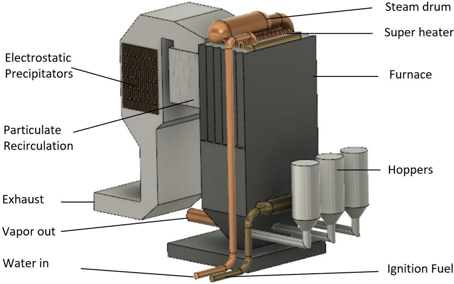
Figure 2. 3D CAD model of a boiler and its corresponding components.
2.1.1. Model scale
Once the CAD model of the power plant to be inspected is obtained, it is appropriately scaled down to fit the software working environment. We define the model scale
 $S_L$
as the ratio of length of the facility
$S_L$
as the ratio of length of the facility
 $L_p$
to the length of the CAD model
$L_p$
to the length of the CAD model
 $L_m$
.
$L_m$
.
 \begin{equation}S_L=\frac{L_p}{L_m} \end{equation}
2.2. System description
2.2.1. Camera field of view
For a chosen dimension d, and effective focal length f, the angular field of view
 $\alpha$
can becalculated as,
$\alpha$
can becalculated as,
 \begin{equation}\alpha =2\arctan\left(\frac{d}{2f}\right) \end{equation}
The camera field of view can be measured horizontally, vertically, and diagonally (Fig. 3). For an Intel Real®Sense R200 camera, the horizontal
 $\alpha_h$
vertical
$\alpha_h$
vertical
 $\alpha_v$
diagonal
$\alpha_v$
diagonal
 $\alpha_d$
angular field of view for the RGB camera, are 60°, 45° and 70°, respectively [Reference Keselman, Woodfill, Grunnet-Jepsen and Bhowmik24].
$\alpha_d$
angular field of view for the RGB camera, are 60°, 45° and 70°, respectively [Reference Keselman, Woodfill, Grunnet-Jepsen and Bhowmik24].

Figure 3. UAV inspection camera angular FOV (field of view).
2.2.2. The UAV system
The aerial platform used in this project consists of an off-the shelf quadrotor vehicle Intel® Aero Ready to Fly Drone (Fig. 4). However, this paper focuses on the offline trajectory generation and validation in a simulation environment to show the capabilities of the approach. All data and parameters are taken from the said UAV system for the corresponding calculations.

Figure 4. Drone platform and reference frames.
2.3. UAV modeling and control
2.3.1. UAV kinematics
To analyze the motion of the drone, an inertial frame {A} (or world frame) and a body coordinate frame {B} are included. {A} is selected at a convenient location that acts as the global reference for the plant to be inspected. In the other hand, {B} has its origin coincident with the center of gravity of the quadrotor, the z axis downward, and the x axis in the direction of the flight, following the aerospace convention (Fig. 4). Besides, as depicted in Fig. 5, the position of the drone in inertial frame {A} is given by the vector
 $\boldsymbol{r}\in\mathbb{R}^{3}$
.
$\boldsymbol{r}\in\mathbb{R}^{3}$
.

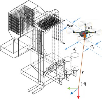
Figure 5. Kinematic Diagram: frames definition and inspection distances in a power plant boiler case study.
The inspection cameras on the UAV are installed in the chassis and are near the depth sensors; therefore, the camera location can be considered as the point of origin/zero point for the drone. Notably, the UAV propellers expand beyond this point by
 $a_d$
and from the extreme endpoint of the propeller to the closest point on the inspection surface can be designated as
$a_d$
and from the extreme endpoint of the propeller to the closest point on the inspection surface can be designated as
 $d_s$
. As such, the total inspection offset from camera at any time is
$d_s$
. As such, the total inspection offset from camera at any time is
 \begin{equation}\ d =d_{s}+a_{d} \end{equation}
For a safe flight path planning, a minimum drone offset distance
 $d_s$
is introduced. Also, due to the design of the drone, the rotor blades expand a certain distance from the camera that also needs to be considered along with the camera focal distance itself. Therefore, the offset distance should be
$d_s$
is introduced. Also, due to the design of the drone, the rotor blades expand a certain distance from the camera that also needs to be considered along with the camera focal distance itself. Therefore, the offset distance should be
 $d \geq d_s+a_d$
and
$d \geq d_s+a_d$
and
 $d>f$
at any time (Fig. 5). As such, the position vector for the UAV camera is
$d>f$
at any time (Fig. 5). As such, the position vector for the UAV camera is
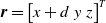 \begin{equation} {{\boldsymbol{r}} } = \begin{bmatrix} x+d & y & z \end{bmatrix}^{T}\end{equation}
For a quadrotor, the angular motion state about the three rotation axes is represented by six state variables: the angular velocity vector,
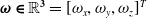 $\boldsymbol{\omega\in\mathbb{R}^{3}}=[\omega_x, \omega_y, \omega_z]^T$
about the three axes of the body frame and the Euler angles
$\boldsymbol{\omega\in\mathbb{R}^{3}}=[\omega_x, \omega_y, \omega_z]^T$
about the three axes of the body frame and the Euler angles
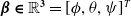 $\boldsymbol{\beta\in\mathbb{R}^{3}}=[\phi,\theta,\psi]^T$
, representing the roll, pitch and yaw angles, respectively. The 3-2-1 (Z-Y-X) Euler angles are used to model the rotation of the quadrotor in the global frame. The rotation matrix for transforming the coordinates from {A} to {B} is given by the rotation matrices about each axis (
R
′
$\boldsymbol{\beta\in\mathbb{R}^{3}}=[\phi,\theta,\psi]^T$
, representing the roll, pitch and yaw angles, respectively. The 3-2-1 (Z-Y-X) Euler angles are used to model the rotation of the quadrotor in the global frame. The rotation matrix for transforming the coordinates from {A} to {B} is given by the rotation matrices about each axis (
R
′
 $(\phi)$
,
R
′
$(\phi)$
,
R
′
 $(\theta)$
, and
R
′
$(\theta)$
, and
R
′
 $(\psi)$
). Therefore, the rotation matrix
$(\psi)$
). Therefore, the rotation matrix
 $\boldsymbol{R}\in\mathbb{R}^{3 \times 3}$
that expresses the orientation of the coordinate frame {B} with respect to global reference frame {A} is obtained.
$\boldsymbol{R}\in\mathbb{R}^{3 \times 3}$
that expresses the orientation of the coordinate frame {B} with respect to global reference frame {A} is obtained.
 \begin{equation} \boldsymbol{R} = \boldsymbol{R}'{\rm (\phi)} \boldsymbol{R}'(\theta) \boldsymbol{R}'(\psi) = \begin{bmatrix} C_\theta C_\psi & C_\theta C_\psi & -S_\theta \\[4pt] S_\phi S_\theta C_\psi & C_\phi C_\psi + S_\phi S_\theta S_\psi & S_\phi C_\theta \\[4pt] C_\phi S_\theta C_\psi + S_\phi C_\psi & C_\phi S_\theta C_\psi - S_\phi C_\psi & C_\psi C_\theta \end{bmatrix}\end{equation}
where
 $ C_\phi $
and
$ C_\phi $
and
 $ S_\phi $
are abbreviations of cos(
$ S_\phi $
are abbreviations of cos(
 $\phi$
) and sin(
$\phi$
) and sin(
 $\phi$
), respectively, similarly for
$\phi$
), respectively, similarly for
 $\theta$
and
$\theta$
and
 $\psi$
. The components of angular velocity of the quadrotor,
$\psi$
. The components of angular velocity of the quadrotor,
 $\omega_x$
,
$\omega_x$
,
 $\omega_y$
and
$\omega_y$
and
 $\omega_z$
are related to the derivatives of the roll, pitch and yaw angles as,
$\omega_z$
are related to the derivatives of the roll, pitch and yaw angles as,
 \begin{equation} \begin{bmatrix} \omega_x \\[4pt] \omega_y \\[4pt] \omega_z \end{bmatrix} = \begin{bmatrix} 1 & 0 & -S_\theta \\[4pt] 0 & C_{\phi} & S_{\phi} C_\theta \\[4pt] 0 & - S_{\phi} & S_{\phi} \end{bmatrix} \begin{bmatrix} \dot{\phi} \\[4pt] \dot{\theta} \\[4pt] \dot{\psi} \end{bmatrix}\end{equation}
2.3.2. UAV dynamics
The four rotors on the quadrotor are driven by electric motors powered by electric speed controllers. The rotor speed is
 $\overline{\omega_{i,}}$
and the thrust is an upward vector,
$\overline{\omega_{i,}}$
and the thrust is an upward vector,
 \begin{equation}T_i = b \overline{\omega_i}, \quad i = 1,2,3,4 \end{equation}
In the quadrotor’s negative z-direction, where b
 $>$
0 is the lift constant, dependant on number of blades, air density, the cube of the rotor blade radius and the chord length of the blade. Assuming the quadrotor is a symmetric rigid body, its equations of motion can be written as [Reference Corke25],
$>$
0 is the lift constant, dependant on number of blades, air density, the cube of the rotor blade radius and the chord length of the blade. Assuming the quadrotor is a symmetric rigid body, its equations of motion can be written as [Reference Corke25],
 \begin{equation}\boldsymbol{f}= \boldsymbol{f}_g + T \end{equation}
 \begin{equation} \boldsymbol{\tau} = \boldsymbol{J}{\boldsymbol{\dot\omega}} + \boldsymbol{\omega} \times \boldsymbol{J}\boldsymbol{\omega}\end{equation}
where
 $\boldsymbol{f}\in\mathbb{R}^3$
and
$\boldsymbol{f}\in\mathbb{R}^3$
and
 $\boldsymbol{\tau}\in\mathbb{R}^{3}$
are the force and torque applied to the vehicle, respectively;
$\boldsymbol{\tau}\in\mathbb{R}^{3}$
are the force and torque applied to the vehicle, respectively;
 $\boldsymbol{J}\in\mathbb{R}^{3\times 3}$
is the inertia matrix of the quadrotor, and
$\boldsymbol{J}\in\mathbb{R}^{3\times 3}$
is the inertia matrix of the quadrotor, and
 $\boldsymbol{\omega}\in\mathbb{R}^3$
is the angular velocity vector of the UAV,
$\boldsymbol{\omega}\in\mathbb{R}^3$
is the angular velocity vector of the UAV,
 $f_g$
is the force due to the gravity, and T is the total thrust generated by the propellers. The resultant force can be then expressed as
$f_g$
is the force due to the gravity, and T is the total thrust generated by the propellers. The resultant force can be then expressed as
 \begin{align} \boldsymbol{f} &= \begin{bmatrix} 0 \\[4pt] 0 \\[4pt] mg \end{bmatrix} + \boldsymbol{R} \times \begin{bmatrix} 0 \\[4pt] 0 \\[4pt] T_1 + T_2 + T_3 + T_4 \end{bmatrix}\end{align}
Pairwise differences in rotor thrusts cause the vehicle to rotate. The rolling torque about the vehicle’s x axis is generated by the moments
 \begin{equation} \tau_x = a_{CM} T_4 - a_{CM} T_2 \end{equation}
 $a_{CM}$
is the distance from the quadrotor center of mass to the rotor axis (Fig. 5). Converting the equation in terms of rotor speeds using (7)
$a_{CM}$
is the distance from the quadrotor center of mass to the rotor axis (Fig. 5). Converting the equation in terms of rotor speeds using (7)
 \begin{equation}\tau_x = a_{CM} b (\overline{\omega_4}^2 - \overline{\omega_2}^2) \end{equation}
Similarly, for the torque about its y axis,
 \begin{equation}\tau_y = a_{CM} b (\overline{\omega_1}^2 - \overline{\omega_3}^2) \end{equation}
The torque applied to each propeller by the motor needs to overcome the aerodynamic drag,
 \begin{equation}{Q}_{i} = k \overline{\omega_i}^2 \end{equation}
where k depends on the same factors as b. From the torque, a reaction torque on the airframe is transmitted that is responsible for the “yaw” torque about the propeller shaft in the opposite direction to its rotation. The total torque about z axis is
 \begin{align} \begin{aligned}\tau_z &= Q_1 - Q_2 + Q_3 -Q_4 \\[4pt] &= k(\overline{\omega_1}^2 - \overline{\omega_2}^2 +\overline{\omega_3}^2 -\overline{\omega_4}^2)\end{aligned} \end{align}
where the signs are different due to the rotation directions (counter clockwise taken as positive for rotor 1 and 3) of the rotors. Therefore, yaw rotation is achieved by carefully controlling all of the 4 rotor speeds. The applied torque
 $\boldsymbol{\tau}$
is calculated from (12), (13), (15) and (7) obtaining
$\boldsymbol{\tau}$
is calculated from (12), (13), (15) and (7) obtaining
 \begin{align} \boldsymbol{\tau} &= \begin{bmatrix} \tau_x \\[4pt] \tau_y \\[4pt] \tau_z \end{bmatrix}=\begin{bmatrix} a_{CM}b(\overline{\omega_4}^2 - \overline{\omega_2}^2) \\[4pt] a_{CM}b(\overline{\omega_1}^2 - \overline{\omega_3}^2) \\[4pt] k(\overline{\omega_1}^2 - \overline{\omega_2}^2 +\overline{\omega_3}^2 -\overline{\omega_4}^2) \end{bmatrix} = \boldsymbol{J}{\boldsymbol{\dot \omega}} + \boldsymbol{\omega}\times \boldsymbol{J} \boldsymbol{\omega} \end{align}
By combining Eqs. (7) and (10), the following expression is obtained
 \begin{align} \begin{bmatrix} T \\[4pt] \boldsymbol{\tau} \end{bmatrix} &= \begin{bmatrix} -b & -b & -b & -b \\[4pt] 0 & -a_{CM}b & 0 & a_{CM}b\\[4pt] a_{CM}b & 0 & -a_{CM}b & 0\\[4pt] k & -k & k & -k \end{bmatrix} \begin{bmatrix} \overline{\omega_1}^2 \\[4pt] \overline{\omega_2}^2 \\[4pt] \overline{\omega_3}^2 \\[4pt] \overline{\omega_4}^2 \end{bmatrix} = \boldsymbol{A} \begin{bmatrix} \overline{\omega_1}^2 \\[4pt] \overline{\omega_2}^2 \\[4pt] \overline{\omega_3}^2 \\[4pt] \overline{\omega_4}^2 \end{bmatrix}\end{align}
The moments and the forces of the quadrotor are function of the rotor speeds. The matrix A is constant, and the equation can be rewritten using matrix inversion for obtaining the rotor speeds given the torques and forces [Reference Corke25],
 \begin{align} \begin{bmatrix} \overline{\omega_1}^2 \\[4pt] \overline{\omega_2}^2 \\[4pt] \overline{\omega_3}^2 \\[4pt] \overline{\omega_4}^2 \end{bmatrix} = \boldsymbol{A}^{-1} \begin{bmatrix} T \\[4pt] \tau_{x} \\[4pt] \tau_{y} \\[4pt] \tau_{z} \end{bmatrix}\end{align}
2.3.3. UAV control system
As depicted in Fig. 6, the UAV position and attitude are controlled by a series of controllers built-in in the system. A position controller receives the desired coordinates to track in the position vector set-point
 $\boldsymbol{r}_{sp}\in\mathbb{R}^{3}$
that is compared with the actual estimated drone position
$\boldsymbol{r}_{sp}\in\mathbb{R}^{3}$
that is compared with the actual estimated drone position
 $\boldsymbol{\hat{r}}\in\mathbb{R}^{3}$
to obtain the position error
$\boldsymbol{\hat{r}}\in\mathbb{R}^{3}$
to obtain the position error
 $\boldsymbol{\tilde{r}}\in\mathbb{R}^{3}$
to compensate for. The desired coordinates are the final coordinates obtained from the “Post-processing/toolpath extraction phase.” The UAV’s X, Y and Z axis are set via the flight controller, inline with the AM/CAM software, and the origin of the inertial frame, {A}, (Fig. 5) is where the UAV is placed to start the aerial inspection flight. A proportional controller calculates then the desired velocity
$\boldsymbol{\tilde{r}}\in\mathbb{R}^{3}$
to compensate for. The desired coordinates are the final coordinates obtained from the “Post-processing/toolpath extraction phase.” The UAV’s X, Y and Z axis are set via the flight controller, inline with the AM/CAM software, and the origin of the inertial frame, {A}, (Fig. 5) is where the UAV is placed to start the aerial inspection flight. A proportional controller calculates then the desired velocity
 $\boldsymbol{v}_{sp}\in\mathbb{R}^{3}$
that is limited according to the hardware capabilities. Then, a PID controller in cascade will determine the required thrust T to achieve the desired altitude. While, through a conversion stage, the thrust and the desired yaw angle
$\boldsymbol{v}_{sp}\in\mathbb{R}^{3}$
that is limited according to the hardware capabilities. Then, a PID controller in cascade will determine the required thrust T to achieve the desired altitude. While, through a conversion stage, the thrust and the desired yaw angle
 $\psi_{sp}$
determine the desired attitude
$\psi_{sp}$
determine the desired attitude
 $\boldsymbol{\beta}_{sp}\in\mathbb{R}^{3}$
that is compared with the estimated attitude
$\boldsymbol{\beta}_{sp}\in\mathbb{R}^{3}$
that is compared with the estimated attitude
 $\boldsymbol{\hat{\beta}}\in\mathbb{R}^{3}$
to obtain the orientation error
$\boldsymbol{\hat{\beta}}\in\mathbb{R}^{3}$
to obtain the orientation error
 $\boldsymbol{\tilde{\beta}}\in\mathbb{R}^{3}$
that will be compensated by a proportional controller, leading to the attitude rate set point
$\boldsymbol{\tilde{\beta}}\in\mathbb{R}^{3}$
that will be compensated by a proportional controller, leading to the attitude rate set point
 $\boldsymbol{\dot{\beta}}_{sp}\in\mathbb{R}^{3}$
that at the same time is related to the estimated attitude rate
$\boldsymbol{\dot{\beta}}_{sp}\in\mathbb{R}^{3}$
that at the same time is related to the estimated attitude rate
 $\boldsymbol{\dot{\hat{\beta}}}\in\mathbb{R}^{3}$
to determine the attitude rate error
$\boldsymbol{\dot{\hat{\beta}}}\in\mathbb{R}^{3}$
to determine the attitude rate error
 $\boldsymbol{\dot{\tilde{\beta}}}\in\mathbb{R}^{3}$
that will be regulated by a PID controller that generates the control torques, that together with the thrust command the drone to the desired position and orientation. Finally, the required motor’s angular speed can be calculated by (18). References [finite] and [global] The estimated attitude and attitude rates are directly inferred from the IMU data, while the position estimation is more complex and cannot rely on a GPS signal. For solving this issue, we propose implementing a well-tested visual inertial odometry (VIO)-based sub-system [Reference Nikolic, Burri, Rehder, Leutenegger, Huerzeler and Siegwart7] using a stereo camera integrated in the payload. As for the simulation, the actual UAV’s position is corrupted by noise, which simulates the VIO system’s output working in a feature richenvironment.
$\boldsymbol{\dot{\tilde{\beta}}}\in\mathbb{R}^{3}$
that will be regulated by a PID controller that generates the control torques, that together with the thrust command the drone to the desired position and orientation. Finally, the required motor’s angular speed can be calculated by (18). References [finite] and [global] The estimated attitude and attitude rates are directly inferred from the IMU data, while the position estimation is more complex and cannot rely on a GPS signal. For solving this issue, we propose implementing a well-tested visual inertial odometry (VIO)-based sub-system [Reference Nikolic, Burri, Rehder, Leutenegger, Huerzeler and Siegwart7] using a stereo camera integrated in the payload. As for the simulation, the actual UAV’s position is corrupted by noise, which simulates the VIO system’s output working in a feature richenvironment.

Figure 6. UAV controllers for position and attitude control.
2.4. Toolpath generation methods
The introduced method proposes to obtain the flight path of the drone from the path that a CNC Machine tool or Nozzle’s 3D printer would follow. Therefore, two approaches are used, that is, CAM and AM method. For both methods, the toolpath is set with a predetermined offset for the drone to avoid collision and safe inspection flight, which was carefully calculated in the previous step. Using a CAD/CAM software package, the toolpath data for the machining operation are created, by obtaining the nodal coordinates which are on the path of the cutter as well as the tool feed rate, type of motion and type of the operation such as milling. Essentially, a path that is followed in a CAM milling operation and a 3D printer (in AM) are very similar, one being subtractive as the tool travels in −Z axis (top to bottom) and the other being additive, that is, the tool travels in +Z axis (bottom to top). During the operation of both manufacturing methods, the tool moves layer by layer. These paths are similar to the flighting path followed by an UAV, encompassing a structure to be inspected, with an appropriate offset. Either of the manufacturing methods, CAM or AM, can be used to generate the UAVtrajectory.
In CAM milling operations, the cutter follows a path, for example, a zigzag path or a peripheral path depending on the pre-set global parameters such as tool cutting radius, depth of cut, and stepover cut, which correspond to flight path layer to layer distance, the flight path overlaps needed for generating a good quality inspection photography, etc. In 3D AM operation, the deposition head or extruder moves along +Z direction, that is, it moves from bottom to top, layer by layer. Therefore, if the signs of the Z-coordinates in the G-code file for AM are reversed, it will yield a CAM operation path file. Although the sign conversion would need targeted programming, both methods have a similar basic idea. In the case of UAV trajectory, either of the approaches can be used.
2.5. Post-processing (Toolpath extraction)
In the “Post-Process” option, the XYZ coordinates are exported from G-code, which are files with detailed machine instruction that not only contain the required tool end point or nodal coordinates, types of the motions, and necessary instructions but also contain information such as different cutting modes, type of tool, tool change, tool speed, cutting direction, tool orientation, operation and other important information specific to the type of manufacturing machines. However, all information is not needed in this project for generating a UAV trajectory. Therefore, for using this file format, unnecessary data must be cleared from the file. Post-process is done in two ways. First, a software add-on is used for 3 axis milling operation in the CAM-based method to directly extract the coordinates. Second, G-code-specific programming is done for both CAM and AM methods to extract the same.
2.6. Trajectory generation and UAV inspection simulation
Both coordinate extraction methods output a set of coordinates that represent the tool end points in 3D space. These coordinates are given timesteps and processed to generate a trajectory or a flight path of the UAV for powerplant inspection. These flightpaths are tested by two simulation software: MATLAB SIMULINK and using the PX4 Autopilot with Gazebo virtual simulator.
3. Simulation Study
3.1. CAD model
3.1.1. Model scaling
Boiler height commonly ranges between 12–30 m. For this study, a 17 m high boiler is designed. Due to the tool size limitation, overall power plant height is scaled down to 170 mm. Therefore, model scale
 $(S_L)$
is 100:1. The
$(S_L)$
is 100:1. The
 $S_L$
is good for all use cases, including actual case scenario of a real-life boiler height range (typically 12-30m). The AM tool ’‘Slicer’’ is also good for scaling and trajectory planning of Z axis from 120-300 mm range. Once trajectory planning is done in model phase, the coordinates or the UAV waypoints is converted to the real-life scaling using the scale of 100:1, such that a 100 mm model distance between coordinates converts to 10 m in actual use.
$S_L$
is good for all use cases, including actual case scenario of a real-life boiler height range (typically 12-30m). The AM tool ’‘Slicer’’ is also good for scaling and trajectory planning of Z axis from 120-300 mm range. Once trajectory planning is done in model phase, the coordinates or the UAV waypoints is converted to the real-life scaling using the scale of 100:1, such that a 100 mm model distance between coordinates converts to 10 m in actual use.
3.1.2. Camera field of view
For calculation, the stereo camera angle of view is taken. Average camera focal length is 30 mm. Here, a 500 mm inspection offset distance for UAV camera is chosen. From (2), with
 $\alpha_{h} = 60^{\circ}$
,
$\alpha_{h} = 60^{\circ}$
,
 $\alpha_{v} = 45^{\circ}$
, and
$\alpha_{v} = 45^{\circ}$
, and
 $f = 5$
mm, the inspection grid horizontal length, h, and vertical length, v, are calculated:
$f = 5$
mm, the inspection grid horizontal length, h, and vertical length, v, are calculated:
 \begin{equation}h = 2f\tan\frac{\alpha_h}{2}\! \Rightarrow h = 5.8\end{equation}
 \begin{equation}v = 2f\tan\frac{\alpha_v}{2}\! \Rightarrow v = 4.1\end{equation}
Considering a 30% overlap of adjacent pictures for a sharp and high image quality inspection profile, the camera inspection field of view is taken as,
 \begin{equation}h_1 = 70\% of h = 4.06 \approx 4 \end{equation}
 \begin{equation}v_1 = 70\% of v = 2.87 \approx 2.5 \end{equation}
Therefore, the model scale yields to vertical length field of view (
 $v_1$
) of 2.5 mm; hence, this is the maximum step down/feed for CAM and layer to layer height in AM. From the scale ratio, the application field of view is calculated to be 400 mm
$v_1$
) of 2.5 mm; hence, this is the maximum step down/feed for CAM and layer to layer height in AM. From the scale ratio, the application field of view is calculated to be 400 mm
 $\times$
250 mm approximately (Fig. 7) and the number of parallel toolpath (slices) is 68.
$\times$
250 mm approximately (Fig. 7) and the number of parallel toolpath (slices) is 68.

Figure 7. UAV camera FOV (field of view) grid.
3.1.3. Drone velocity range
Velocity of drones range from 10 mph to as high as 70 mph. For this project, an average speed needs to be calculated. Average drones used for photography usually clock between 30–50 mph, for which the drone camera must have a suitable fps (frames per second) value. For the maximum speed,
 $v_{max} =$
50 mph
$v_{max} =$
50 mph
 $= 22.235 $
m/s, the frame per second (fps) for the drone camera is the ratio of total distance to the camera grid horizontal length
$= 22.235 $
m/s, the frame per second (fps) for the drone camera is the ratio of total distance to the camera grid horizontal length
 $(h_1)$
 \begin{align} \begin{aligned} {\rm fps} & = \frac{22,352}{400} \\ &= 55.88 \end{aligned} \end{align}
Taking an average speed of 20 mph or 8.9408 m/s, that is, the drone would need to travel 8940.8 mm in 1 sec. Therefore,
 \begin{align}\begin{aligned} {\rm fps} &= \frac{8940.8}{400} \\ &= 22.352 \end{aligned} \end{align}
The proposed camera has 60 fps for a depth resolution of
 $480\times360$
, which is well within our calculated range. Also, as mentioned previously, a 30% overlap has been accounted for a higher image quality. As such, both photography and video for inspection can be used well with the inspection payload for an average drone speed of 20 mph.
$480\times360$
, which is well within our calculated range. Also, as mentioned previously, a 30% overlap has been accounted for a higher image quality. As such, both photography and video for inspection can be used well with the inspection payload for an average drone speed of 20 mph.
3.2. Toolpath generation
3.2.1. Method 1: CAM toolpath generation
A. Toolpath Generation with 2D Contour Operation: In the “Manufacture” workspace of Fusion 360, the machining properties are setup, that is, setting up the appropriate operation type, defining work coordinate system, choosing apt stock offset, post-processing setup, etc.
At first, a relevant sized stock block is chosen. The stock offset is equal to the inspection offset, “d” (Eq. (3)). In order to optimize the toolpath and thereby obtaining a proper UAV flight trajectory, the toolpath needs to be uniformly distributed and well wrapped around the model (Fig. 8). As such, a 2D contour milling operation in the CAM environment of the Fusion 360 software is selected. All machining parameters are aptly chosen which gives a uniform toolpath around the powerplant (Table I). The endpoint of a 2.5 mm diameter ball end point cutting tool chosen for this operation, machines out the part from the stock and a “toolpath’’ is obtained.

Figure 8. Toolpath generated around the powerplant CAD model for 2D contour operation.
Table I. CAM Contour (2D) machining parameters.

Two very important parameters are maximum step down and stock offset. “Maximum step down” parameter represents the length that is traveled when the cutting tool goes to next layer, and this corresponds to the hatch distance value in AM (slice). “Stock offset” parameter corresponds to the vertical distance from the inspection surface which is correlated to the distance of the camera to capture inspection profile photos and videos. These parameters are recommended considering the minimum and smallest distance value that can result in dense inspection profile; however, different values can be set for these parameters as operation requires. For example, here a minimum safe distance is taken as500 mm, but it can be increased depending on the type of UAV and the capability of its camera for producing desired outcome.
Mentionable is that the ‘‘blue’’ path lines describe cutting the stock or machining while the ‘‘yellow’’ and ‘‘red’’ path lines describe tool retraction and ramping, respectively. Notably, due to the tool orientation, the overhang, gaps and inward slopes are avoided, as expected from a CAM operation. Although the parallel toolpath around the inward slope of the exhaust is acceptable due to the camera’s superior zoom capabilities, however, to get the best possible wrapped toolpath of the section, tool orientation is changed.
B. Toolpath Generation with Modified Tool Orientation: For the inner gap of the powerplant model, again 2D contour milling operation is chosen, other parameters are the same (Table II). The Z axis of the tool orientation along with Y axis are flipped 180° (Fig. 9(a)). Z axis directs the tool entry to the workpiece. For this case, it is the same as assuming that the workpiece has been flipped for operating from the bottom surface of the setup, whereas the X axis is setup according to the manufacture operation coordinate principle. The inner gap between the boiler and exhaust can also be addressed with “Slot” milling operation (Fig. 9(b)). This is a step toolpath that requires a different set of parameters (Table II).
Table II. CAM Slot machining parameters.


Figure 9. Toolpaths generated with modified tool orientation and operation for the component gap and inward slope of the powerplant CAD model.
Like the earlier operation, Z axis is pointing downwards (flipped). Although the toolpath is able the reach the shallow gap on the upper chamber of the exhaust, due to the aerodynamic restriction of a UAV, it is not considered and the operation ceases near the shallow zone of the “particulate recirculation” component of the power plant.
Overall for all operations, ‘‘smooth transition’’ and ‘‘plunge in’’ features were chosen to avoid sharp change in UAV flight heading. From the generated toolpath, additional noise is observed for the CNC tool safe retrievals/lead-ins/lead-outs. Mentionable is that the tool time information, for example, feed rate, revolution, surface speed, is not used in the final flightpath generation. Only the tool end point coordinates are extracted as point cloud; therefore, these are not essential to this project. Later, an UAV appropriate timestep is set up.
3.2.2. Method 2: AM extruder path
In order to obtainthe external coordinates with a pre-set offset, a CAM-based approach was used previously. The CAM base method has some challenges that are inherent to the CAM characteristics, for example:
-
1. Machining of certain features is difficult, for example, inward slopes larger than 45, convex surfaces, etc.
-
2. Difficult to reach shallow gaps between design parts due to tool size limitation. The tool tilt angle is also limited due to physical constraint and workpiece orientation etc.
To overcome these challenges, an “Additive Manufacture (AM)”-based method is introduced with significant advantages. Essentially, a path that is followed in a CAM milling operation and a 3D printer (in AM) is very similar, one being subtractive, tool traveling in -Z axis (top to bottom) and the other being additive, that is, tool travels in +Z axis (bottom to top) (Fig. 10). During the operation of both manufacturing methods, the tool moves one layer at a time.

Figure 10. 3D printing layers preview of the model in Cura 3.6.0.
A commercially available 3D printer software (slicer) “Ultimaker Cura 3.6.0” is used to generate a 3D shell of the power plant with a pre-set offset equal to 5 mm, similar to CAM method (Table III). The layer height corresponds to the vertical travel of the UAV during inspection. No structure support is chosen, and mostly default parameters have been opted for getting a general shape of the powerplant. This operation gives extruder/toolpath coordinates at the selected offset or the shell itself. This covers all surface areas, including the shallow gaps and slopes. The G-code generated a bottom to upward Z axis values, along with XY coordinates, layer by layer (Fig. 10). Considering all the advantages in the final trajectory generation, the AM method is finalized for use.
Table III. AM parameters.

3.3. Exporting toolpath coordinates
3.3.1. Direct data extraction
Using a post-process add-on, the Cartesian coordinates of the tool endpoints are exported (Fig. 11). This is the first step of path planning. There are 109,575 number of points in the ‘‘exhaust’’ component of the powerplant setup alone. The point cloud is very dense; hence, a snapshot of the coordinates is shown (Fig. 11). In this step, all the points are taken and organized under one global coordinate. In the second and third operations, tool axis, that is, Z axis and Y axis, was flipped. In this step, the negative Z and Y coordinate point values are overturned, and the data are reset and arranged with Z values going low to high in a CSV file. Mentionable, this method can only be used for 3 axis milling operations.

Figure 11. A sample of the initial Cartesian coordinates (xyz) exported in excel sheet as. csv file.
3.3.2. Targeted G-code decoding with MATLAB
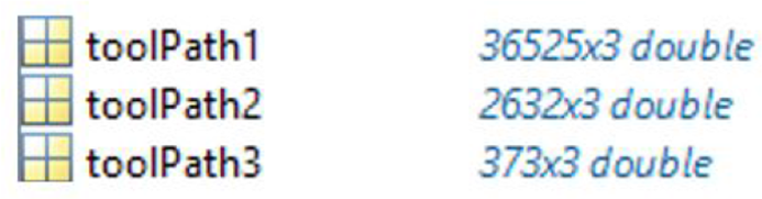
Both CAM and AM methods essentially send instructions in a coded format to the machine (CAM/CNC/3D printers) it needs to run, called the G-code files. As mentioned earlier, G-code files with detailed machine instruction not only contain the required nodal coordinates but also other necessary instructions specific to a CNC or a 3D printer to operate it safely. As such, G-codes vary depending on the machine it is programming to run, that is, machine-specific. Using MATLAB coding, specifically targeted to the G-Code type (CAM/AM), the tool end point coordinates are extracted discarding all other information. At first, only the ‘‘exhaust’’ component is studied, and then, the full powerplant model is used which gives a dense plot of
 $36525\times3$
double points, that includes all the tool end point coordinates (Fig. 12(a)).
$36525\times3$
double points, that includes all the tool end point coordinates (Fig. 12(a)).
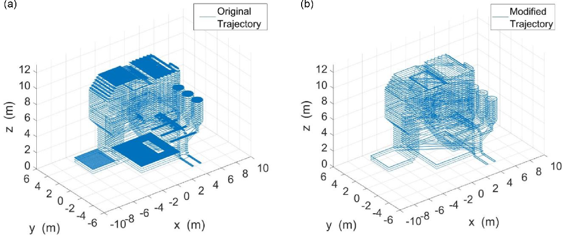
Figure 12. Coordinates obtained from a G-Code (AM method) of the power plant using MATLAB.
3.3.3. Toolpath/Trajectory modification
Although the targeted programming successfully extracts the coordinates, the number points is very dense as is expected from a 3D printer slicer generated G-Code (Fig. 12(a)). There is also variation of point cloud density, for example, the flat horizontal surfaces have denser point clouds than the other parts. To reduce the number of points, to get rid of noise and also to get a uniform external trajectory pattern without any conflict with the plant surface mesh, MATLAB code is modified that gives an updated trajectory (Fig. 12(b)). However, the arbitrary jump from one layer to another give trajectory lines through the surface mesh itself. Also, the support generation at the bottom of the structure remains which is unnecessary.
Trajectory is further modified, and an improved trajectory is achieved that has significantly smaller number of points (373x3 double) as well as a conflict-free trajectory (Fig. 13). Also, the significant reduction of point cloud (almost 1/100th) will result in better trajectory and computationally less expensive when fed to the inspection UAV (Fig. 14).

Figure 13. Final modified trajectory the power plant obtained using MATLAB programming.

4. Trajectory Generation for UAV Inspection
The AM method of coordinate extraction is used to plot the UAV trajectory of the power plant with MATLAB (Fig. 15). Here the black lines correspond to the surface STL mesh and the blue lines depict the trajectory. In comparison, the trajectory generated with the AM method is much smoother, uniform and covers all surfaces no matter the geometry. As such, AM method is preferred over the first method using CAM.

Figure 15. Flight path generated in MATLAB for AM method.
Mentionable is that, after a period of operation of the power plant, there may be some discrepancies between the original CAD model and the real setup, for example, loose pipes and hanging wires. To avoid such deviation and avoid collision, the UAV will use an anti-collision mechanism taking advantage of the onboard sensors. The projected trajectory is virtually validated by simulation.
5. Simulation
PX4 is a professional autopilot, that is, the flight stack software for controlling UAVs that implements different flight modes and safety features, and it is widely used on several drone platforms today. This software runs either on a flight controller, which is a computer on board of the drone or on a personal computer in the case of a simulation. PX4 offers different interfaces for interacting with the user: QGroundControl, a graphical interface to setup the drone, change parameters, create and execute flying missions, and visualize telemetry data in real time, and DronecodeSDK, a programming-defined API that provides the functions for interacting with the UAV. Moreover, Gazebo is a powerful robotics simulator that offers a 3D environment with a robust physics engine.
The chosen experimental setup consists on a general quadcopter model generated in the Gazebo simulator and running the PX4 flight stack, which shows us how a real drone would behave given the AM-generated coordinates. This validates our AM-based method for generating trajectories, as we prove that these paths can indeed be used to generate a real UAV flight mission. The proposed experimental methodology consists of the following:
-
1. Use a C++ program for reading the previously generated CSV file with the point coordinates that compose the trajectory.
-
2. Re-format as necessary and create mission items based on these points, using the DronecodeSDK libraries.
-
3. Upload and execute the mission on the simulated UAV.
-
4. Visualize the mission in real time using QGroundControl, while getting flight logs for an offline analysis of the UAV’s trajectory.
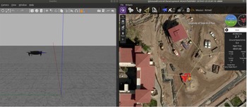
Thefirst experiment consists in executing a simple test trajectory for validating our setup, a test that simulates the hypothetical inspection of a cubic structure. The flight mission can be visualized in real time (Fig. 16), where we can see the actual drone’s flight in Gazebo, and the telemetry information using QGroundControl. At the same time, the logs are obtained using ROS, a framework for robotic applications, from where the estimated UAV position is later used for the offline analysis.

Figure 16. Gazebo simulation at runtime and QGroundControl plotting the UAV trajectory of the test mission in real time.
Moreover, Fig. 17 shows the estimated actual roll, pitch and yaw angles along with the set-point needed to achieve the desired trajectory, computed by the flight controller. These plots are obtained through the flight review logs in QGroundControl, and we can observe how the controller keeps good track of the set-point during the simulation. The same type of logs is going to be used when testing the real platform for visualizing the performance of the controllers and adjust them if needed.

Figure 17. Attitude tracking during the flight maneuver.
The actual AM-generated trajectory based on the power plant 3D model was used for creating the UAV’s flight mission. The same approach was followed, which allowed us to compare both trajectories (Figs. 18 and 19). The results show an adequate flight altitude during the test, with some variation but still a monotonically increasing trend. The top view of the flight path shows the general shape of the power plant, even if it is too smooth at some points due to the UAV cutting corners. The front and right views of the flight path are even closer to the AM-generated trajectory, showing some noise due to the flight controller corrections.

Figure 18. Comparison of: (a) the Z position of the tool based on (i) the AM, and (ii) the altitude of the UAV during flight, (b) the top view of both (i) the AM-generated trajectory, and (ii) the UAV inspection path.

Figure 19. Comparison of: (a) The front view of the (i) AM-generated trajectory, and (ii) the UAV flight path, (b) The right view of the (i) AM-generated trajectory, and (ii) the UAV flight trajectory.
Some shapes are lost, indicating that the post-processing of the coordinates is important to keep the relevant points for the flight mission. The 3D view of the trajectories in Fig. 20(a) and (b) shows side by side comparison of optimized trajectory obtained from AM method and the 3D view of the drone trajectory. The flight path follows the general shape of the power plant, even if it is too wavy and smooth at some points.
Furthermore, Fig. 20(c) shows the inspection flight path point cloud the drone follows using RVIZ visualization environment for ROS. For better realization, the point cloud is presented with and without the surface mesh of the boiler. Mentionable is, for better visualization, the number of points and layers have been reduced and optimized from the original AM tool generated point cloud, and as proof of concept of the adaptability and validity of this method.

Figure 20. Comparison of the (a) ideal inspection trajectory generated by AM and (b) the actual flight inspection path followed by the UAV and (c) inspection flight path point cloud visualized with the RVIZ environment with (left) and without (right) inspection surface (boiler).
Thenon-linearity/waviness and the offshoot from the ideal flight path are the result of the drone control parameters such as attitude control, gain, recovery and can be adjusted with drone engine in the simulation software. It is important to note that the PX4 mission parameters and the drone navigation can still be optimized for our application, and it does not negate the validity of this proposed method. The implementation of object detection and collision avoidance algorithms should allow the inspection paths to be closer to the real AM-generated trajectory, which will be explored in future work. Even in this case, the simulation results prove that the proposed approach for generating inspection paths based on the power plant 3D model can be indeed implemented using a real UAV controlled by a widely used professional flight stack.
6. Conclusion
This study introduced a novel method to inspect structural components of power plants using aerial robotics technology by generating flight paths similar to modern manufacturing techniques. Two approaches were considered, one based on the toolpath of a printer nozzle in AM and another is CAM. It is observed that the AM method offers better flight path generation characteristics because it is able to include small and difficult to access location. The proposed flight path generator seeks to enable very close inspection to capture more details in structurally complex environments with reduced flying areas, even in the absence of a GPS signal. Indeed, this approach would not be suitable for GPS-based navigation due to the precision required to localize the vehicle and because when inspecting the interior of a component GPS signal will not be available in most cases. The proposed method would need more than one flight to cover large areas due to the UAV flight time limitation. Simulations performed in the open-source 3D robotics simulator Gazebo demonstrated the feasibility of the method to construct drone offline trajectories. Due to the offline definition, this method would require a current CAD model of the system and the addition of obstacle detection and avoidance system to account for un-modeled objects or updates in the facility to inspect.
Acknowledgements
The authors would like to knowledge the financial support of the US Department of Energy (DOE) award No. DE-FE0031655.


 Open access