


Introduction
Dynamic models for calculating snow-avalanche motion have gained growing importance for avalanche hazard assessment in the last few years. Conversely the degree of precision required in hazard-mapping applications is far beyond that presently achievable by dynamic models. Substantial uncertainties characterize the definition of the avalanche starting conditions (release area and depth) and of the model parameters (friction coefficients). It is also the case that all dynamic models in common use are remarkably sensitive to both these types of input data. A detailed analysis on a group of dynamic models of hydraulic type, performed within the European Union Fourth Framework project SAME (Snow Avalanche Mapping and Warning Systems in Europe) (Reference Barbolini, Gruber, Keylock, Naaim and SaviBarbolini and others, 1998, Reference Barbolini, Gruber, Keylock, Naaim and Savi2000) has clearly shown that even relatively small variations of the friction coefficients (within 15%) can produce remarkable variations of the model output, in terms of either runout distance (up to the order of 102 m) or impact pressure (up to the order of 101 kPa at a fixed location). The sensitivity to release conditions was found to be lower, but sufficiently strong to obtain different mapping scenarios as a consequence of realistic variations of the release variables.
The uncertainties inherent in the model input-data specification, although well acknowledged, are usually not explicitly incorporated into the analysis and considered in the mapping results. These sources of error are normally addressed through conservative estimates of the parameters or, in some cases, by sensitivity analysis. However, each of these approaches has limitations for assessing the statistical implications of uncertainties. In the present paper some preliminary ideas are put forward for working in this direction in order to allow more appropriate risk assessment in avalanche-prone areas.
Method
A Monte Carlo approach to avalanche hazard mapping is proposed. The method combines statistically-based criteria for the evaluation of the input data of the dynamic models and deterministic avalanche modelling techniques. The uncertainties inherent in the use of dynamic models for mapping applications are explicitly accounted for by expressing the release variables and the friction coefficients in terms of “site-specific” probability distributions. These are then used to randomly generate samples of values for each model input, which are transformed into samples of mapping output by successive applications of the dynamic model. Thus, the mapping variables –– essentially runout distance and impact pressure –– are given in a form suitable for statistical analysis, and the effects of uncertainties can be formally considered in the hazard maps.
The specific methods introduced in order to estimate the site-specific frequency distributions for the release variables and for the friction coefficients are detailed in the rest of this paper. A brief presentation of the dynamic model used for avalanche calculations is given in the next section. In the concluding application, the hazard assessments are made according to the Swiss mapping criteria (Reference Salm, Burkard and GublerSalm and others, 1990).
Dynamic Model
The VARA avalanche computational models have been developed in the Hydraulic and Environmental Engineering Department of the University of Pavia since the early 1990s (Reference Natale, Nettuno, Savi and HamzaNatale and others, 1994; Reference NettunoNettuno, 1996; Reference Barbolini and HarbitzBarbolini, 1998). They use a hydraulic approach for the simulation of snow-avalanche flows; the equations are in fact similar to those originally derived and commonly applied for free-surface hydraulic flow simulations. Consequently, they are only applicable to dense snow avalanches.
According to Reference NettunoNettuno (1996), the unit-width one-dimensional equations for the conservation of mass and momentum of an avalanche flowing downslope can be written as follows:
where
![]() is the depth-averaged value for the downslope velocity component, h is the local flow depth, J is the dynamic friction coefficient, which incorporates the dissipation at the flow bed, and a is the local slope angle. Equations (1a) and (1b) are numerically integrated using an upwind second-order finite-volumes scheme (Reference NujicNujic, 1995).
is the depth-averaged value for the downslope velocity component, h is the local flow depth, J is the dynamic friction coefficient, which incorporates the dissipation at the flow bed, and a is the local slope angle. Equations (1a) and (1b) are numerically integrated using an upwind second-order finite-volumes scheme (Reference NujicNujic, 1995).
The form of the dynamic friction coefficient J is similar to the one first proposed by Reference VoellmyVoellmy (1955), with n2 equivalent to 1/ξ in the original Voellmy model:
μ is interpreted as a Coulomb friction at the flow bed, whereas the quadratic term may be interpreted with reference to the resistance developed in a granular material within the “inertial” flow regime (Reference BagnoldBagnold, 1954). However, in practical applications the friction coefficients μ and n are estimated by model calibration.
The unit-width version of the one-dimensional VARA model is appropriate for the description of flow on an open slope, which is the case for the avalanche path considered in this paper. As starting conditions this model requires a snow fracture height (HT in the following) and a longitudinal release length (Lr in the following).
Probability Distributions of Release Variables
Release depth
According to Reference Salm, Burkard and GublerSalm and others (1990), for given return period T and release-zone average altitude z the release depth HT(T, z) may be expressed as a function of the 3 day snow precipitation P72(T,z), the snowdrift overload PSD and the average slope of release zone 9 as follows:
where f(θ) is a slope factor, accounting for the reduction of released snow with increasing release-zone inclination. This paper explicitly considers the uncertainties in the determination of P72 (T, z) for an assigned return period and release-zone location by using suitable probability distributions. Equation (3) is then applied straightforwardly, with the values of f(θ) and PSD estimated according to the proposal of Reference Salm, Burkard and GublerSalm and others (1990).
The estimate of P72(T, z) is made on the basis of a regional analysis of the snowfall regime. The “index-value” technique is used for this purpose (Reference KiteKite, 1988). The data of different gauging stations from a given geographical area are made dimensionless (P*) by dividing by their average value. In this way, once the statistical homogeneity of the different stations has been checked by suitable tests (Reference KiteKite, 1988), all the recorded data can be put in a unique extended dimensionless sample. This data sample is then fitted to a generalized extreme-value (GEV) distribution (Reference Hosking, Wallis and WoodHosking and others, 1985; Reference Li-Hsiung and StedingerLi-Hsiung and Stedinger, 1992) so as to be able to estimate the values exceeded with various design probabilities, i.e. related to assigned return periods. By inversion of the GEV cumulative distribution function, the following expression for the quantile P7*2(T) can be derived (Reference Li-Hsiung and StedingerLi-Hsiung and Stedinger, 1992):
where a, b and k are scale, location and shape parameters of the distribution. Quantile estimators are random variables whose precision depends on the parent distribution, the parameter estimation method and the sample size. Following Reference Hosking, Wallis and WoodHosking and others (1985), the variance of the GEV/PWM (probability weighted moments) quantile estimator can be calculated from the following equation:
where N is the sample size and f(k, T) is an implicit algebraic function, whose values are tabulated in Reference Li-Hsiung and StedingerLi-Hsiung and Stedinger (1992).
Equation (4) is used to compute the mean value of the T-year event
![]() ; to define the confidence interval of this estimate, it is assumed that the estimation error is normally distributed, with standard deviation given by Equation (5).
; to define the confidence interval of this estimate, it is assumed that the estimation error is normally distributed, with standard deviation given by Equation (5).
The value of the 3 day precipitation at the location of interest (for selected T) is obtained by multiplying its dimensionless value P*(T) with the average 3 day precipitation at the altitude representative of the release zone
![]() This latter variable is estimated by linear regression of the average 3 day precipitation of different stations
This latter variable is estimated by linear regression of the average 3 day precipitation of different stations
![]() with their relative altitudes, which may be considered one of the most relevant parameters for explaining differences between snowfall records from separate gauges belonging to a given geographical area (Reference Salm, Burkard and GublerSalm and others, 1990). The regression error may be used as an appropriate error function. Thus, the values for
with their relative altitudes, which may be considered one of the most relevant parameters for explaining differences between snowfall records from separate gauges belonging to a given geographical area (Reference Salm, Burkard and GublerSalm and others, 1990). The regression error may be used as an appropriate error function. Thus, the values for
![]() are assumed to be normally distributed about the mean, with the standard deviation corresponding to the regression error.
are assumed to be normally distributed about the mean, with the standard deviation corresponding to the regression error.
Release length
The release length Lr is completely defined once the upper (Zu) and lower (Z{) release limits are located along the longitudinal path profile. Within the framework of the present paper, the uncertainties inherent in the definition of this release variable are explicitly taken into account by considering its lower limit Zx movable. This latter assumption does not appear to be too restrictive; in practical applications a high degree of uncertainty typically arises in the definition of the lower limit of release zones (the so-called “stauchwall”), whereas the identification of the upper limit is usually less problematic.
We propose to randomly locate Z, by means of a triangular probability distribution function (see Fig. 1), which represents one of the simplest ways to describe the variability of a quantity, accounting for a most probable value (
![]() in Fig. 1) and two limits (Zlmin and Z1Max in Fig. 1). The three parameters of the distribution (Zlmin, Zmax
and
in Fig. 1) and two limits (Zlmin and Z1Max in Fig. 1). The three parameters of the distribution (Zlmin, Zmax
and
![]() should be set on the basis of the specific topography of the considered release zone, as well as personal experience and/or knowledge of the site.
should be set on the basis of the specific topography of the considered release zone, as well as personal experience and/or knowledge of the site.

Fig. 1. Triangular probability distribution function for Z1.
Probability Distribution of Friction Coefficients
To date, the only reference table for friction coefficients that provides well-defined ranges in relation to the avalanche features (snow conditions, avalanche frequency) and path features (degree of channelling, vegetation) is that contained in the Swiss Guidelines (Reference Salm, Burkard and GublerSalm and others, 1990). However, as shown by Reference Barbolini, Gruber, Keylock, Naaim and SaviBarbolini and others (1998, Reference Barbolini, Gruber, Keylock, Naaim and Savi2000), these reference values, which result from the calibration of the Voellmy-Salm model, cannot be applied to other dynamic models, even if they use similar expressions for the flow resistance. Furthermore, these ranges have been demonstrated to be too wide to allow reasonable precision in the model results, given the sensitivity of the models (Reference Barbolini, Gruber, Keylock, Naaim and SaviBarbolini and others, 1998, Reference Barbolini, Gruber, Keylock, Naaim and Savi2000).
The alternative and usual procedure is to perform a direct “on-site” calibration of the model on the basis of suitably recorded historical events. Apart from the common lack of data on avalanche events appropriate for model calibration, it should also be noted that the release of a given snow volume can produce different runout distances depending on the released-snow characteristics and on the snow-cover properties along the track.
We suggest capturing such inherent variability, resulting from physical processes that are not explicitly modelled (e.g. erosion-deposition), by expressing the friction coefficients in terms of site-specific probability distributions that are also, in accordance with the Swiss Guidelines, assumed to be dependent on the avalanche frequency. Furthermore, to overcome the usual lack of site-specific avalanche data needed to infer these probability distributions, we propose to evaluate their parameters at a regional scale, i.e. by using friction coefficient values calibrated on different avalanche sites.
Model calibration
The model previously described has been calibrated against a group of adequate historical events (namely, with known release conditions and runout positions) related to avalanche sites belonging to separate regions within the Italian Alps, and representative of occurrences with different return periods. With regard to this latter aspect, the avalanche events are tentatively assigned to two general frequency classes: (a) relatively frequent events; (b) extremely rare events. A synthesis of model calibration is given in Table 1; more details can be found in Reference BarboliniBarbolini (1999).
Table 1. Descriptive statistics for the calibration values of> (no unit) and n (s m–2

Friction coefficient n
A statistical analysis of the available calibration values shows that a separation of the general calibration sample made on the basis of the avalanche frequency does not produce a significant difference in the mean value of the coefficient n. However, significant differences (at the 5% level) arise when the degree of channelling of the path is used as the discriminating variable (see Table 2), as proved by a one-way Anova test. The n values listed inTable 2 increase with the degree of channelling of the path, according to the observation of a general tendency for channelled avalanches to flow more slowly than those occurring on open slopes (see Equation (2)).
Table 2. Average values for the friction coefficient n
When calibrating a dynamic model on a given site, usually very limited information on the dynamical features of historical events is available: typically runout distances only. It is then possible and advantageous to set the coefficient n to a constant value and to reproduce different avalanche events by varying the coefficient μ only. This is due to the strong sensitivity of runout distance to this latter coefficient, with n influencing this variable much less (Reference Barbolini, Gruber, Keylock, Naaim and SaviBarbolini and others, 1998, Reference Barbolini, Gruber, Keylock, Naaim and Savi2000). Therefore, within the current calibration procedure, it appears reasonable to restrict the variability and the related analysis of uncertainties to μ, and to use for n a constant value related to the site features only according to the values listed inTable 2.
Friction coefficient μ
Both parametric and non-parametric tests demonstrate, at a significance level of 5%, that the calibration samples for relatively frequent events and extremely rare events belong to different populations; for the rarer events a lower mean value of μ is obtained (see Table 1; Reference Salm, Burkard and GublerSalm and others, 1990). For our dataset, the calibration samples related to events from different regions also belong to different populations.
An original method based on weighted moments is introduced in order to derive the site-specific probability distribution for /A For a given mountain range and frequency class the mean value and standard deviation of the friction coefficient μ on the jth avalanche site are defined as follows:
where M is the number of calibration values available within the considered sample, and wij, defined as
is the weight applied to a calibration value from the ith site (μi) when used to derive the frequency distribution of μ on the jth site, dy, defined as
represents a Euclidean distance between separate paths, which has proven effective in capturing topographical similarities between avalanche sites that result in close values of calibration for the friction coefficient (μ (Reference BarboliniBarbolini, 1999). The topographical parameters xk are listed and briefly described in Table 3. The variables are standardized (subtracting the mean and dividing by the standard deviation) to avoid varying importance emerging purely as a consequence of the different units in which they are expressed. The asterisk in Equation (8) means that the distances are rescaled to a [0, 1] range; it follows that the friction coefficient values related to the jth site itself, when available, have a weight of 1, whereas those of the “furthest” site of the sample carry no weight at all. Although all the topographical parameters selected for the weighting procedure (Table 3) are physically reasonable and were found to be relevant to the purpose, additional research is still needed to attempt to describe the optimum formulation of the multivariate avalanche terrain space.
Table 3. Parameters used to measure topographical similarities between avalanche paths

Given the mean and standard deviation for μ at the jth site, once a suitable probability distribution has been chosen, the two parameters can be straightforwardly derived. A log-normal distribution is used for this purpose in this study, implicitly considering the limit μ ≥ 0. Use of a parent distribution with more parameters would require estimation of even higher-order moments.
Real-World Application
The case-study
The Solco avalanche site is located in the Italian Alps, in the inner part of Valmalenco, a tributary valley of Valtellina situated in Lombardy It is a southeast-facing open-slope site, affecting a road and some isolated houses in the valley bottom (Fig. 2) and characterized by quite intensive avalanche activity (on average one or two avalanche events per year). The path length is approximately 1600 m, with a total vertical drop of about 800 m. The average inclination of the release area is about 45°, that of the whole path approximately 30°. The release zone is characterized by two rather distinct basins, the eastern one being at present largely ineffective due to the construction of snow bridges (Fig. 2).
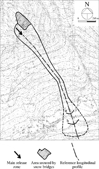
Fig. 2. Overview of the Solco avalanche site. The runout positions of more frequent events (a) and of the biggest known event for the site (b) are marked; the former refers to an avalanche event in January 1994 and was used for model calibration on this site.
Five meteorological stations located within the Valmalenco valley at altitudes from about 1000 to about 2100 m have been considered for analyzing the snow-precipitation regime pertaining to the considered site (Reference BarboliniBarbolini, 1999); the length of records of the different gauges varied from 5 to 29 years.
Application of the Monte Carlo procedure
The methods outlined above were used to derive site-specific probability distributions for HB Lr and μ for the Solco case-study; the details can be found in Reference BarboliniBarbolini (1999). In accordance with the Monte Carlo approach, 1000 values for each release variable (namely, HT and Lr) and 1000 values for the friction coefficient μ were randomly (and independently) generated from the related probability distributions, for both relatively frequent events (say T = 30 years) and extremely rare events (say T = 300 years); 1000 dynamical simulations were subsequently performed for each of the two cases. The friction coefficient n was set to a value n = 0.017 m s–1/2 (see Table 2), kept constant for all the simulations. The reference profile used for calculations is indicated in Figure 2.
In addition, two cycles of simulations considering the individual effects of uncertainties on the release condition and on the friction coefficient μ were carried out. Alternately, the friction parameter μ and the release variables HT and Lr were held constant at their mean value, while the other parameter was free to vary.
Results
Figure 3a-b display the results of simulations where the uncertainties underlying the definition of both the friction coefficient μ and the release conditions are simultaneously accounted for.
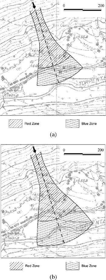
Fig. 3. Overview of the runout zone of the Solco site. For the cases T = 30years and T = 300years, average values and 95% confidence intervals for the runout distances (a) and for the final locations with 30 kPa impact pressure (b) are indicated along the reference profile (and expressed in meters measured along the path from the upper release point). The hatched rectangles have a length equal to one standard deviation. The dashed outline indicates the possible extension of the avalanche deposit, and has been determined from field surveys.
The obtained runout distances vary very strongly, both for relatively frequent events (up to 65 m) and for extremely rare events (up to 180 m). The variability of impact pressures, even if smaller, is still significant: the location of the 30 kPa impact pressure limit varies up to 40 m for relatively frequent events, and up to 120 m for extremely rare events. The degree of uncertainty of the results is strongly related to the considered return period: the confidence intervals for the case T = 300 years, for either runout distance or impact pressure, are about three times wider than those for the case T = 30 years. However, it is important to note that for this latter case the difference between the average runout distance and the downslope limits for the 95% confidence intervals would lead to the inclusion of both the main road and a group of houses in the zone endangered by the more frequent avalanches (Fig. 3a), with relevant consequences in terms of risk assessment for the considered area. Moreover, the mean values obtained for the runout distances, both for T = 30 years and for T = 300 years (Fig. 3a), are very close to the known extensions of relatively frequent and extreme historical events, respectively (Fig. 2). This appears to be an important confirmation of the effectiveness of the method introduced to define suitable friction coefficients for avalanche sites where the calibration data are limited or even completely lacking.
With respect to runout distance calculation, Figure 4a-b provide a comparison between the individual effects of the uncertainties in the release conditions and in the friction coefficient μ.

Fig. 4. Individual effects of the uncertainties of release conditions (lefthand side) and friction parameter μ (righthand side) on runout distance calculations. Average values and 95% confidence intervals are displayed along the reference profile. (a) T=30years; (b)T = 300 years.
For the case of relatively frequent events (Fig. 4a) the uncertainties in the friction coefficient μ and those in the release conditions have comparable effects on runout distance calculations. The respective 95% confidence intervals are very close, in terms of both location and width (about 35 m in both cases). The results for the case where both types of uncertainty are simultaneously accounted for (lefthand side of Fig. 3a) seem to combine the two separate effects, with the width of the 95% confidence intervals for runout distance (65 m) about twice that of the two previous cases. Conversely, for the case of extremely rare events (Fig. 4b) the uncertainties in the friction coefficient μ produce estimation errors of the runout distance that are considerably higher than those generated by the uncertainties in the initial conditions. The extension of the 95% confidence interval for the first case (160 m) is about twice that for the latter (75 m), and when combined (righthand side of Fig. 3a) only a small increase of the 95% confidence interval extension occurs with respect to that for the case of the friction coefficient μ only (righthand side of Fig. 4b). This result could have important practical consequences, if confirmed by further analysis made on other avalanche sites and using an enhanced module for the definition of the release variables (also able to account for uncertainties in the estimate of snowdrift overloads, for effects of release-area width variation, etc.). Provided the uncertainties in the release conditions for extreme avalanche events have negligible effects on runout distances relative to those for friction parameters, it would be possible to calibrate the model on the known extension of the deposits even where only a rough estimate of the release conditions is available, as is often the case for records of historical avalanches.
Concluding Remarks
The first practical implementation of the proposed method, without any claim for findings of general validity, supports its usefulness for reducing the overall degree of subjectivity in avalanche hazard assessments. Within the framework of a Monte Carlo approach there is no need to perform an arbitrary “a priori” definition of design conditions that can be thought to produce “safe enough” results. In fact, once the probability distributions for the various model outputs have been obtained, one can directly derive hazard maps with any desired level of reliability, simply by adopting the value with the appropriate non-exceedance probability P for each mapping variable (Fig. 5a and b).

Fig. 5. “Red/blue” hazard maps for given non-exceedance probabilities, (a) P = 0.5; (b) P = 0.975 The lower outlines of the hazard zones have been defined by circles drawn from the afex of the alluvial fan, with radius given by the runout position (and/or by the 30 kPa impact pressure location) calculated along the main flowline.
One important advantage of the proposed procedure is connected to its modular nature; the various simplifications currently introduced in each module do not in principle affect the validity of the overall approach, and might be removed once specific investigations and data collection have been carried out.
From a practical point of view, an immediate follow-up to the present work could reconsider the existing hazard maps by way of the proposed procedure, evaluating to what level of non-exceedance probability the current hazard limits actually conform. This analysis would present a valuable opportunity for standardizing the existing hazard cartography.
Acknowledgements
This research has been financially supported by the National Group for the Prevention of Hydrogeological Disasters (GNDCI) of the National Research Council of Italy (CNR). The authors gratefully acknowledge L. Natale for his guidance in the development of this work, and the Regional Snow and Avalanche Centres of Arabba and Bormio for key support of the data collection. Particular thanks go to C. Keylock for many helpful comments, to B. Sovilla for essential technical contributions and to D. Issler for stimulating discussions. M.B. gratefully acknowledges a research scholarship from the University of Pavia.


