


1. INTRODUCTION
Existing video coding standards, e.g. H.264/AVC [Reference Wiegand, Sullivan, Bjøntegaard and Luthra1], H.265/HEVC [Reference Sze, Budagavi and Sullivan2,Reference Sullivan, Ohm, Han and Wiegand3], or the currently developed versatile video coding (VVC) standard [Reference Bross, Chen and Liu4], exhibit coding artifacts due to block-based prediction and quantization [Reference Wiegand, Sullivan, Bjøntegaard and Luthra1–Reference Sullivan, Ohm, Han and Wiegand3]. These artifacts occur mainly through loss of high frequency details and manifest in discontinuities along block boundaries, error information near sharp transitions, or a smoothing of transitions, which correspond to blocking, ringing, or blurring artifacts. In order to reduce their visibility and therefore improve visual quality, in-loop filtering has emerged as a key tool. In the currently deployed HEVC video standard, two in-loop filters are included. The first one is the deblocking filter [Reference List, Joch, Lainema, Bjøntegaard and Karczewicz5–Reference Karimzadeh and Ramezanpour7]. Here, low-pass filters adaptively smooth boundary samples in order to suppress blocking artifacts. The second in-loop filter is the sample adaptive offset (SAO) [Reference Fu8] which tries to compensate for the sample distortion by classifying each sample into distinct classes with corresponding offset calculation for each class. The adaptive loop filter (ALF) [Reference Tsai9,Reference Karczewicz, Zhang, Chien and Li10] has been considered as a third in-loop filter after the deblocking filter and SAO for HEVC – see Fig. 1. It is currently discussed by the Joint Video Exploration Team (JVET) in the context of developing the new VVC standard. ALF has been adopted to the preliminary draft of VVC [Reference Bross, Chen and Liu4]. The main idea is to minimize the distortion between reconstructed and original samples by calculating Wiener filters at the encoder [Reference Slepian11,Reference Haykin12]. First, ALF applies a classification process. Each sample location is classified into one of 25 classes. Then for each class Wiener filters are calculated, followed by a filtering process.
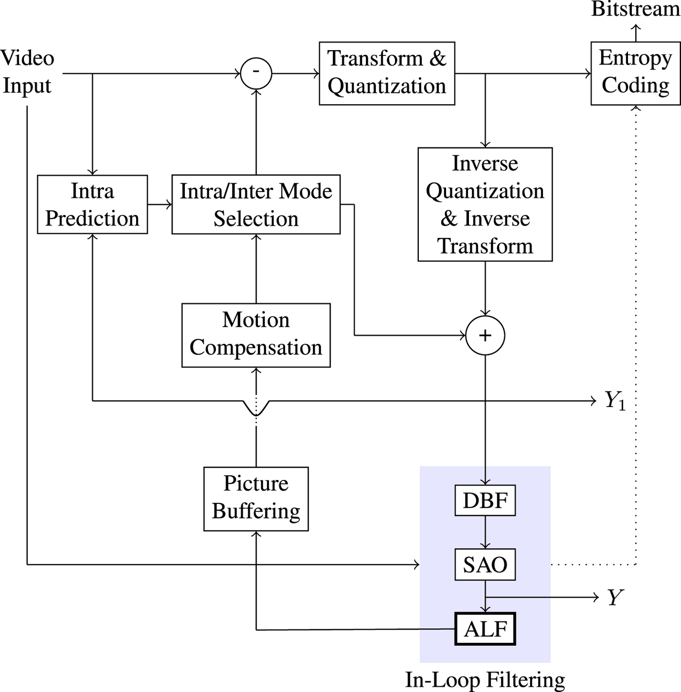
Fig. 1. Encoder block diagram: unfiltered and filtered images $Y_1$ and Y.
In the past few years, several novel in-loop filters have been investigated. Those are image prior models such as the low rank-based in-loop filter model which estimates the local noise distribution for coding noise removal [Reference Zhang13] and the adaptive clipping method where component-wise clipping bounds are calculated in order to reduce the error generated by the clipping process [Reference Galpin, Bordes and Racape14]. Others are convolutional neural network-based methods [Reference Jia15–Reference Kang, Kim and Lee20].
While the classification in ALF is derived mainly based on the local edge information, there are other underlying features such as textures. Therefore, instead of having a single classification, combining multiple classifications to incorporate various local image features simultaneously can lead to a better classification. This would improve the filtering process and eventually result in a higher coding efficiency.
Multiple classifications for ALF (MCALF) based on this approach have been recently introduced in [Reference Erfurt, Lim, Schwarz, Marpe and Wiegand21]. In this paper, we analyze MCALF and propose its extension to further improve coding efficiency. There are three main aspects of MCALF in this paper as follows. First, instead of having a single classification, applying multiple ones can lead to better adaptation to the local characteristics of the input image. Second, it would be natural to ask whether one can obtain an ideal classification for ALF. Such a classification is one which can classify all sample locations into the set of classes so that the filtering process provides the best approximation of the original image among all possible classifications. As this might be an infeasible task, we propose to approximate such an ideal classification with reasonable complexity. Finally, we extend the original MCALF by incorporating SAO nonlinear filtering. For this, we apply ALF with multiple classifications and SAO filtering simultaneously and introduce new block-based classifications for this approach.
The remainder of the paper is structured as follows. In Section 2, we briefly review the ALF algorithm currently part of the working draft of VVC [Reference Bross, Chen and Liu4]. In Sections 3 and 4, we review the original MCALF algorithm and propose several classifications for MCALF. Then in Section 5, we introduce our extended MCALF. In Section 6, simulation results are shown and we derive new block-based classifications. Finally, Section 7 concludes the paper.
2. REVIEW OF ALF
We review the main three procedures of ALF. These are the classification process, filter calculation, followed by the filtering process. For a complete description of ALF, we refer the reader to [Reference Tsai9] and [Reference Karczewicz, Zhang, Chien and Li10].
2.1. Laplace classification
A first step in ALF involves a classification $\mathcal {C}l$ . Each sample location $(i,j)$
 is classified into one of 25 classes $\mathcal {C}_1, \ldots ,\mathcal {C}_{25}$
 which are sets of sample locations. A block-based filter adaptation scheme is applied, all samples belonging to each $4\times 4$
 local image block share the same class index [Reference Karczewicz, Shlyakhov, Hu, Seregin and Chien22]. For this process, Laplacian and directional features are computed, involving calculation of gradients in four directions for the reconstructed luma samples – see Fig. 2.
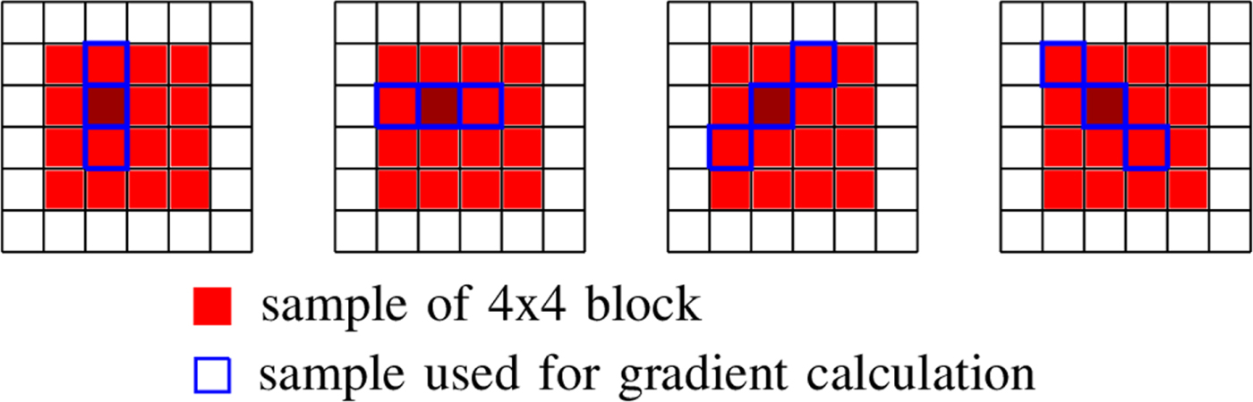
Fig. 2. Classification in ALF based on gradient calculations in vertical, horizontal, and diagonal directions.
Gradients for each sample location $(i,j)$ in four directions can be calculated as follows:

for the vertical and horizontal direction and

for the two diagonal directions, where Y is a reconstructed luma image after SAO is performed. First, for each $4\times 4$ block B, all of the gradients are calculated at the subsampled positions within a $8 \times 8$
 local block $\tilde B$
 containing B according to subsampling rule in [Reference Lim, Kang, Lee, Lee and Kim23]. The activity is then given as the sum of the vertical and horizontal gradients over $\tilde B$
 . This value is quantized to yield five activity values. Second, the dominant gradient direction within each block B is determined by comparing the directional gradients and additionally the direction strength is determined, which give five direction values. Both features together result in 25 classes. For the chroma channels no classification is performed.
2.2. Filter calculation
For each class $\mathcal {C}l$ , the corresponding Wiener filter $F_l$
 is estimated for $l\in \{1,\ldots ,25\}$
 by minimizing the mean square error (MSE) between the original image and the filtered reconstructed image associated with a class $\mathcal {C}l$
 . Therefore the following optimization problem has to be solved:

where X is the original image and ${\chi }_{\mathcal {C}_{\ell }}$ is the characteristic function defined by

To solve this optimization task in (1), a linear system of equations can be derived with its solution being the optimal filter $F_l$ . For a more detailed description of solving the optimization problem in (1), we refer the reader to [Reference Tsai9].
There is no classification applied for the chroma samples and therefore only one filter is calculated for each chroma channel.
2.3. Filtering process
Each Wiener filter $F_l\in \{1,\ldots ,{25}\}$ is obtained after solving the optimization problem in (1) for a given classification $\mathcal {C}l$
 and the resulting classes $\mathcal {C}_1,\ldots ,\mathcal {C}_{{25}}$
 . The filters $F_l$
 are symmetric and diamond-shaped – see Fig. 3. In VTM-4.0, they are $5\times 5$
 for chroma and $7\times 7$
 for the luma channel. They are applied to the reconstructed image Y resulting in a filtered image $X_{\mathcal {C}l}$
 as follows:

where L = 25 in this case. Figure 4 shows this filtering process.

Fig. 3. Symmetric diamond-shaped $7\times 7$ filter consisting of 13 distinct coefficients $c_0,\ldots ,c_{12}$
 .
.
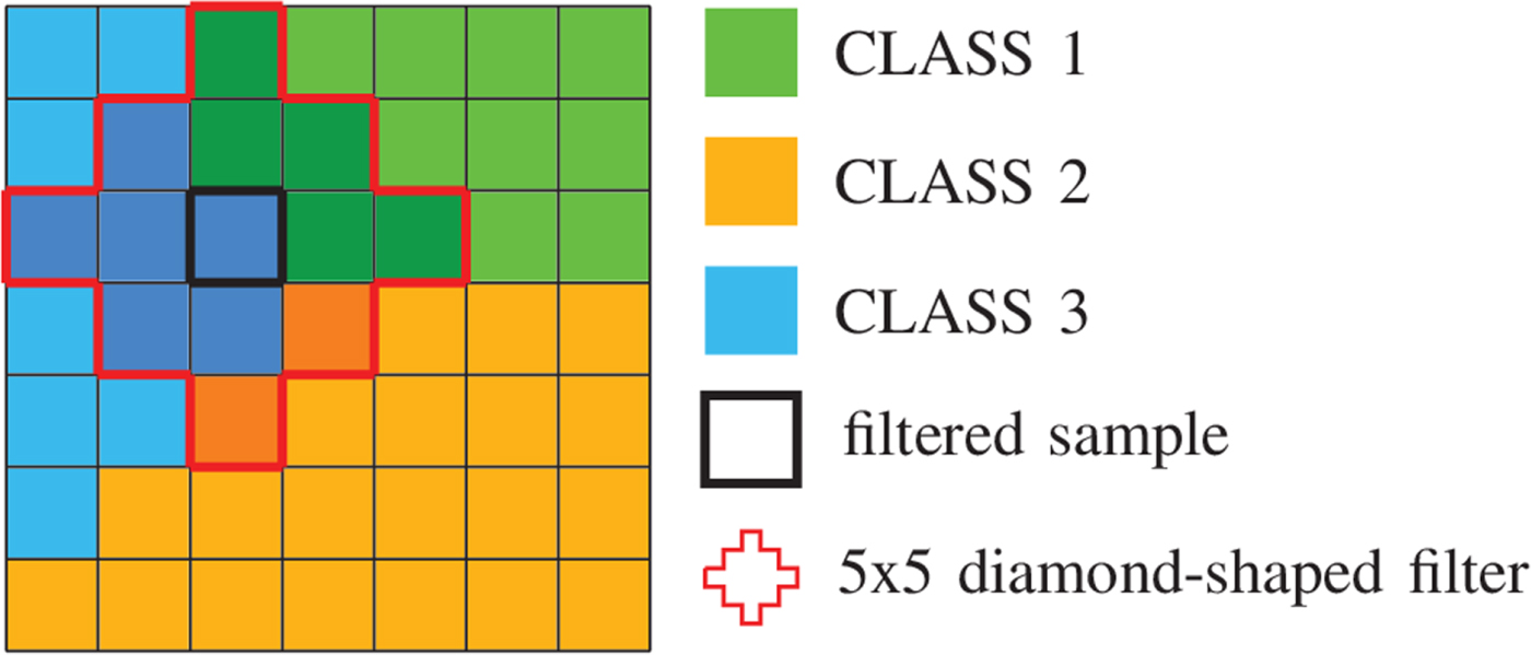
Fig. 4. Illustration of filtering process: each sample location is classified into one of three classes and filtered by a $5\times 5$ diamond-shaped filter. All shadowed samples affect the filtering process of the center location.
After the classification $\mathcal {C}l$ , a class merging algorithm is applied to find the best grouping of classes $\mathcal {C}_1,\ldots ,\mathcal {C}_{25}$
 by trying different versions of merging classes based onthe rate-distortion-optimizationprocess. This gives the merged classes $\tilde {\mathcal {C}}_1,\ldots ,\tilde {\mathcal {C}}_{\tilde L}$
 for some $\tilde L$
 with $1\leq \tilde L \leq 25$
 . In one extreme, all classes share one filter, when $\tilde L=1$
 ; in the other extreme, each class has its own filter, when $\tilde L=25$
 .
.
2.4. Other classification methods for ALF
In addition to Laplace classification, there are other classifications proposed during HEVC and its successor VVC standardization process. In [Reference Lai, Fernandes, Alshina and Kim24], subsampled Laplacian classification was proposed to reduce its computational complexity. Also, in [Reference Wang, Ma, Jia and Park25], the authors introduced a novel classification based on intra picture prediction mode and CU depth without calculation of direction and Laplacian features. Finally, a classification method incorporating multiple classifications has been proposed in [Reference Hsu26], which is similar to MCALF. We will provide some comparison test results for this approach in Section 6.
3. MULTIPLE FEATURE-BASED CLASSIFICATIONS
In this section, we describe various classifications for ALF. MCALF performs the same procedure as in ALF except for the modified classification process.
The main idea of MCALF is to take multiple feature-based classifications $\mathcal {C}l_1,\ldots ,\mathcal {C}l_M$ , instead of taking one specific classification as in ALF. Each classification $\mathcal {C}l_m$
 for $m\in \{1,\ldots ,M\}$
 provides a partition of the set of all sample locations of the currently processed frame and maps each sample location $(i,j)$
 to one of 25 classes $\mathcal {C}_1,\ldots ,\mathcal {C}_{25}$
 . The partition into 25 classes is obtained by

where I is the set of all sample locations in the input image. Then the corresponding Wiener filters $F_1,\dots ,F_{25}$ are applied to obtain the filtered reconstruction $X_{\mathcal {C}l_m}$
 in (3). Each classification among M choices results in a different reconstructed image and overhead that needs to be transmitted to the decoder. For evaluating the RD cost, $J_m$
 is calculated for each of M classifications $\mathcal {C}l_m$
 ,
,

where $D_m$ is a obtained distortion, $R_m$
 the rate depending on a classification $\mathcal {C}l_m$
 , and $\lambda \geq 0$
 the Lagrange multiplier. Note that different overhead impacts the RD cost. For instance, if the merging process after a classification with $\mathcal {C}l_{\tilde {m}}$
 , as described in Subsection 2-2.3, results in a larger number of Wiener filters than one with a classification $\mathcal {C}l_m$
 , it is very likely that $D_{\tilde {m}}$
 is smaller than $D_m$
 , while the rate $R_{\tilde {m}}$
 probably exceeds $R_m$
 . For a smaller number of filters after merging, one may expect that the corresponding distortion will be smaller and the rate larger. A classification with the smallest RD cost is chosen for the final classification, followed by the filtering process – see Fig. 5.

Fig. 5. MCALF at the encoder: filtering is performed after classifications $\mathcal {C}l_1,\ldots ,\mathcal {C}l_M$ carrying out (3). Classification with the smallest cost in (5) is chosen. After this RD decision, the corresponding classification and filtering are performed with the best RD-performance classification $\mathcal {C}l_\iota$
 .
.
3.1. Sample intensity based classification
The first classification $\mathcal {C}l_I$ is the simplest one and simply takes quantized sample values of the reconstructed luma image Y as follows:

where BD is the input bit depth and K the number of classes.
3.2. Ranking-based classification
The ranking-based classification $\mathcal {C}l_R$ ranks the sample of interest among its neighbors,

with l and h specifying the size of neighborhood. Note that when l=1 and h=1, $\mathcal {C}l_R$ is given as a map $\mathcal {C}l_R : I \rightarrow \{1,\ldots ,9\}$
 taking eight neighboring samples for $Y(i,j)$
 . In this case, $\mathcal {C}l_R(i,j)$
 simply ranks a sample value $Y(i,j)$
 in order of its magnitude compared to its neighboring samples. For instance, if $\mathcal {C}l_R(i,j)=1$
 , all neighboring sample locations of $(i,j)$
 have values greater than or equal to $Y(i,j)$
 . If $\mathcal {C}l_R(i,j)=9$
 then $Y(i,j)$
 has larger magnitude than its neighboring sample values. An example is shown in Fig. 6. Here, the center sample has five direct neighbors of smaller magnitudes and is therefore mapped to class index 6.
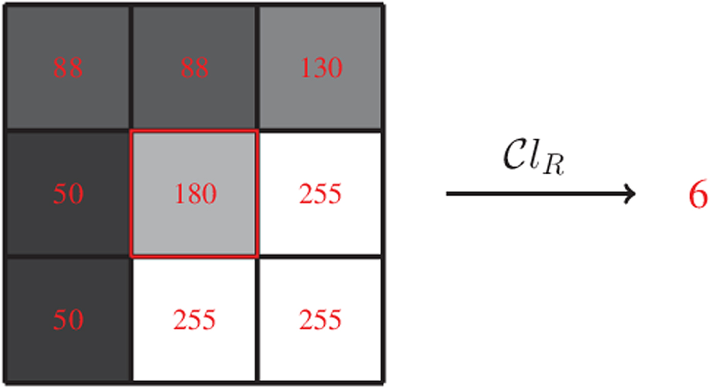
Fig. 6. Illustration of rank calculation of the center sample.
3.3. Classification with two features
Natural images are usually governed by more than one specific underlying local feature. To capture those features, we can apply a classification described by the product of two distinct classifications $\mathcal {C}l_1$ and $\mathcal {C}l_2$
 describing two distinct local features,

They can be joined together by a classification $\mathcal {C}l$ , which is the product of $\mathcal {C}l_1$
 and $\mathcal {C}l_2$
 ,
,

The constants $K_1$ and $K_2$
 define the number of classes $K = K_1 \cdot K_2$
 . When K exceeds the desired number of classes (for our experiments, we fix the number of classes for each classification as 25), $\mathcal {C}l(i,j)$
 can be quantized to have the intended number of classes $\bar {K}$
 . If $\mathcal {C}l(i,j)\in \{1,\ldots ,K\}$
 , then we apply a modified classification $\bar {\mathcal {C}l}$
 ,
,

The round-function maps the input value to the closest integer value. For instance, one can take $\mathcal {C}l_1 = \mathcal {C}l_I$ with $K_1=3$
 defined in (6) and $\mathcal {C}l_2 = \mathcal {C}l_R$
 as in (7) with l=1, h = 1 which gives $K_2=9$
 . The product of $\mathcal {C}l_I$
 and $\mathcal {C}l_R$
 results in $K=K_1\cdot K_2 = 27$
 classes. After quantization performed according to (9), we obtain $\bar {K} = 25$
 classes.
4. CLASSIFICATIONS WITH CONFIDENCE LEVEL
In the previous section, we proposed several classifications. A variety of classifications give the encoder more flexibility and it can choose the best one among the set of candidates. This is a rather quantitative approach of improving the state-of-the-art classification. As a second strategy, we propose a rather qualitative approach. Instead of proposing more classifications supporting different local features, we want to approximate an ideal classification.
4.1. Ideal classification
For fixed positive integers n and L, let $\mathcal {C}l^{id}$ be a classification with its corresponding classes $\mathcal {C}_1^{id},\ldots ,\mathcal {C}_L^{id}$
 and $n\times n$
 Wiener filters $F_1^{id},\ldots ,F_L^{id}$
 . Then, we call $\mathcal {C}l^{id}$
 an ideal classification if

for all possible classifications $\mathcal {C}l$ with the corresponding classes $\mathcal {C}_1, \ldots ,\mathcal {C}_L$
 and $n\times n$
 Wiener filters $F_1, \ldots ,F_L$
 . $X_{\mathcal {C}l^{id}}$
 and $X_{\mathcal {C}l}$
 are the filtered reconstructions according to (3). Equation (10) implies that an ideal classification leads to a reconstructed image $X_{\mathcal {C}l^{id}}$
 with the smallest MSE compared with X among all reconstructions $X_{\mathcal {C}l}$
 . Please note that this definition does not incorporate the merging process and the resulting rate. In fact, classes

with L = 2 were introduced for ideal classes in [Reference Erfurt, Lim, Schwarz, Marpe and Wiegand21]. In (11), I is the set of all luma sample locations and X and Y are original and reconstructed luma images respectively. Intuitively this partition into $\tilde {C}_1$ and $\tilde {C}_2$
 is reasonable. In fact, one can obtain a better approximation to X than Y by magnifying reconstructed samples $Y(i,j)$
 for $(i,j)$
 belonging to $\tilde {C}_1$
 and demagnifying samples associated with $\tilde {C}_2$
 . These samples have to be multiplied by a factor larger than 1 in the former and by a factor smaller than 1 in latter case.
4.2. Approximation of an ideal classification
To find a classification which gives a partition into the ideal classes $\tilde {\mathcal {C}}_1$ and $\tilde {\mathcal {C}}_2$
 might be an infeasible task. Instead, we want to approximate such a classification by utilizing information from the original image which need to be transmitted ultimately to the decoder.
Suppose we have a certain classification ${\rm {\cal C}}l:I\to \{ 1, \ldots ,9\} $ which can be applied for a reconstructed image Y at each sample location $(i,j) \in I$
 . Now, to approximate the two ideal classes $\tilde {\mathcal {C}}_1$
 and $\tilde {\mathcal {C}}_2$
 with $\mathcal {C}l$
 , we construct an estimate of those two classes, i.e. ${\mathcal {C}}^{e}_{1}$
 and ${\mathcal {C}}^{e}_{2}$
 as follows.
First, we apply a classification $\mathcal {C}l$ to pre-classify each sample location $(i,j)$
 into the pre-classes $\mathcal {C}_1^{pre}, \dots ,\mathcal {C}_9^{pre}$
 . For each $k \in \{1,\dots ,9\}$
 , $\mathcal {C}l(i,j) = k$
 implies a sample location $(i,j)$
 belongs to a class $\mathcal {C}_k^{pre}$
 . Now we measure how much accurately the classification $\mathcal {C}l$
 identifies sample locations in $\tilde {\mathcal {C}}_1$
 or $\tilde {\mathcal {C}}_2$
 . For this, we define $p_{k,1}$
 and $p_{k,2}$
 by
by

where $\vert A\vert$ is the number of elements contained in a set A. We call $p_{k,1}$
 and $p_{k,2}$
 confidence level. For a fixed positive constant $p \in (1/2,1)$
 and a given classification $\mathcal {C}l$
 , we now define a map $P_{\mathcal {C}l} : \{1,\ldots ,9\} \longrightarrow \{0,1,2\}$
 as follows:

The confidence level calculation is illustrated in Fig. 7. Here, a large part of $\mathcal {C}_k^{pre}$ intersect with the ideal class $\tilde {C}_2$
 , which leads to a high confidence level value $p_{k,2}$
 and ultimately sets $P_{\mathcal {C}l}(k) = 2$
 (if the constant p is reasonably high). We would like to point out that the map $P_{\mathcal {C}l}$
 can be given as a vector $P_{\mathcal {C}l} = (P_{\mathcal {C}l}(1), \ldots ,P_{\mathcal {C}l}(9))$
 of length 9 and one can now obtain $\mathcal {C}^e_{\ell }$
 by
by

using $P_{\mathcal {C}l}$ and $\mathcal {C}l$
 . Note that $\mathcal {C}^e_{\ell }$
 are obtained by collecting sample locations $(i,j)$
 which can be classified into the ideal classes $\tilde {\mathcal {C}}_{\ell }$
 with sufficiently high confidence (higher than p) by a given classification $\mathcal {C}l$
 . The vector $P_{\mathcal {C}l}$
 has to be encoded into the bitstream.
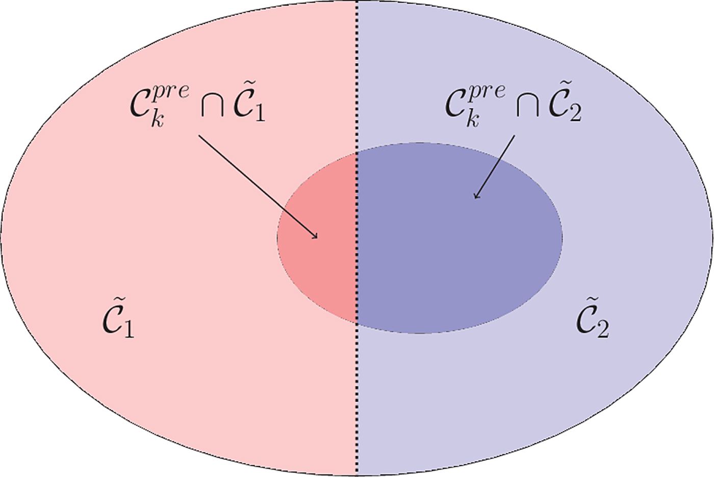
Fig. 7. Illustration of confidence level calculation. The outer ellipse is the set of all sample locations and divided into the ideal classes $\tilde {C}_1$ and $\tilde {C}_2$
 . The inner ellipse represents the pre-class $C_k^{pre}$
 for $k\in \{1,\ldots ,9\}$
 , which intersects with $\tilde {C}_1$
 and $\tilde {C}_2$
 .
.
Not all sample locations are classified by the classification $\mathcal {C}l$ into either $C_1^{e}$
 or $C_2^{e}$
 . Sample locations $(i,j)$
 with $P_{\mathcal {C}l}(\mathcal {C}l(i,j))=0$
 have to be classified with a second classification $\tilde {\mathcal {C}l}$
 , producing $\tilde {K}$
 additional classes,

This gives $\tilde {K}+2$ classes, namely $\mathcal {C}^e_{1}, \mathcal {C}^e_{2}, \mathcal {C}_1,\ldots ,\mathcal {C}_{\tilde {K}}$
 .
.
5. EXTENDED MCALF
The main drawback of a classification with the confidence level (13) to approximate the ideal classification (11) is that it requires extra coding cost for (13) and two classifications should be applied to construct classes $\mathcal {C}^e_{\ell }$ and $\mathcal {C}_{\ell }$
 in (14) and (15) which would increase computational complexity. To overcome this drawback, we first consider a classification first introduced in [Reference Lim, Schwarz, Marpe and Wiegand27], where it is used for SAO filtering. In fact, this approach allows for approximating the ideal classification (11) without computing the confidence level (13). Based on this, we then extend MCALF by incorporating additional SAO filtering.
We first note that the ideal classification in (11) is given by taking

The sign information in (16) cannot be obtained at the decoder since original sample $X(i,j)$ is not available. To approximate (16) without X, we first let $Y_1$
 be a reconstructed image before in-loop filtering is applied -- see Fig. 1. Then, we take $Y_1(i,j)-Y(i,j)$
 instead of $X(i,j)-Y(i,j)$
 . From this, we estimate the sign of $X(i,j) - Y(i,j)$
 by ${\rm sgn}(Y_1(i,j) - Y(i,j))$
 . Assume that

for some sufficiently large threshold T>0 so that

Then we have

Therefore, we can estimate the sign information $\mathcal {C}_{\rm {id}}(i,j)$ based on difference $D = Y_1 - Y$
 when (17) is satisfied with some relatively large T>0. From this, we now define

It should be noted that the estimate (18) would be more reliable for reconstructed samples $Y(i,j)$ satisfying (17) if we are allowed to increase T. In fact, some experimental results show $\mathcal {C}l_T$
 gives a better approximation for (11) for reconstructed samples satisfying (17) while the number of those samples decreases as we increase T. We refer the readers to [Reference Lim, Schwarz, Marpe and Wiegand27] for more details on this.
Next, we derive our extended MCALF using the classification $\mathcal {C}l_T$ we just described. Let $\mathcal {C}l$
 be a given classification providing K classes forming a partition of I. We also define

for $\ell = -1,0,1$ and
and

for $k = 1, \ldots ,K$ . For a fixed T>0, we now define a new in-loop filter using two classifications $\mathcal {C}l_T$
 and $\mathcal {C}l$
 as follows:

In (21), we extend (3) by combining filtering by Wiener filters $F_{k}$ associated with classes $\mathcal {C}_{k}$
 with SAO filtering by offset values $Q(d_{\ell })$
 with classes $\mathcal {D}_{\ell }$
 . The offset values $Q(d_{\ell })$
 are given as quantized values for $d_{\ell }$
 . Each $d_{\ell }$
 is chosen so that the MSE between the original image X and a reconstructed image by adding an offset value d to the sum of filtered images with $F_{k}$
 over $\mathcal {D}_{\ell }$
 is minimized with respect to d. This is given as

for $\ell = -1,0,1$ .
.
6. SIMULATION RESULTS AND ANALYSIS
In this section, we provide test results for two in-loop filtering algorithms based on our multiple classifications for ALF. We call those two methods MCALF-1, our original MCALF in [Reference Erfurt, Lim, Schwarz, Marpe and Wiegand21], and its extension MCALF-2 with a new reconstruction method (21) introduced in Section 5. We compare those two methods to the ALF algorithm based on VTM-4.0, the VVC test model (VTM) of version 4.0. VTM-4.0 is the reference software to the working draft 4 of the VVC standardization process [Reference Bross, Chen and Liu4,28]. Furthermore, we compare MCALF-2 to the ALF algorithm incorporating a different classification method in [Reference Hsu26].
6.1. Extension of original MCALF
The first algorithm MCALF-1 incorporates five classifications. For our extension MCALF-2, we apply a new reconstruction scheme (21) with three classifications consisting of Laplace classification and two additional classifications, which will be specified in the next section. We choose a threshold parameter T = 2 for $\mathcal {C}l_T$ to construct classes $\mathcal {D}_{\ell }$
 in (21). This parameter is experimentally chosen. Alternatively, it can be selected at the encoder so that the corresponding RD cost is minimized with this selected threshold. In this case, the selected threshold T should be transmitted to the bitstream.
6.2. Experimental setup
For the results of our experimental evaluation, we integrate our MCALF algorithms and compare VTM-4.0 + MCALF-1 and VTM-4.0 + MCALF-2 to VTM-4.0. Please note that ALF is adopted into the reference software. We also compare our MCALF approach to the ALF algorithm with the classification method in [Reference Hsu26]. In [Reference Hsu26], a classification method employing three classifications has been proposed. Two of the classifications are nearly identical to Laplace and sample intensity based classifications while the third one classifies samples based on similarity between neighboring samples. For this comparison test, we integrate those three classifications into VTM-4.0 and call it ALF-2.
The coding efficiency is measured in terms of bit-rate savings and is given in terms of Bjøntegaard delta (BD) rate [Reference Bjøntegaard29]. In the experiments, the total of 26 different video sequences, covering different resolutions including WQVGA, WVGA, 1080p, and 4K, are used. They build the set of sequences of the common test conditions (CTC) for VVC [Reference Boyce, Suehring, Li and Seregin30] The quantization parameterssettings are 22, 27, 32, and 37. The run-time complexity is measured by the ratio between the anchor and tested method.
6.2.1. MCALF-1
Five classifications are applied in MCALF-1 and all classifications provide a partition into K = 25 classes:
– Laplace classification which performs the classification process in ALF, explained in Section 2-2.1.
– Sample intensity based classification $\mathcal {C}l_I$
 .
.– Product of ranking-based and sample intensity based classifications $\mathcal {C}l_{R,I}$
with
(23)\begin{align} \mathcal{C}l_{R,I}(i,j) & = (\mathcal{C}l_R(i,j),\mathcal{C}l_I(i,j)) \nonumber \\ \quad &\in \{1,\ldots,9\}\times\{1,2,3\}. \end{align}$\mathcal {C}l_{R,I}(i,j)$ is quantized to one of 25 distinct values.– Classification with confidence level, using the classification $\mathcal {C}l_I$
to determine
\[ \mathcal{C}^e_{\ell} = \{(i,j) \in I : P_{\mathcal{C}l_I}(\mathcal{C}l_I(i,j)) = \ell\} \quad {\rm for}\ \ell = 1,2\]and Laplace classification for the remaining 23 classes. For this, instead of constructing 25 classes from Laplace classification, three classes with low activity values are put into one class, which gives 23 classes.
– Classification with confidence level, using $\mathcal {C}l_{R,I}$
to determine
\[ \mathcal{C}^e_{\ell} = \{(i,j) \in I : P_{\mathcal{C}l_{R,I}}(\mathcal{C}l_{R,I}(i,j)) = \ell\} \quad {\rm for}\ \ell = 1,2\]and Laplace classification for the remaining 23 classes as above.


6.2.2. MCALF-2
Laplace classification and two additional classifications are applied to construct $\mathcal {C}_k$ in (20). For the two additional classifications, we choose $\mathcal {C}l$
 in (20) as follows:
– Sample intensity based classification $\mathcal {C}l_I$
.– $\mathcal {C}l_{R,I}$
is quantized to one of 25 distinct values.


Both classifications provide 25 classes forming a partition of I. We then apply (21) with one of three classifications selected for $\mathcal {C}l$ in (20).
6.3. Evaluation of simulation results
Tables 1 and 2 show the results for random access (RA) and low delay B (LDB) configurations respectively. It is evident that RD performance is improved for both multiple classification algorithms MCALF-1 and MCALF-2. In particular, MCALF-2 algorithm increases coding efficiency up to $1.43\%$ for RA configuration. It should be also noted that MCALF-2 consistently outperforms MCALF-1 for all test video sequences except for one of screen content sequences, SlideEditing. The last three columns inTable 1 show how often each classification in MCALF-2 is selected for each test video sequence. This shows how each of classifications performs compared to others with respect to RD performance depending on test video sequences.
Table 1. Coding gains of MCALF-1 and MCALF-2 for RA configuration and percentage of each classification in MCALF-2.
Table 2. Coding gains of MCALF-1 and MCALF-2 for LDB configuration.
Furthermore, Tables 3 and 4 show the comparison results between ALF-2 and MCALF-2 for RA and LDB. It is clear that MCALF-2 consistently outperforms ALF-2 with the classification method in [Reference Hsu26] for all test video sequences.
Table 3. Coding gains of ALF-2 and MCALF-2 for RA configuration.
Table 4. Coding gains of ALF-2 and MCALF-2 for LDB configuration.
6.4. Discussion of complexity/implementation aspects
Having multiple classifications in general does not notably increase the complexity as each of classifications considered in this paper is comparable with Laplace classification in terms of complexity. For instance, the ranking-based classification $\mathcal {C}l_R(i,j)$ requires eight comparisons and eight additions for each $(i,j) \in I$
 . Therefore the total number of operations for $\mathcal {C}l_{R,I}$
 is comparable with Laplace classification with 176/16 additions and 64/16 comparisons for each sample location $(i,j) \in I$
 . We also note that $\mathcal {C}l_{I}$
 is less complex than $\mathcal {C}l_{R,I}$
 .
.
For Laplace classification, $4 \times 4$ block-based classification is recently adopted, which significantly reduces its complexity. One can also modify sample-based classifications $\mathcal {C}l_{I}$
 and $\mathcal {C}l_{R,I}$
 used in MCALF-2 so that resulting classifications are applied for each non-overlapping $4 \times 4$
 block. For this, we first define $4 \times 4$
 block $B(i,j)$
 for $(i,j) \in I$
 as follows:

For each block $B(i,j)$ , an average sample value over $B(i,j)$
 is given as

Then we define $4 \times 4$ block-based classifications for $\mathcal {C}l_{I}$
 and $\mathcal {C}l_{R,I}$
 by simply replacing $Y(i,j)$
 and $Y(k_1,k_2)$
 by $\overline {Y}(B(i,j))$
 and $\overline {Y}(B(k_1,k_2))$
 in (6) and (7). Finally, we apply (21) with those $4 \times 4$
 block-based classifications instead of $\mathcal {C}l_{R,I}$
 and $\mathcal {C}l_{I}$
 . This reduces its complexity compared to MCALF-2 and gives $-0.37 \%$
 (Y), $-0.86 \%$
 (U), $-0.74 \%$
 (V) coding gains on average for RA over 15 video sequences in classes A1, A2, B,and C.
There are two main issues for implementing MCALF-2. First, the classification $\mathcal {C}l_T$ in (18) requires extra memory to store a whole reconstructed image $Y_1$
 . One remedy for this would be to take the difference between two images Y and $\hat Y$
 , a reconstructed image obtained by applying filtering with Wiener filters $F_k$
 to Y, instead of $Y_1-Y$
 in (18). This approach can be then extended to take neighboring sample values of $Y(i,j)-\hat {Y}(i,j)$
 with some weights for $(i,j) \in I$
 as suggested in [Reference Lim, Schwarz, Marpe and Wiegand27], which can be further investigated for future work. Second, line buffer issue is always the key for any coding tool design. In particular, the size of the line buffer is determined by the vertical size of the filter employed in ALF. For this, one can further explore an approach [Reference Budagavi, Sze and Zhou31] to derive ALF filter sets with reduced vertical size.
7. CONCLUSION
In this paper, we studied multiple classification algorithms forALF and extended the original MCALF called MCALF-1 by applying adaptive loop filter and SAO filter simultaneously. Based on this, we developed a novel algorithm MCALF-2 and new block-based classifications. Both algorithms MCALF-1 and MCALF-2 were tested for RA and LDB configurations on the CTC data set consisting of 26 video sequences. It shows that MCALF-2 consistently outperforms MCALF-1 for all sequences except for one screen content sequence and a bit-rate reduction of more than 1% compared to the state-of-the-art ALF algorithm can be achieved.
Johannes Erfurt received his M.Sc. degree in mathematics from the Technical University of Berlin (TUB), Berlin, Germany, in 2015. His studies included an exchange withDurham University, UK as well as withTomsk Polytechnic University, Russia. In his master thesis, he studied concepts of sparse recovery for image and videos. He joined the Image and Video Coding Group of the Video Coding & Analytics Department at Fraunhofer Institute for Telecommunications, Heinrich Hertz Institute (HHI), Berlin, Germany in 2014 as a student. After university, he continued working at HHI as a Research Associate. His research interests include mathematical image and video processing, in-loop filtering, video quality assessment, and subjective coding.
Wang-Q Lim received his A.B. and Ph.D. degrees in mathematics fromWashington University, St. Louis, USA in 2003 and 2006, respectively. Before joining the Fraunhofer Heinrich Hertz Institute (HHI), he held postdoctoral positions at Lehigh University (2006--2008), the University of Osnabrück (2009--2011), and TU Berlin (2011--2015). He is one of the main contributors of shearlets, a multiscale framework which allows to efficiently encode anisotropic features in multivariate problem classes. Based on this approach, he has been working on various applications including image denoising, interpolation, inpainting, separation, and medical imaging. Currently, he is a research scientist in the Image and Video Coding group at the Fraunhofer Heinrich Hertz Institute and his research interests are mainly in applied harmonic analysis, image/video processing, compressed sensing, approximation theory, and numerical analysis.
Heiko Schwarz received his Dipl.-Ing. degree in electrical engineering and Dr.-Ing. degree, both from the University of Rostock, Germany, in 1996 and 2000, respectively. In 1999, Heiko Schwarz joined the Fraunhofer Heinrich Hertz Institute, Berlin, Germany. Since 2010, he is leading the research group Image and Video Coding at the Fraunhofer Heinrich Hertz Institute. In October 2017, he became Professor at the FU Berlin. Heiko Schwarz has actively participated in the standardization activities of the ITU-T Video Coding Experts Group (ITU-T SG16/Q.6-VCEG) and the ISO/IEC Moving Pictures Experts Group (ISO/IEC JTC 1/SC 29/WG 11-MPEG). He successfully contributed to the video coding standards ITU-T Rec. H.264 $\vert$ ISO/IEC 14496-10 (MPEG-4 AVC) and ITU-T Rec. H.265 $\vert$
 ISO/IEC 23008-2 (MPEG-H HEVC) and their extensions. Heiko Schwarz co-chaired various ad hoc groups of the standardization bodies. He was appointed as co-editor of ITU-T Rec. H.264 and ISO/IEC 14496-10 and as software coordinator for the SVC reference software. Heiko Schwarz served as reviewer for various international journals and international conferences. Since 2016, he is associate editor of the IEEE Transactions on Circuits and Systems for Video Technology.
Detlev Marpe received his Dipl.-Math. degree (with highest honors) from the Technical University of Berlin (TUB), Germany, and Dr.-Ing. degree in Computer Science fromthe University of Rostock, Germany. He is Head of the Video Coding & Analytics Department and Head of the Image & Video Coding Group at Fraunhofer HHI, Berlin. He is also active as a part-time lecturer at TUB. For nearly 20 years, he has successfully contributed to the standardization activities of ITU-T VCEG, ISO/IEC JPEG, and ISO/IEC MPEG in the area of still image and video coding. During the development of the H.264 $\vert$ MPEG-4 Advanced Video Coding (AVC) standard, he was chief architect of the CABAC entropy coding scheme as well as one of the main technical and editorial contributors to its Fidelity Range Extensions (FRExt) including the now ubiquitous High Profile. Marpe was also one of the key people in designing the basic architecture of Scalable Video Coding (SVC) and Multiview Video Coding (MVC) as algorithmic and syntactical extensions of H.264 $\vert$
 AVC. He also made successful contributions to the recent development of the H.265 $\vert$
 MPEG-H High Efficiency Video Coding (HEVC) standard, including its Range Extensions and 3D extensions. For his substantial contributions to the field of video coding, he received numerous awards, including a Nomination for the 2012 German Future Prize, the Karl Heinz Beckurts Award 2011, the 2009 Best Paper Award of the IEEE Circuits and Systems Society, the Joseph von Fraunhofer Prize 2004, and the Best Paper Award of the German Information Technology Society in 2004. As a co-editor and key contributor of the High Profile of H.264 $\vert$
 AVC as well as a member and key contributor of the Joint Collaborative Team on Video Coding for the development of H.265 $\vert$
 HEVC, he was corecipient of the 2008 and 2017 Primetime Emmy Engineering Award, respectively. Detlev Marpe is author or co-author of more than 200 publications in the area of video coding and signal processing, and he holds numerous internationally issued patents and patent applications in this field. His current citations are available at Google Scholar. He has been named a Fellow of IEEE, and he is a member of the DIN (German Institute for Standardization) and the Information Technology Society in the VDE (ITG). He also serves as an Associate Editor of the IEEE Transactions on Circuits and Systems for Video Technology. His current research interests include image and video coding, signal processing for communications as well as computer vision and information theory.
Thomas Wiegand is a professor in the department of Electrical Engineering and Computer Science at the Technical University of Berlin and is jointly leading the Fraunhofer Heinrich Hertz Institute, Berlin, Germany. He received his Dipl.-Ing. degree in Electrical Engineering from the Technical University of Hamburg-Harburg, Germany, in 1995 and Dr.-Ing. degree from the University of Erlangen-Nuremberg, Germany, in 2000. As a student, he was a Visiting Researcher at Kobe University, Japan, the University of California at Santa Barbara, and Stanford University, USA, where he also returned as a visiting professor. He was a consultant to Skyfire, Inc., Mountain View, CA, and is currently a consultant to Vidyo, Inc., Hackensack, NJ, USA. Since 1995, he has been an active participant in standardization for multimedia with many successful submissions to ITU-T and ISO/IEC. In 2000, he was appointed as the Associated Rapporteur of ITU-T VCEG and from 2005 to 2009, he was Co-Chair of ISO/IEC MPEG Video. The projects that he co-chaired for the development of the H.264/MPEG-AVC standard have been recognized by an ATAS Primetime Emmy Engineering Award. He was also a recipient of a ATAS Primetime Emmy Engineering Award for the development of H.265/MPEG-HEVC and a pair of NATAS Technology & Engineering Emmy Awards. For his research in video coding and transmission, he received numerous awards including the Vodafone Innovations Award, the EURASIP Group Technical Achievement Award, the Eduard Rhein Technology Award, the Karl Heinz Beckurts Award, the IEEE Masaru Ibuka Technical Field Award, and the IMTC Leadership Award. He received multiple best paper awards for his publications. Since 2014, Thomson Reuters named him in their list of ‘The World's Most Influential Scientific Minds’ as one of the most cited researchers in his field. He is a recipient of the ITU150 Award. He has been elected to the German National Academy of Engineering (Acatech) and the National Academy of Science (Leopoldina). Since 2018, he has been appointed the chair of the ITU/WHO Focus Group on Artificial Intelligence for Health.


 Open access