


1. INTRODUCTION
Glacier mass balance, as one of the most direct and reliable indicators of climate change, can quantitatively reveal whether there has been mass gain or loss in a glacier system (Bolch and others, Reference Bolch, Pieczonka and Benn2011; Gardelle and others, Reference Gardelle, Berthier, Arnaud and Kaab2013). Most of the previous studies have suggested that glaciers around the world have experienced obvious mass loss since the 1960s or 1970s (Berthier and others, Reference Berthier, Schiefer, Clarke, Menounos and Rémy2010; James and others, Reference James2012; Fischer and others, Reference Fischer, Huss and Hoelzle2015; Zhou and others, Reference Zhou, Li, Li, Zhao and Ding2018b), and that this condition was aggravated after the 1990s or 2000s, especially for high mountain regions in Asia (Bolch and others, Reference Bolch2012; Yao and others, Reference Yao2012; Gardner and others, Reference Gardner2013). Meltwater from glaciers in High Asia has not only contributed to a sea-level rise of 0.041 ± 0.009 mm a−1 for the period of 2000–16 (Brun and others, Reference Brun, Berthier, Wagnon, Kääb and Treichler2017), but, more importantly, it plays a crucial role in adjusting river runoff, while a proportion of the meltwater is temporarily stored in proglacial lakes (Gardelle and others, Reference Gardelle, Berthier, Arnaud and Kaab2013; Kääb and others, Reference Kääb, Treichler, Nuth and Berthier2015; Brun and others, Reference Brun, Berthier, Wagnon, Kääb and Treichler2017). In addition, drastic glacier changes can induce geological hazards (such as landslides, debris flows and glacier lake outburst floods), bringing potential security risks for downstream residents (Mergili and others, Reference Mergili, Müller and Schneider2013; Komatsu and Watanabe, Reference Komatsu and Watanabe2014; Lamsal and others, Reference Lamsal, Sawagaki, Watanabe and Byers2016). For the Pamir Mountains, in particular, which hold a considerable number of alpine glaciers, the question of how glaciers have changed in this region is significant and deserves to be of concern.
Over the entire Pamir, field-based measurements of mass balance (i.e. the glaciological method) have mainly concentrated on several small glaciers that are easy to reach, revealing a highly variable pattern of mass change in both space and time. For example, it has been reported that the Muztagh Ata Glacier in the eastern Pamir experienced a positive mass balance of 0.25 m w.e. a−1 for 2005–10 (Yao and others, Reference Yao2012), whereas the Abramov Glacier in the Pamir Alay showed significant mass loss at a rate of −0.46 ± 0.06 m w.e. a−1 for 1971–94 (Barandun and others, Reference Barandun2015). Since the field-based measurement technique is time-consuming and labor-intensive, it is not applicable to glacier change detection at a relatively large spatial scale, despite its advantage of high accuracy. As a complementary approach to investigate glacier mass balance, the geodetic method, which is primarily based on the differencing of multi-epoch topography products, has been widely and successfully used (Bolch and others, Reference Bolch, Buchroithner, Pieczonka and Kunert2008; Kääb and others, Reference Kääb, Berthier, Nuth, Gardelle and Arnaud2012, Reference Kääb, Treichler, Nuth and Berthier2015; Gardelle and others, Reference Gardelle, Berthier, Arnaud and Kaab2013; Li and others, Reference Li2017). Geodetic-based studies have suggested that the Pamir glaciers, as a whole, have generally been in a state of mass loss from 2000 to the mid-2010s (Table 1). For example, the use of ICESat laser altimetry products revealed a surface lowering of −0.13 ± 0.22 m a−1 for 2003–09 (Gardner and others, Reference Gardner2013) and −0.48 ± 0.14 m a−1 for 2003–08 (Kääb and others, Reference Kääb, Treichler, Nuth and Berthier2015). The discrepancy between these results is mainly due to the fact that the surface elevation of the Pamir glaciers is highly variable at the inter-annual scale (Brun and others, Reference Brun, Berthier, Wagnon, Kääb and Treichler2017). Based on the ASTER DEMs, updated results have suggested that there was only slight mass loss (−0.04 ± 0.07 m w.e. a−1) for 2000–16 (Brun and others, Reference Brun, Berthier, Wagnon, Kääb and Treichler2017). On a local scale, although a negative mass balance of −0.15 ± 0.12 m w.e. a−1 for 1971/76–2013/14 has been reported in the eastern Pamir (Zhang and others, Reference Zhang2016), most studies have suggested that the glaciers within this region have been in a balanced or positive state of mass budget from the 1970s to the mid-2010s (Table 1), e.g. −0.01 ± 0.30 m w.e. a−1 for 1973–2013 in Holzer and others (Reference Holzer2015) and 0.12 ± 0.07 m w.e. a−1 for 1999–2014 in Lin and others (Reference Lin, Li, Cuo, Hooper and Ye2017). The difference in the penetration depth correction of SRTM C-band radar largely accounts for the inconsistency of the existing results for the eastern Pamir (Table 1). In addition, over the central and western Pamir, previous studies mainly focusing on the changes since 2000 have reported seemingly divergent results for similar observation periods, e.g. 0.14 ± 0.14 m w.e. a−1 for 2000–11 (Gardelle and others, Reference Gardelle, Berthier, Arnaud and Kaab2013) versus −0.12 ± 0.06 m w.e. a−1 for 2000–14 (Lin and others, Reference Lin, Li, Cuo, Hooper and Ye2017). Nevertheless, according to the latest results of Brun and others (Reference Brun, Berthier, Wagnon, Kääb and Treichler2017) on a 1° × 1° geographic grid, it appears that the glaciers have likely been in a nearly stable state during 2000–16 in the central Pamir. Meanwhile, the western Pamir may have experienced a certain degree of mass wastage (see Fig. 2 in Brun and others (Reference Brun, Berthier, Wagnon, Kääb and Treichler2017) for details). In addition, especially for the Fedchenko Glacier situated in the central Pamir, long-term geodetic-based results have suggested that the glacier-wide mass balance has increased from −0.28 m w.e. a−1 for 1928–2000 (Lambrecht and others, Reference Lambrecht, Mayer, Aizen, Floricioiu and Surazakov2014) to −0.34 m w.e. a−1 for 2000–16 (Lambrecht and others, Reference Lambrecht, Mayer, Wendt, Floricioiu and Völksen2018).
Table 1. Summary of the existing region-wide glacier mass balances reported in the Pamir Mountains
From the above, clearly, there is a knowledge gap about how the central and western Pamir glaciers reacted to climate change before 2000. Hence, the key purpose of this study was to extend the timescale of investigating glacier mass balance in the central Pamir using the early KH-9 (Keyhole-9, also known as Hexagon) images, and to further promote the understanding of the glacier changes of this region for a longer time period.
2. STUDY AREA
Due to being affected by the prevailing westerlies, the Pamir Mountains in central Asia receive a large amount of precipitation at high elevations, and are one of the most important glacier centers in the mid- to low-latitudes (Chevallier and others, Reference Chevallier2014), covering a total area of ~12 000 km2 (excluding the Pamir Alay) (RGI Consortium, 2017). Most of the glaciers concentrate in the central Pamir, which has an area of ~5400 km2. The percentage of debris-covered glacier areas is ~8% in this region (Mölg and others, Reference Mölg, Bolch, Rastner, Strozzi and Paul2018). Of these glaciers, the Fedchenko Glacier, with a length of ~72 km and a total ice volume of ~124 km3, is one of the largest alpine glaciers in the world (Aizen and others, Reference Aizen2009; Lambrecht and others, Reference Lambrecht, Mayer, Aizen, Floricioiu and Surazakov2014). In addition, meteorological records from two observation stations (Gorbunov Station and Altynmazar Station, at altitudes of 4169 m and 2782 m a.s.l., respectively; Fig. 1a) reveal a considerable difference in the vertical distribution of the precipitation. At Altynmazar Station, the mean annual precipitation is 159 mm, which is only one-seventh of that at Gorbunov Station (~1140 mm). Most of the precipitation occurs in winter and spring (from December to May), with an average of ~890 mm (Gorbunov Station) and 113 mm (Altynmazar Station), accounting for 78 and 71% of the annual precipitation, respectively. This indicates that the central Pamir glaciers are of the winter-accumulation type (Maussion and others, Reference Maussion2014; Sakai and others, Reference Sakai2015). Moreover, the mean annual air temperature is −6.9 and 3.5 °C at Gorbunov Station and Altynmazar Station, respectively, indicating relatively cold climate conditions in this region. Furthermore, a typical characteristic for the central Pamir is that glacier surge behavior frequently occurs (Kotlyakov and others, Reference Kotlyakov, Osipova and Tsvetkov2008; Sevestre and Benn, Reference Sevestre and Benn2015; Wendt and others, Reference Wendt, Mayer, Lambrecht and Floricioiu2017), reflecting the instability of the glacier systems.
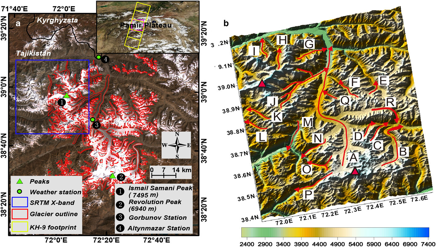
Fig. 1. (a) Mosaic true-color Landsat image for the central Pamir (24 August 2000 and 16 September 2000). (b) The topography of the study area (SRTM DEM) shown as a hillshade map. The red lines with arrows denote major glaciers and their flow directions. The capital letters from A to Q represent the glacier names. A − Fedchenko Glacier, B − Grum Grjimailo Glacier, C − Tanimas-2 Glacier, D − Tanimas-3 Glacier, E − N. Kyskurgan Glacier, F − Kosinenko Glacier, G − Little Tanimas Glacier, H − Ayujilga Glacier, I − Mushketov Glacier, J − Bivachny Glacier, K − Vavilov Glacier, L − Shokalski Glacier, M − RGS (Russian Geographical Society) Glacier, N − Bears Glacier, O − Abdukagor Glacier, P − Yazgulem Glacier, Q − Ulugbeka Glacier, R − N. Tanimas Glacier. Note that there are various groups of Tanimas Glaciers, five draining into the Tanimas River and one (N) on the eastern slope.
3 DATA PROCESSING
3.1 Glacier outlines
In this study, we did not generate our own glacier boundaries, but directly used the Randolph Glacier Inventory (RGI) Version 6.0 dataset, which was released on 28 July 2017 by the Global Land Ice Measurements from Space (GLIMS) initiative (http://www.glims.org/RGI/rgi60_dl.html). Considering that the Glacier Area Mapping for Discharge from the Asian Mountains (GAMDAM) inventory (with a mapping uncertainty of 15%, see Nuimura and others (Reference Nuimura2015)) is an important part of the RGI dataset, we assume that the uncertainty of the glacier outlines used in this study are at the order of 15%. In order to obtain the glacier extent that corresponds to the observation period of this study, the RGI v6.0 dataset was further modified by referring to two Landsat/ETM+ images (path/row: 151/033 and 152/033; date: 24 August 2000 and 16 September 2000) and ortho-rectified KH-9 images (acquired on 13 July 1975). The adjustments that we made included changes in the terminal positions of the glaciers due to glacier surge behavior and in lateral outlines because of surface thickening and thinning (King and others, Reference King, Quincey, Carrivick and Rowan2017). In addition, given the relatively low contrast of the KH-9 images, the final elevation difference map was used to help determine the glacier boundaries, especially for the debris-covered areas (Maurer and others, Reference Maurer, Rupper and Schaefer2016).
3.2 KH-9 DEM generation
The KH-9 images declassified by the US Geological Survey in 2002 record land surface information between 1971 and 1986 at a relatively fine scale (a spatial resolution of 6–9 m), and have become a very valuable data source for reconstructing historical topography (Surazakov and Aizen, Reference Surazakov and Aizen2010; Pieczonka and others, Reference Pieczonka, Bolch, Junfeng and Shiyin2013). In this study, we used the KH-9 triplet images to extract the KH-9 DEM via the Automated Terrain Extraction (ATE) routine contained in the ERDAS Leica Photogrammetry Suite (LPS) module. In the process of collecting the ground control points (GCPs), we used the Landsat/ETM+ images and the 1 arc-second SRTM DEM as the horizontal reference and the vertical reference, respectively (Pieczonka and others, Reference Pieczonka, Bolch, Junfeng and Shiyin2013; Zhou and others, Reference Zhou, Li and Li2017, Reference Zhou, Li, Li, Zhao and Ding2018b). A total of 43 GCPs were chosen at easily distinguished areas such as mountain ridges, river bends and road intersections. To independently examine the model error of the aerial triangulation, seven check points (CPs) were employed. Finally, the root-mean-square error (RMSE) of the stereo model was ~0.39 pixels, satisfying the constraint condition of being less than one pixel. The RMSEs of the GCP and CP residuals are ~10 m in the three directions (Table 2). For the extracted KH-9 DEM, statistics of the vertical accuracy with the GCPs and CPs as reference are given in Table 2. In addition, the DEM extraction report shows that most of the mass points (75.2%) used to interpolate the elevation in a regular grid are of good quality, with a correlation score above 0.7. The rest of the points (24.8%) have scores ranging from 0.5 to 0.7. Despite this, at high altitudes (e.g. in the accumulation zones), there are some clearly erroneous pixels characterized by irregular bulges in the hillshade map.
Table 2. The aerial triangulation information and vertical accuracy check for the generation of the KH-9 DEM
* The SD, MAE and RMSE, respectively, denote the std dev., mean absolute error and root-mean-square error.
3.3 DEM differencing and outlier elimination for the accumulation zones
As one of the most important topography data sources, the 1 arc-second SRTM C-band DEM taken in February 2000 was used as a reference in this study. Once the KH-9 DEM was produced, we followed the data processing strategy of Zhou and others (Reference Zhou, Li and Li2017, Reference Zhou, Li, Li, Zhao and Ding2018b) to check and correct some potential offsets and biases between the two DEMs. To be specific, we first co-registered the KH-9 DEM to the reference SRTM DEM using the classic method proposed by Nuth and Kääb (Reference Nuth and Kääb2011). Subsequently, we examined and corrected the tilt by fitting a second-order trend surface (Fig. S1), which is something that is often required for the DEMs derived from the early aerospace imagery (Bolch and others, Reference Bolch, Pieczonka and Benn2011, Reference Bolch, Pieczonka, Mukherjee and Shea2017; Pieczonka and others, Reference Pieczonka, Bolch, Junfeng and Shiyin2013; Li and others, Reference Li2017; Zhou and others, Reference Zhou, Li and Li2017, Reference Zhou, Li, Li, Zhao and Ding2018b). In addition, with regard to some potential biases associated with terrain parameters (e.g. elevation, slope, aspect and maximum curvature), we first checked the maximum curvature-dependent bias, given that it is likely to be the cause of the elevation-dependent bias (Paul, Reference Paul2008; Gardelle and others, Reference Gardelle, Berthier and Arnaud2012). We then examined the elevation-, slope- and aspect-dependent biases in sequence (Fig. S2). The residual elevation-dependent bias may result from an uneven spatial distribution of GCPs in the x-y-z planes (Nuth and Kääb, Reference Nuth and Kääb2011). The final elevation difference in the off-glacier areas is shown in Figure S3. The overall processing flow resulted in an improvement of the std dev. of the elevation difference in ice-free areas of 15.95% in total (Table 3).
Table 3. Statistics of the elevation differences in the ice-free areas for the raw and corrected difference maps
After performing the above corrections, similar to the findings of previous studies utilizing the KH-9 DEMs (Pieczonka and Bolch, Reference Pieczonka and Bolch2015; Maurer and others, Reference Maurer, Rupper and Schaefer2016; Bolch and others, Reference Bolch, Pieczonka, Mukherjee and Shea2017; Zhou and others, Reference Zhou, Li and Li2017, Reference Zhou, Li, Li, Zhao and Ding2018b), a remarkable surface lowering (more than 50 m) was found in the upper parts of the glacier accumulation zones (Fig. S4). Given that: (1) the KH-9 images have a relatively poor contrast in these snow-covered areas; and (2) the steep topography at high altitudes can easily induce the geometric distortion of stereo images, this phenomenon can be ascribed to erroneous matching of optical images in the process of producing the KH-9 DEM, and can thus be treated as outliers that need to be eliminated. In this study, with a prerequisite hypothesis that glacier thinning gradually decreases with the increase in altitude following a non-linear trend (Schwitter and Raymond, Reference Schwitter and Raymond1993), we applied the simple and effective method proposed by Zhou and others (Reference Zhou, Li, Li, Zhao and Ding2018b), who adopted a quadratic function to approximately reflect the non-linear variation. To be more specific, the first step was to normalize the elevation in the glacier areas (Eqn (1)), and the next step was to determine a proper range (Δh range) of glacier elevation changes by adjusting an empirical coefficient (A) (Eqn (2)).
 $$\gamma = \displaystyle{{E_{\max} -E_{\rm g}} \over {E_{\max} -E_{\min}}}, $$
 $$\Delta h_{{\rm range}} = A\gamma ^2,$$
where E max,E min and E g represent the maximum elevation, the minimum elevation and the elevation at a given point in the glacier areas. γ is the normalizing factor. It should be noted that the setting of the empirical coefficient primarily depends on the performance of the outlier removal in the accumulation zones. After many trials, the coefficient was specified as −190, which results in the elevation changes in the upper part of the accumulation zones being limited to the range of ±10 m after the outlier elimination. However, this also causes somewhat excessive elimination for effective elevation changes in local ablation zones, especially for the surge-type glaciers. We filled these gaps using the original values. The final elevation difference map after removing the outliers is shown in Figure S4, where the proportion of the data gaps reaches 42%.
3.4 Radar penetration correction
Previous studies have shown that the penetration depth of C-band radar has become one of the most significant uncertainty sources when comparing SRTM C-band DEMs with other topography data obtained by optical or laser sensors (Gardelle and others, Reference Gardelle, Berthier, Arnaud and Kaab2013; Kääb and others, Reference Kääb, Treichler, Nuth and Berthier2015). In this study region, based upon the differencing operation between the SRTM C-band DEM and the X-band DEM, Gardelle and others (Reference Gardelle, Berthier, Arnaud and Kaab2013) and Lin and others (Reference Lin, Li, Cuo, Hooper and Ye2017) have reported an average penetration depth difference of 1.80 and 1.88 m, respectively. In this study, given that the penetration depth mainly depends on the physical characteristics of the glacier surface (Rignot and others, Reference Rignot, Echelmeyer and Krabill2001), in order to better elaborate the penetration depth difference for different glacier surfaces, we used the Landsat-7 image acquired on 16 September 2000 (close to the end of the ablation season) to separate the debris-covered areas, bare ice and firn/snow-covered areas based on the band ratio method. To be specific, the ratio of band 3 (red channel) to band 5 (mid-infrared channel) with a threshold of 2 was used to distinguish the ice and snow from debris-covered areas. We further applied a single-band thresholding approach (band 3: digital number>165) to identify the perennial snow-covered areas. After producing the classification map of glacier surfaces, we generated the mean penetration depth difference of each 100 m altitude interval for every category and performed the correction for each class using an overall average. It should be noted that we eliminated some pixels where the terrain slopes were >30°, in order to avoid introducing elevation bias induced by the steep topography. Moreover, prior to computing the penetration depth difference for the glacier areas, a mean residual (0.67 m) in the ice-free areas, possibly reflecting a systematic vertical offset, was subtracted.
In addition, given that: (1) the X-band radar can penetrate the glacier surface (mainly referring to the dry snow layer) to as deep as 3–6 m (Dehecq and others, Reference Dehecq, Millan, Berthier, Gourmelen and Trouve2016; Zhao and Floricioiu, Reference Zhao and Floricioiu2017); and (2) Wendt and others (Reference Wendt, Mayer, Lambrecht and Floricioiu2017) and Lambrecht and others (Reference Lambrecht, Mayer, Wendt, Floricioiu and Völksen2018) found a maximum penetration depth of the X-band radar of ~6 m (with an average of 3–4 m) (TanDEM-X data) in the upper part of the Fedchenko Glacier's accumulation zones, there is no doubt that the C-band radar penetration depth we obtained is underestimated. Nevertheless, considering that this region generally receives a large amount of winter snowfall that is dry and cold, especially at high altitudes, the SRTM X-band DEM likely represents the glacier surface elevation at the end of the ablation season in 1999. This also means that the glacier surface elevation in summer of 1999 can be approximately recovered by performing the correction of the penetration depth difference for the SRTM C-band DEM. In others words, the impact on the final mass balance of the C-band radar absolute penetration depth being underestimated may not be significant, as the KH-9 images were only acquired in summer. Based on this, we assume that the seasonal change caused by the difference of the data acquisition times (mid-July versus mid-February) is negligible, given the long observation period.
3.5 Mass-balance calculation
To calculate the glacier mass balance, we first generated the histogram of the glacier elevation change with elevation bins of 100 m. Due to the large number of data gaps caused by outlier elimination at high altitudes, in order to obtain the volume change of the whole glacier area, we assigned the average elevation change to these voids in a given elevation band. The volume change was then converted to the mass change using a factor of 0.85 ± 0.06 (Huss, Reference Huss2013). For each surge-type glacier, the mass balance was separately calculated. In addition, given that the difference in the strategies of filling data voids may lead to discrepant results, we calculated the mass balance for individual glaciers by replacing these holes with zeros based on the above method. To further test the influence of different settings of the empirical coefficient (see Section 3.2) on the mass-balance results, we used a simple approach of directly calculating the average mass balance for the entire region when the coefficient was specified as −130, −160, −190, −220 and −250, respectively.
3.6 Uncertainty evaluation
With regard to the accuracy assessment of the glacier mass balance, we used the std dev. (σ z) of the elevation differences for each elevation band (i) in stable regions to represent the uncertainty of the glacier elevation change of each pixel (Gardelle and others, Reference Gardelle, Berthier, Arnaud and Kaab2013). When calculating the average elevation change for a given elevation band, we needed to consider the influence of spatial autocorrelation between DEMs for the sake of evaluating the uncertainty (E z) (Eqn (3)) (Rolstad and others, Reference Rolstad, Haug and Denby2009). Based on the elevation difference map over the off-glacier areas, we fitted an experimental anisotropic semi-variogram using a spherical model (Fig. S5), and obtained a spatial autocorrelation distance (D) of 720 m (Eqn (4)).
 $$E_{{\rm z},i} = \displaystyle{{\sigma _{{\rm z},i}} \over {\sqrt {N_{{\rm eff},i}}}}, $$
 $$N_{{\rm eff},i} = \displaystyle{{N_{{\rm t},i}R} \over {2D}},$$
where N t, N eff and R represent the total number of observations, the number of independent measurements and the spatial resolution (30 m). Subsequently, the volume change uncertainty for a given glacier or region (E v) was calculated by Eqn (5).
 $$E_{\rm v} = \sqrt {\sum {{(E_{{\rm z},i}S_i)}^2}}, $$
where S denotes the glacier area in a given altitude interval. To further calculate the uncertainty of the mass balance, with an assumption of a 15% glacier area error (E S) (Nuimura and others, Reference Nuimura2015) and an uncertainty for the conversion factor of 0.6 ( $E_{{\rm f}_{\rm c}}$), the initial mass-balance uncertainty ( $E_{{\rm b}\_0}$) can be obtained by Eqn (6) based on the standard error propagation law.
 $$E_{{\rm b}\_0} = \sqrt {{\left( {\displaystyle{V \over {S_{\rm t}}}\cdot E_{{\rm f}_{\rm c}}} \right)}^2 + {\left( {\displaystyle{{\,f_{\rm c}} \over {S_{\rm t}}}\cdot E_{\rm V}} \right)}^2 + {\left( {\displaystyle{{V\cdot f_{\rm c}} \over {S_{\rm t}^2}} \cdot E_{\rm s}} \right)}^2}, $$
where V and S t denote the volume change and the total glacier area for a glacier or region. f c is the conversion factor (0.85). In addition, since the penetration depth correction has a systematic effect on the final mass change, the uncertainty of the mass balance can thus be further expressed as  $E_{{\rm b}\_1}$ (Eqn (7)).
 $$E_{{\rm b}\_1} = \sqrt {E_{{\rm b}\_0}^2 + E_{{\rm b}\_{\rm p}}^2}, $$
where  $E_{{\rm b}\_{\rm p}}$ represents the uncertainty of the penetration correction, which was set to 1.28 m w.e. in this study (assuming a penetration depth error of 1.5 m) (Gardelle and others, Reference Gardelle, Berthier, Arnaud and Kaab2013). Moreover, to further account for the uncertainty caused by the data gaps and the outlier elimination, we introduced a scale factor (1/(1 − R void)) and an additional factor ( $E_{{\rm b}\_{\rm c}}$) to calculate the final mass-balance uncertainty (E b) by using Eqn (8).
 $$E_{\rm b} = \displaystyle{2 \over {1-R_{{\rm void}}}}\cdot E_{{\rm b}\_1} + E_{{\rm b}\_{\rm c}},$$
where R void denotes the proportion of the data gaps (Table 4). It should be pointed out that the scale factor was conservatively multiplied by 2, given that almost half the pixels were removed, which likely led to larger uncertainty for the glacier mass change. In particular, for the uncertainty induced by the setting of the empirical coefficient, we chose the maximum range of the change of the mass-balance results in different scenarios as the additional factor (0.06 m w.e. a−1 in the present study).
Table 4. The average elevation change and the mass balance for individual glaciers and the whole region between 1975 and 1999. Method 1: assuming zero change for missing data. Method 2: using average elevation changes at the same altitude bands to fill the gaps. Note that this study uses the results obtained by Method 2
* The SLE represents the snow line elevation, which was obtained by reference to the Landsat images (16 September 2000) and the SRTM DEM.
† denotes the surge-type glaciers. Note that the SG1–3 glaciers were used in this study to represent three unnamed glaciers.
4. RESULTS
4.1 Penetration depth difference
The final results show that the average penetration depth difference is 0.06 m for debris-covered areas (accounting for 18.5% of the selected areas), 1.68 m for bare ice areas (46.6%) and 2.96 m for firn/snow-covered areas (34.9%). In particular, based on a visual analysis of the available optical images, we speculated that the 0.06 m residual in the debris-covered areas is possibly caused by wet snow, as there was heavy snowfall in this area before 5 February 2000 (not shown), and most of the snow remained on 13 February 2000 (Fig. 2). Hence, we did not take this term into account for the correction. The penetration difference estimate we obtained is close to that of Holzer and others (Reference Holzer2015) in the bare ice areas (i.e. 1.68 versus 1.50 ± 0.90 m), but is lower than that in the firn/snow areas (2.96 versus 4.30 ± 0.90 m). The latter represents the average of the penetration depth estimation over three regions (Karakoram, Hindu Kush and Jammu Kashmir), which were calculated by extrapolating the ICESat trend to the moment of SRTM acquisition, theoretically reflecting an absolute penetration depth. In addition, our penetration depth difference results are more or less higher than the estimates of Zhang and others (Reference Zhang2016) for different glacier surfaces in the eastern Pamir (i.e. 0.79 and 2.41 m for the bare ice and the firn/snow covered areas, respectively) (Table 1). This can be attributed to the regional difference in glacier characteristics. Finally, the area-weighted average penetration depth difference is 1.82 m for the whole region, which is in line with the existing estimates in Gardelle and others (Reference Gardelle, Berthier, Arnaud and Kaab2013) and Lin and others (Reference Lin, Li, Cuo, Hooper and Ye2017). In contrast, over the entire Pamir, Kääb and others (Reference Kääb, Treichler, Nuth and Berthier2015) found an average penetration depth of 5–6 m, which may be overestimated. This is because ICESat data samples are relatively sparse in the Pamir, and frequent glacier surges probably induce elevation bias, as stated by Kääb and others (Reference Kääb, Treichler, Nuth and Berthier2015). The updated glacier mass balance by Brun and others (Reference Brun, Berthier, Wagnon, Kääb and Treichler2017) (−0.04 ± 0.19 m w.e. a−1 for 2000–08) indicates that the results of Kääb and others (Reference Kääb, Treichler, Nuth and Berthier2015) (−0.41 ± 0.12 m w.e. a−1 for 2003–08) may be biased; thus, obtaining the penetration depth from ICESat data is problematic.
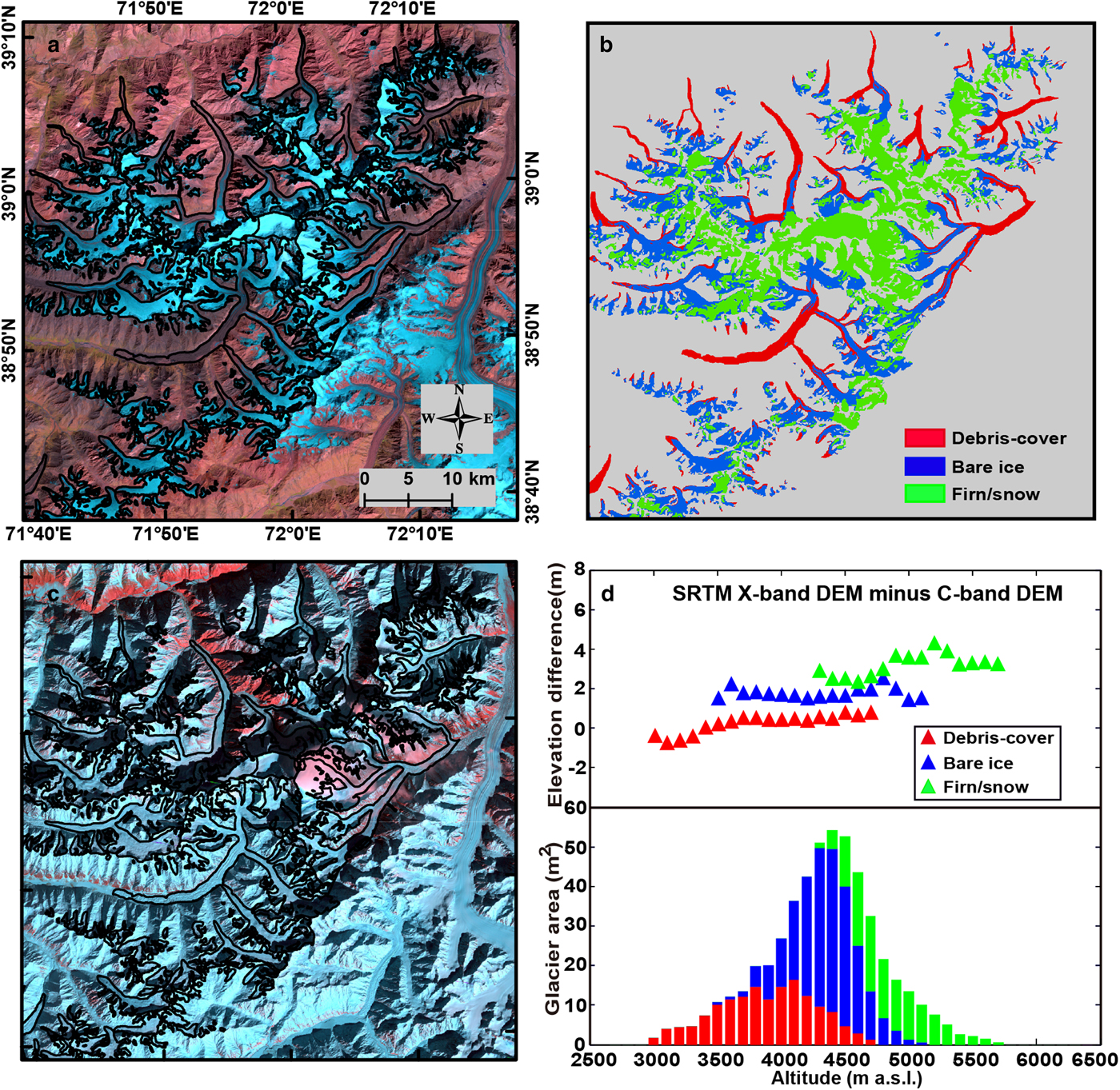
Fig. 2. (a) The Landsat false-color image (RGB: bands 5/4/3) acquired on 16 September 2000. (b) The classification map of the glacier surface. (c) The Landsat false-color image (RGB: bands 5/4/3) on 13 February 2000. (d) The area-altitude distribution and the penetration depth difference for each category.
4.2 Glacier elevation change
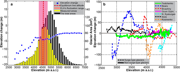
From Figure 3, we can clearly see that some glaciers experienced significant surface thickening and thinning in their lower and upper parts, respectively (e.g. Bivachny Glacier, Kosinenko Glacier, Vavilov Glacier, Shokalski Glacier, Yazgulem Glacier and Bears Glacier), implying the emergence of surging in our observation period. In particular, at the forefront of the Bears Glacier, a striking thinning of ~−130 m can be observed (Fig. 4b). Such a pattern can be ascribed to two catastrophic surge events that occurred in 1973 and 1989, respectively. The magnitude of the earlier surge was greater than that of the later (Harrison and others, Reference Harrison, Haeberli, Whiteman and Shroder2015), resulting in continuous thinning at the advanced fronts after 1973. A similar condition emerges at the terminus of the Kosinenko Glacier. In contrast, for the N. Kyskurgan Glacier, its accumulation and ablation zones, respectively, showed significant thickening and thinning (i.e. 0.50 ± 0.31 and −1.87 ± 0.31 m a−1 on average) (Table 4; Fig. 4b). This pattern indicates that the glacier surged before 1975 and was in a post-surge or quiescent phase for this study period. Similar conditions can be found on the nearby glaciers and the N. Tanimas Glacier. On the RGS Glacier, the ablation zone as a whole exhibited a moderate thickening (~10–15 m). This may have been caused by a micro-surge at the beginning of the 1970s (Kotlyakov and others, Reference Kotlyakov, Osipova and Tsvetkov2008). Moreover, according to previous studies, there are four additional small surge-type glaciers in this region (i.e. Ravak Glacier and the SG1–3 glaciers in Fig. 3) (Kotlyakov and others, Reference Kotlyakov, Osipova and Tsvetkov2008; Gardelle and others, Reference Gardelle, Berthier, Arnaud and Kaab2013). Although from the elevation change pattern only the Ravak Glacier clearly exhibits the surge features (Fig. 3), the statistical results suggested that the others may also have experienced micro-surges (Table 4). For the non-surge-type glaciers, the most representative Fedchenko Glacier showed an average thinning of −0.33 ± 0.33 m a−1 in the ablation zone and a near-zero change (0.02 ± 0.33 m a−1) in the accumulation zone (Table 4; Fig. 4b). Detailed information of the remaining glaciers is given in Table 4.
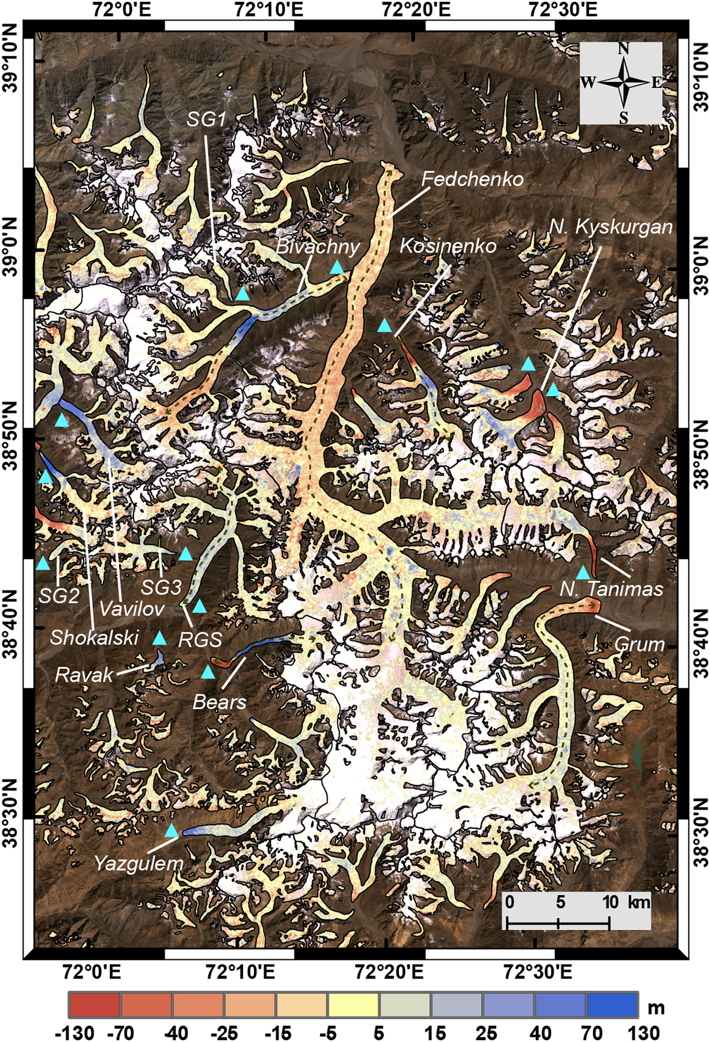
Fig. 3. Glacier elevation changes in the central Pamir for 1975–2000. The purple dotted lines represent the profiles in Figure 4b along the central flowline. The black lines denote the glacier boundaries. The cyan triangles represent the surge-type glaciers. The background is the Landsat true-color images, and the white areas (not covered by the elevation change map) represent the extent of the data gaps.

Fig. 4. (a) The area-elevation distribution and average elevation change with a 100 m elevation interval for all of the non-surge-type glaciers. (b) The elevation changes of some representative glaciers along the central flowline.
4.3 Glacier mass balance
With regard to the mass change, from 1975 to 1999, the central Pamir glaciers (covering a total glacier area of 2020.3 km2), as a whole, showed a nearly balanced or slightly negative mass balance of −0.03 ± 0.24 m w.e. a−1, which is equivalent to a mass deficit of −0.06 ± 0.48 Gt a−1. Of these glaciers, the Tanimas-3 Glacier and N. Kyskurgan Glacier showed the most negative mass balance, with a value of −0.12 ± 0.26 m w.e. a−1, while the most significant mass gain, at a rate of 0.63 ± 0.20 m w.e. a−1, occurred at the Ravak Glacier. For the Fedchenko Glacier, the mass balance was −0.09 ± 0.28 m w.e. a−1, corresponding to a mass wastage of −0.05 ± 0.15 Gt a−1. The mass change results for the other glaciers are listed in Table 4. In addition, for the surge-type glaciers (468.9 km2) and non-surge-type glaciers (1651.4 km2), their mass balances were 0.03 ± 0.14 and−0.05 ± 0.28 m w.e. a−1, respectively.
4.4 Sensitivity to outlier elimination and data gap filling
With regard to the outlier elimination for the accumulation zones, when the empirical coefficient was set as −130, −160, −190, −220 and −250, the corresponding region-wide mean mass balance was −0.01, −0.02, −0.04, −0.05 and −0.07 m w.e. a−1, respectively. The maximum difference between these results is 0.06 m w.e. a−1, which is within the error bars. In addition, the estimate of −0.04 m w.e. a−1 calculated based on the average of the whole area agrees with that (−0.03 m w.e. a−1) obtained by the different calculation approach with respect to the surge-type glaciers. For the processing of the data gaps, the two results based on the different gap-filling strategies are basically consistent (Table 4). The region-wide mass balance (filled with zeros) was −0.01 ± 0.24 m w.e. a−1, and the non-surge-type and surge-type glaciers showed a mass balance of −0.02 ± 0.28 and 0.03 ± 0.14 m w.e. a−1, respectively. For individual glaciers, the differences between these two results are generally <0.03 m w.e. a−1, but reach as high as 0.06 m w.e. a−1 for the Kosinenko Glacier and N. Tanimas Glacier. Even so, all the differences are within the error bars, suggesting good compatibility.
5. DISCUSSION
5.1 Comparison with previous studies
For the Fedchenko Glacier, Lambrecht and others (Reference Lambrecht, Mayer, Aizen, Floricioiu and Surazakov2014) reported an ice loss of −4.1 km3 (equivalent to a mass budget of −0.39 m w.e. a−1) for 1958–2000 in its main trunk. This is more negative than our estimate of −0.20 m w.e. a−1 for 1975–99 in similar areas. Similarly, in its ablation zone, volume change rates for each 100 m elevation band in this study are smaller than theirs on the whole (Fig. 5), but the variation trends are basically consistent, particularly in areas below 3800 m elevation. This seems to suggest a relatively high rate of mass loss in the lower part of the Fedchenko Glacier between 1958 and 1975. Nevertheless, there is no other evidence to support this intuitive speculation due to the lack of both in situ measurements and remote-sensing data for that period. Above an elevation of 3800 m, the two rates are almost equal in areas between 3800 and 4300 m, and exhibit a greater fluctuation above 4300 m. This local variation may be caused by inaccurate matching in the course of generating the KH-9 DEM and/or the ‘terracing’ effect within the earlier DEM (for 1958) obtained by interpolating from the topographic maps (Racoviteanu and others, Reference Racoviteanu, Manley, Arnaud and Williams2007). Other reason for the above discrepancies is the difference in the observation periods. Detailed comparison results are given in Table S1. Furthermore, in comparison with the glacier-wide results after 2000 (e.g. −0.27 ± 0.05 m w.e. a−1 for 2000–11 and −0.51 ± 0.06 m w.e. a−1 for 2011–16) reported by Lambrecht and others (Reference Lambrecht, Mayer, Wendt, Floricioiu and Völksen2018), this study period experienced less mass loss (−0.20 m w.e. a−1). The findings reveal an intensified mass wastage at the Fedchenko Glacier, especially after 2011, as reported in Lambrecht and others (Reference Lambrecht, Mayer, Wendt, Floricioiu and Völksen2018).
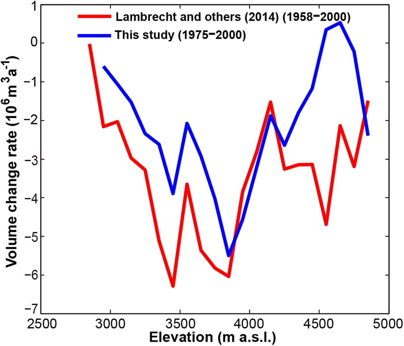
Fig. 5. Comparison of the mean volume change rate (for each altitude interval of 100 m) in the Fedchenko Glacier's ablation zone (with an altitude range of 2800–4850 m) between Lambrecht and others (Reference Lambrecht, Mayer, Aizen, Floricioiu and Surazakov2014) and this study.
As for the region-wide glacier mass change, it is important to note that we did not make a comparison of our geodetic results (in local regions) before 2000 with those of the entire Pamir after 2000, given the spatio-temporal heterogeneity of the glacier change pattern within this area. For the central Pamir, our estimate of −0.03 ± 0.24 m w.e. a−1 lies in between two previous results (i.e. 0.14 ± 0.14 in Gardelle and others (Reference Gardelle, Berthier, Arnaud and Kaab2013) and −0.12 ± 0.06 m w.e. a−1 in Lin and others (Reference Lin, Li, Cuo, Hooper and Ye2017)), but is closer to the result of Lin and others (Reference Lin, Li, Cuo, Hooper and Ye2017), despite a substantial overlap of error bounds. However, considering the pattern of glacier elevation change from Brun and others (Reference Brun, Berthier, Wagnon, Kääb and Treichler2017) (not affected by the radar penetration depth), we can deduce that the central Pamir glaciers have most likely been in an approximately balanced state over the past four decades (from the mid-1970s to the mid-2010s). Moreover, by comparing the mass changes of the surge-type and non-surge-type glaciers (i.e. 0.19 ± 0.22 and 0.12 ± 0.11 m w.e. a−1, respectively), Gardelle and others (Reference Gardelle, Berthier, Arnaud and Kaab2013) concluded that the surge behavior did not significantly affect the region-wide mass balance over a short time period (~10 years). This agrees with our findings prior to 2000, with a change of 0.03 ± 0.14 (surge-type) and −0.05 ± 0.28 m w.e. a−1 (non-surge-type). Coincidentally, in two observation periods (1975–99 and 2000–11), the differences between these two results are very close, i.e. 0.07 m w.e. a−1 in Gardelle and others (Reference Gardelle, Berthier, Arnaud and Kaab2013) and 0.08 m w.e. a−1 in this study. From the above, it appears that the conclusion of Gardelle and others (Reference Gardelle, Berthier, Arnaud and Kaab2013), i.e. the surge behavior did not significantly affect the region-wide mass balance, is valid for a longer period, at least from our observation results.
5.2 Potential reasons for the glacier changes
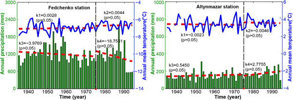
In order to understand the causes of the glacier mass changes in the central Pamir, we used the meteorological records for 1935–94 from Gorbunov Station and Altynmazar Station (Williams and Konovalov, Reference Williams and Konovalov2008). The relevant data have been subjected to rigorous quality checks (e.g. correcting the precipitation bias for the gauge type) and homogeneity adjustment (only for the precipitation data). More details can be found in the user guide (http://nsidc.org/data/G02174). In this study, we analyzed the variation trends of annual precipitation and mean air temperature for two sub-periods (1935–75 and 1975–94), as shown in Figure 6. Overall, it seems that both precipitation and temperature at high altitudes (i.e. Gorbunov Station) show an opposite tendency compared with low altitudes (Altynmazar Station) within the two sub-periods. For the period 1975–94, the low altitudes show signs of increased precipitation and decreased temperature, whereas there is rising temperature and decreased precipitation at high altitudes, especially for 1990–94. Moreover, it should be stated that the mean annual air temperature at low altitudes showed an increasing trend for the whole period, and the magnitude of the warming (k = 0.0041, p > 0.05) appears to have been lower than that (k = 0.0085, p > 0.05) at high altitudes. From the above, we intuitively speculate that the rising air temperature and decreased total precipitation at high altitudes to a great extent account for the slight mass loss, despite the increased precipitation and decreased temperature at low altitudes.
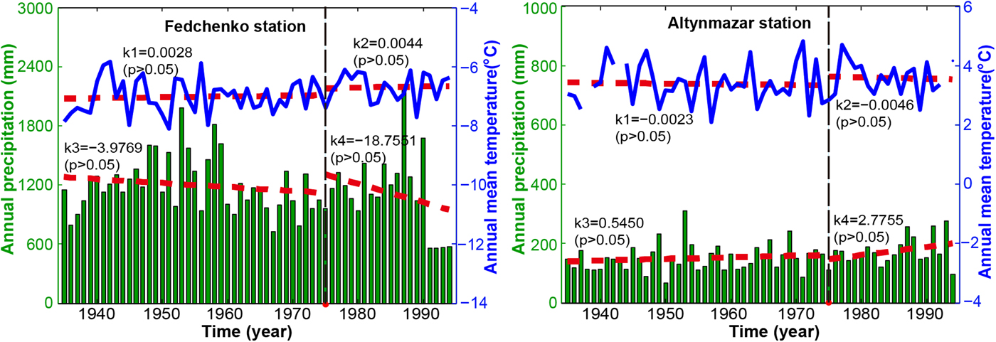
Fig. 6. Mean annual air temperature and precipitation for 1935–94. The red dashed line represents the regressed linear trend, and ‘k’ and ‘p’ denote the slope of the regressed trend and the significance level.
In addition, on a larger spatial scale, Zhou and others (Reference Zhou, Aizen and Aizen2018a) generated a unified air temperature and precipitation dataset (including a gap-filled station dataset and a derived grid dataset) for 1951–2010 by compiling and merging meteorological observation materials from 457 stations in central Asia. Analyzing the datasets suggests that central Asia, overall, experienced statistically significant warming around the 1970s, while the mean annual precipitation did not show prominent change over the whole period (Zhou and others, Reference Zhou, Aizen and Aizen2018a). This, to some extent, supports the above speculation.
6. CONCLUSIONS
Based on the early KH-9 stereo images and the 1 arc-second C-band SRTM DEM, this study evaluated the glacier mass change for 1975–99 in the central Pamir by employing the approach of DEM differencing. To alleviate the impact of the C-band radar penetrating into the glacier surface, we separately estimated the penetration depth differences for different glacier facies by subtracting the SRTM C-band DEM from the X-band DEM. The obtained penetration corrections were zero for debris-covered areas, 1.68 m for clean ice and 2.96 m for firn/snow areas. Finally, the overall mass balance was found to be −0.03 ± 0.24 m w.e. a−1 for 1975–99, indicating a nearly balanced state or very slight mass wastage. This may be attributed to the decreased precipitation and increased air temperature at high altitudes. Individual glaciers have shown a highly heterogeneous pattern of mass change, due to the glacier surge activity, with the mass balance varying from −0.12 ± 0.26 to 0.63 ± 0.20 m w.e. a−1. For the largest Fedchenko Glacier, it showed a negative mass balance of −0.09 ± 0.28 m w.e. a−1, corresponding to a mass budget of −0.05 ± 0.15 Gt a−1. In addition, for the different types of glacier (surge and non-surge), the mean mass balances were 0.03 ± 0.14 and −0.05 ± 0.28 m w.e. a−1, respectively. Given the natural defects of the KH-9 images and the uncertainty sources caused by the data processing, we tested the effect of outlier elimination and data gap filling on the final mass balance. The results suggest that our findings are quite robust for the chosen geodetic method, given the large uncertainty range. Finally, integrating our results with those of previous studies indicates that, over the past four decades (between the mid-1970s and the mid-2010s): (1) the central Pamir glaciers have been in a nearly stable state or have shown only slight mass loss; (2) the collective geodetic mass balance of glaciers that surged during the study period was similar to that of glaciers that did not surge.
SUPPLEMENTARY MATERIAL
The supplementary material for this article can be found at https://doi.org/10.1017/jog.2019.8
ACKNOWLEDGEMENTS
We thank the US Geological Survey for providing the Landsat images, the KH-9 images and the SRTM C-band DEM data. We also thank the German Aerospace Center (DLR) for providing the SRTM X-band DEM and the National Snow and Ice Data Center for providing the meteorological data. The glacier inventory (RGI, v6.0) was provided by the GLIMS initiative. We also thank all of the editors and reviewers for their constructive comments, which greatly improved the quality of this paper. We also acknowledge the support of Dr Hang Zhou of the University of Idaho. The work in this paper was supported by the National Natural Science Foundation of China (grant Nos. 41474007, 41574005) and the Independent Exploration and Innovation Funds of Central South University (grant No. 2017zzts173).


 Open access