


1. Introduction
The equation of state (EOS) of carbon at high pressures is a subject of interest for several branches of science, including astrophysics, material science, and applied engineering (first of all including fusion research). In particular, a very important point (in particular for the explanation of large magnetic fields of giant planets such as Uranus and Neptune) is the existence of a metallic phase of carbon[Reference Bundy1–Reference Correa, Bonev and Galli4]. To reach it in laboratory conditions, it is possible to use laser-driven shocks. The pressure (in Mbar) of such shocks can be estimated by  $P= 11. 6\mathop{(I/ 1{0}^{14} )}\nolimits ^{3/ 4} {\lambda }^{- 1/ 4} \mathop{(A/ 2Z)}\nolimits ^{7/ 16} \mathop{({Z}^{\ast } t/ 3. 5)}\nolimits ^{- 1/ 8} $, where $I$ is the laser intensity on the target in $\mathrm{W} / {\mathrm{cm} }^{2} , \lambda $ is the laser wavelength in $\unicode[.5,0][STIXGeneral,Times]{x03BC} \mathrm{m} $, and $A, Z$, and ${Z}^{\ast } $, respectively, are the mass number, the atomic number, and the effective ionization degree of the target, and the time $t$ is in ns[Reference Batani, Balducci, Nazarov, Lower, Hall, Koenig, Faral, Benuzzi and Temporal5]. So intensities of the order of $1{0}^{14} ~\mathrm{W} / {\mathrm{cm} }^{2} $, which can be obtained quite easily, allow getting pressures of the order of 10 Mbar.
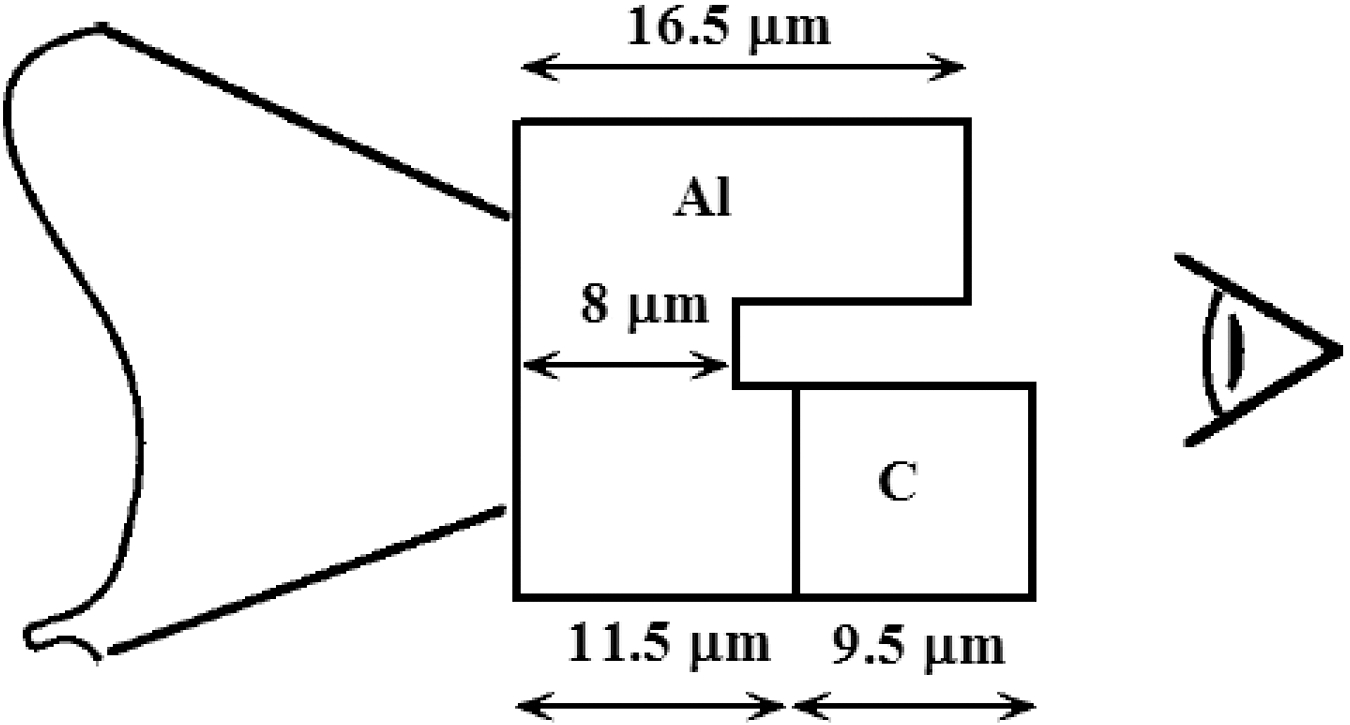
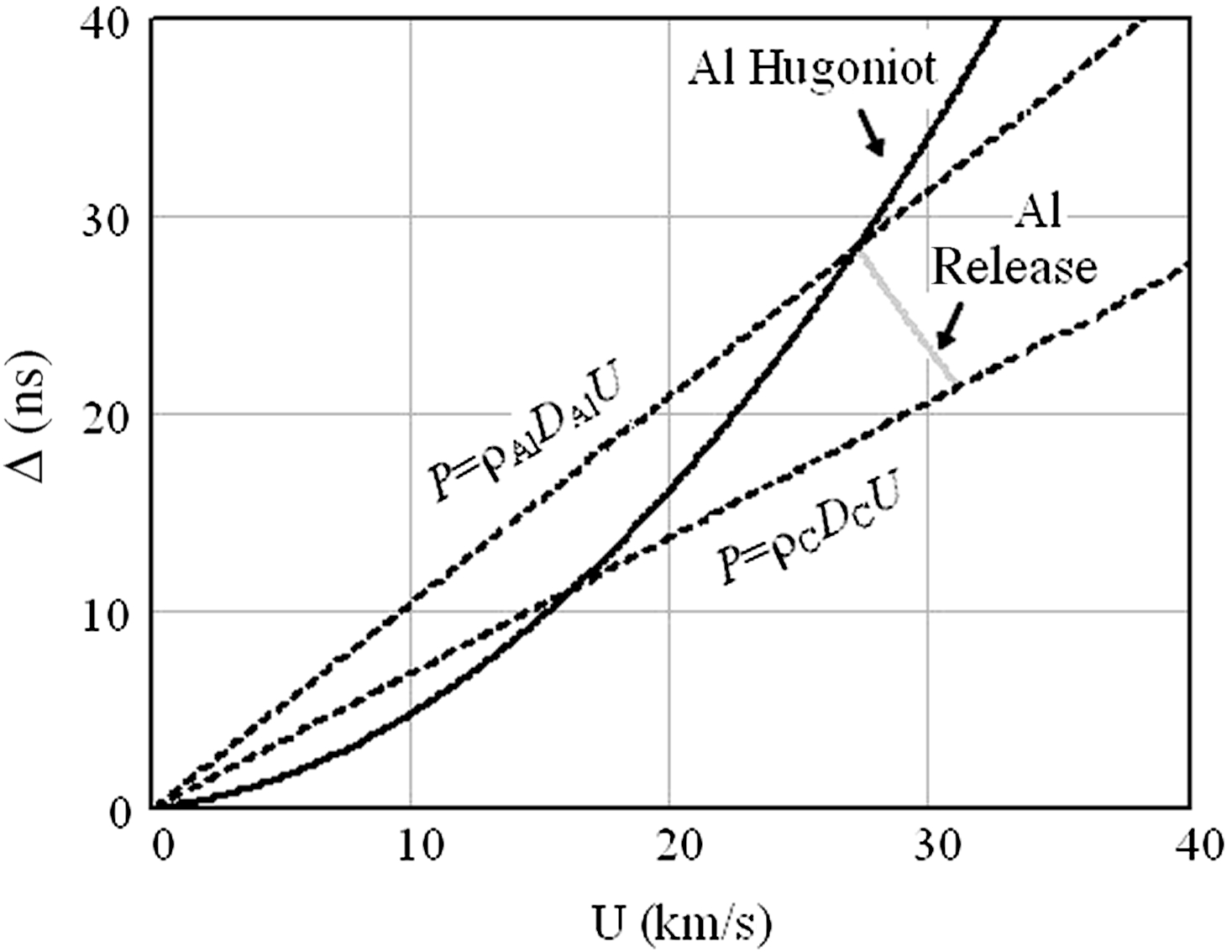
A well-known experimental method to measure the EOS is based on the impedance mismatch technique and consists in measuring the shock velocity of two different materials (test and reference) at the same time. The shock-wave measurements are realized by a streak camera recording the emission from the rear side of the shocked target. Using time-resolved imaging, we can experimentally determine the times of the shock arrival for each part of target (see Figure 1), and afterwards the velocity of the shock propagating through the two steps,  ${D}_{\mathrm{Al} } $ and ${D}_{\mathrm{C} } $. Then if the EOS (and hence the shock adiabat) of the base material (aluminium) is known, we can calculate an EOS point for the test material (carbon) as the intersection in the ( $P, U$) plane of the line $P= {\rho }_{\mathrm{C} } {D}_{\mathrm{C} } U$ (momentum conservation law; ${\rho }_{\mathrm{C} } $ is the density of cold carbon) with the reflected isentropic release drawn from the intersection of $P= {\rho }_{\mathrm{Al} } {D}_{\mathrm{Al} } U$ ( ${\rho }_{\mathrm{Al} } $ is the density of cold aluminium) with the aluminium Hugoniot adiabat (see Figure 2)[Reference Zel’dovich and Raizer6,Reference Celliers, Collins, Hicks and Eggert7] .
One of the critical points of this method is the effect of the temporal profile of the high-power pulse. Indeed, an ideal shock can be produced only with a high-power flat-top laser pulse, and the analysis of the effect of the real temporal profile of a high-power laser in experiments is important, because it can be a substantial contribution to the total experimental error. The aim of the present work was to realize a set of simulations for Gaussian pulses with different durations and to analyse the effect on the calculation of shock velocities.

Figure 1. Sketch of the configuration of EOS measurements using the impedance mismatch technique. A streak camera measures the times of the shock arrival; the shock velocities  ${D}_{\mathrm{Al} } $ and ${D}_{\mathrm{C} } $ are calculated from the difference of these times.
Figure 2. Calculation of the  $(P, U)$ EOS point for carbon from measured ${D}_{\mathrm{Al} } , {D}_{\mathrm{C} } $ and Al Hugoniot adiabat using the impedance mismatch method.
2. Simulations
For the realization of simulations we have used the hydrocode MULTI (multigroup radiation transport in multilayer foils)[Reference Ramis, Schmalz and Meyer-ter-Vehn8]. We have used the SESAME equation of state for aluminium[Reference Holian9] and porous carbon EOS calculated by MPQEOS[Reference Kemp and Meyer-ter-Vehn10] with a reduced initial density ( $1. 6~\mathrm{g} / {\mathrm{cm} }^{3} $)[Reference Aliverdiev, Batani, Dezulian and Vinci11,Reference Aliverdiev, Batani, Dezulian and Vinci12] , as presented in Ref. Ref. [Reference Batani, Strati, Stabile, Tomasini, Lucchini, Ravasio, Koenig, Benuzzi-Mounaix, Nishimura, Ochi, Ullschmied, Skala, Kralikova, Pfeifer, Kadlec, Mocek, Prag, Hall, Milani, Barborini and Piseri13]. For each case we have realized three different 1D ‘sub-simulations’ for the three parts of the target: (i) $\mathrm{Al} ~8~\unicode[.5,0][STIXGeneral,Times]{x03BC} \mathrm{m} $, (ii) $\mathrm{Al} ~16. 5~\unicode[.5,0][STIXGeneral,Times]{x03BC} \mathrm{m} $, and (iii) $Al{\unicode{x2013}}C ~11. 5~\unicode[.5,0][STIXGeneral,Times]{x03BC} \mathrm{m} + 9. 5~\unicode[.5,0][STIXGeneral,Times]{x03BC} \mathrm{m} $ corresponding to Al base, Al step, and carbon step (see Figure 1), and have determined the shock arrival times to the rear target surface, as in the real experiment[Reference Batani, Strati, Stabile, Tomasini, Lucchini, Ravasio, Koenig, Benuzzi-Mounaix, Nishimura, Ochi, Ullschmied, Skala, Kralikova, Pfeifer, Kadlec, Mocek, Prag, Hall, Milani, Barborini and Piseri13].
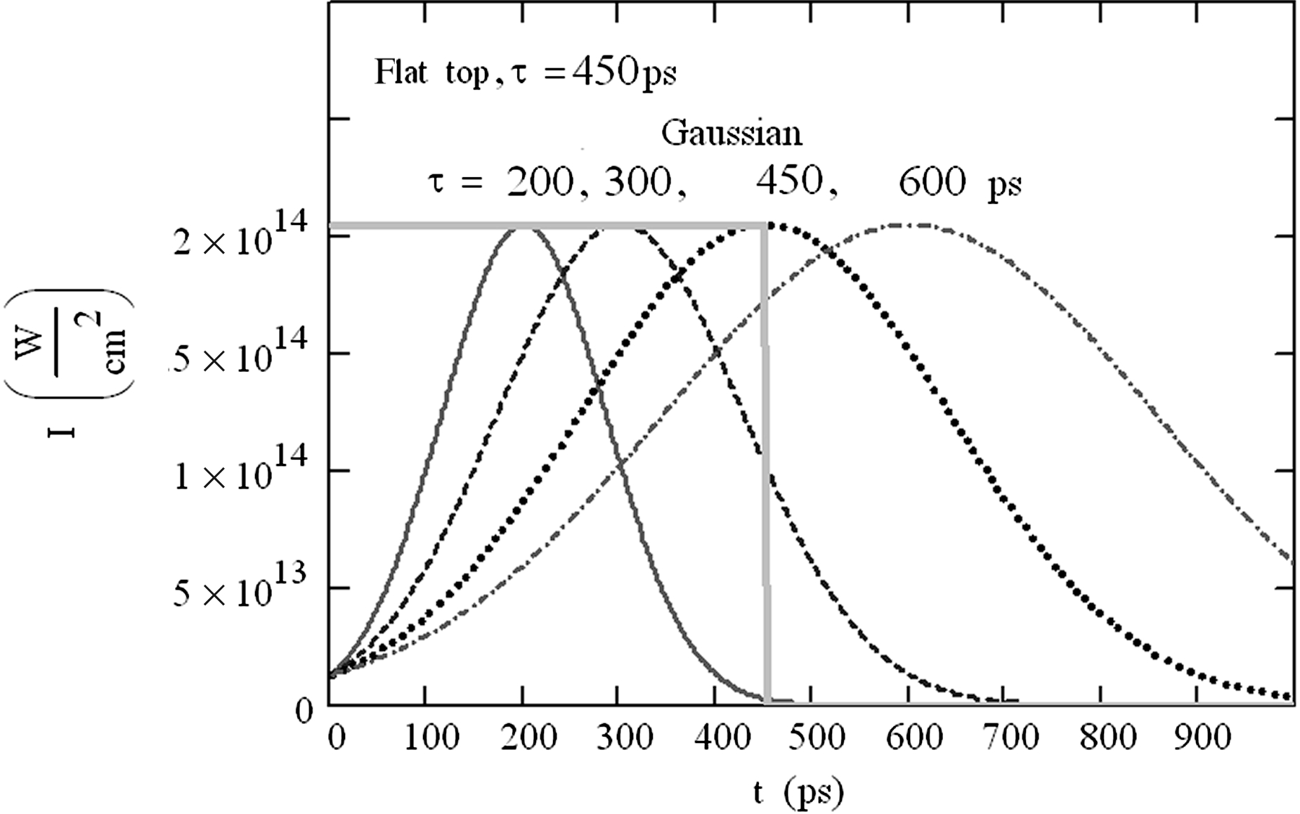
We have tested four Gaussian laser profiles with the same peak intensity ( ${I}_{\mathrm{max} } = 2. 05\times 1{0}^{14} ~\mathrm{W} / {\mathrm{cm} }^{2} $) and full width at half maximum (FWHM) durations $\tau = 200, 300, 450$, and 600 ps. Gaussian profiles were calculated by $I= {I}_{\mathrm{max} } \exp (- 2. 77\mathop{(\frac{t- \tau }{\tau } )}\nolimits ^{2} )$ (see Figure 3). So the initial intensity at zero time was 6.3% of the maximum. Also we used an ideal flat-top pulse of the same intensity and 450 ps duration for reference.
Figure 3. Laser pulse profiles used in the simulations.
3. Results and discussion
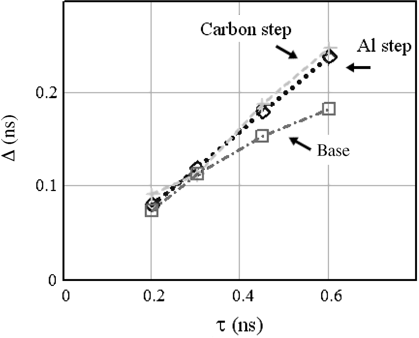
Figure 4 presents the dependence of the difference between shock arrivals for Gaussian pulses and the reference one (flat top) as a function of duration  $\tau $ for the three parts of the target.
Figure 4. The dependences of the difference between shock arrivals for Gaussian pulses and the reference one (flat top) from  $\tau $ for all three parts of the target: (i) base (Al: $8~\unicode[.5,0][STIXGeneral,Times]{x03BC} \mathrm{m} $); (ii) Al step (Al: $16. 5~\unicode[.5,0][STIXGeneral,Times]{x03BC} \mathrm{m} $); and (iii) carbon step (Al–C: $11. 5~\unicode[.5,0][STIXGeneral,Times]{x03BC} \mathrm{m} + 9. 5~\unicode[.5,0][STIXGeneral,Times]{x03BC} \mathrm{m} $) – ${ \mathrm{\Delta} }_{\mathrm{base} } , { \mathrm{\Delta} }_{\mathrm{Al} } $ and ${ \mathrm{\Delta} }_{\mathrm{C} } $, correspondingly. All dependences are very close to each other for $\tau \leqslant 300~\mathrm{ps} $.
If the rise-time of the Gaussian pulse is small ( $\tau \leqslant 300~\mathrm{ps} $ from Figure 4), the difference is the same for the base and both steps. This implies that the shock velocity calculations are not affected. Physically this means that for $\tau \leqslant 300~\mathrm{ps} $ the shock becomes stationary both in the base ( $8~\unicode[.5,0][STIXGeneral,Times]{x03BC} \mathrm{m} $ thick) and in the steps. In this case the effect of the Gaussian pulses is just to shift all breakout times by the same amount. We notice that these spatial profiles are not exactly the same (see Figure 5), but the same time differences for the shock breakouts are enough for a correct calculation of shock velocities.
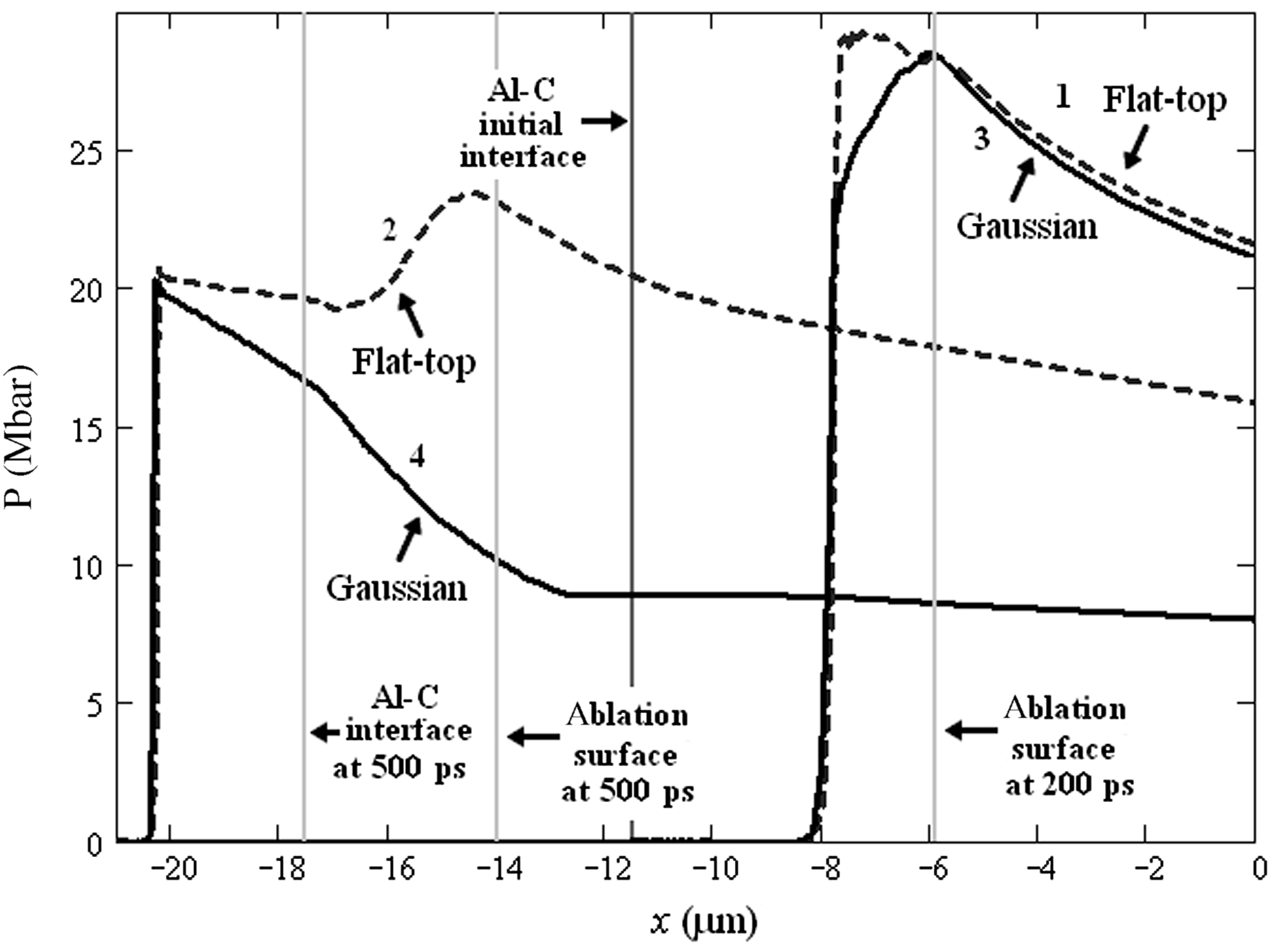
Figure 5. Comparison of spatial profiles for the shocks initiated by flat-top and Gaussian (FWHM duration 300 ps) pulses. Lines 1 and 2 (dashed) are shock profiles for a flat-top laser pulse at 200 and 500 ps (close to the shock breakout on the base and the carbon step). Lines 3 and 4 (solid) are shock profiles for a Gaussian laser pulse at 314 and 614 ps. We notice that both profiles have the same time shift  $ \mathrm{\Delta} = 114~\mathrm{ps} $. Despite the profile differences the fronts for both shocks are very close to each other. The laser strikes from the right. Zero on $x$ corresponds to the target front. The vertical line at $- 11. 5~\unicode[.5,0][STIXGeneral,Times]{x03BC} \mathrm{m} $ is the initial Al–C interface. Ablation surfaces and Al–C interfaces for flat-top profiles at 200 and 500 ps are indicated (for 200 ps, the Al–C interface is the initial one).
Simulations done for  $\tau \gt 300~\mathrm{ps} $ show that instead the shock has the time to become stationary in the steps (the difference is indeed the same for the two steps) but not for base. In this case the shock velocity cannot simply be calculated as $D= \text{thickness} / ({t}_{\mathrm{step} } - {t}_{\mathrm{base} } )$.
4. Conclusion
On the basis of hydro simulations, we can conclude that, with the considered laser intensity ( ${\approx }1{0}^{14} ~\mathrm{W} / {\mathrm{cm} }^{2} )$ and target design, it is necessary to have the duration of the Gaussian pulse not longer 300 ps. In the opposite case, the shock does not have the time to become stationary before the shock breaks out of the base. These results can be extrapolated to pulses with any shape by saying that the pulse rise-time should be less than 150 ps. Depending on target thickness, the pulse rise-time required will be different; however, the method described here is general.
Acknowledgements
The work was partially supported by ESF (SILMI, 3964), EU COST program, and RFBR (12-01-96500, 11-01-00707).

 Open access