


1. Introduction
The displacement of one fluid by another in porous media is one of the most common processes involving interfacial instabilities. It is generally accepted when the displacing fluid is more viscous that no interfacial instability occurs, while viscous fingering (VF) instability occurs in the reverse case. The latter case is hydrodynamically unfavourable, and the interface of the two fluids gives a finger-like pattern. This phenomenon is called Saffman–Taylor instability (Saffman & Taylor Reference Saffman and Taylor1958) or VF (Homsy Reference Homsy1987). The application of VF is widespread in several industrial and environmental processes such as chromatography (Mayfield et al. Reference Mayfield, Shalliker, Catchpoole, Sweeney, Wong and Guiochon2005), transport of digestive juices (Bhaskar et al. Reference Bhaskar, Grik, Turner, Bradley, Bansil, Stanley and LaMont1992), enhanced oil recovery (Lake et al. Reference Lake, Johns, Rossen and Pope2014),  $\mathrm {CO}_2$ sequestration (Orr & Taber Reference Orr and Taber1984) and frontal polymerization (Pojman et al. Reference Pojman, Gunn, Patterson, Owens and Simmons1998). Fluid–fluid miscibility plays an important role in VF dynamics, and the VF pattern can change appreciably based on the miscibility of the two fluids. Therefore, the subject is traditionally divided into immiscible and fully miscible VF. The mutual solubility is infinite in fully miscible systems, while it is zero in immiscible systems. Diffusion affects the VF dynamics in fully miscible systems. Thus, the fully miscible VF is characterized by the Péclet number $Pe$, defined as the ratio of convective transport rate and diffusive transport rate, $Pe = LV/D$, where $L$ is a characteristic length, $V$ is the flow velocity and $D$ is the diffusivity between the displacing and displaced fluids. On the other hand, interfacial tension affects the VF dynamics in immiscible systems. Thus, the immiscible VF is characterized by the capillary number $Ca$, defined as the ratio of viscous force and interfacial tension force, $Ca = \mu V / \gamma$, where ${\mu }$ is the viscosity of the more viscous fluid and ${\gamma }$ is the interfacial tension between the displacing and displaced fluids. In both types of VF, the dynamics is governed primarily by the viscosity contrast. The viscous fingers generally become thinner with increasing $Ca$ and $Pe$ (Chen Reference Chen1987; Nagatsu & Ueda Reference Nagatsu and Ueda2004; Pramanik & Mishra Reference Pramanik and Mishra2015a; Tsuzuki et al. Reference Tsuzuki, Ban, Fujimura and Nagatsu2019a,Reference Tsuzuki, Tanaka, Ban and Nagatsub). For the same viscosity contrast and flow rate, the fingers in immiscible systems are wider than those in miscible systems because the interfacial tension in immiscible systems can stabilize short-wavelength perturbations at the interface.
The interfacial tension between immiscible fluids is an equilibrium thermodynamic property resulting from the differences in intermolecular interactions between the two different types of molecules. In miscible systems, when the two non-premixed miscible fluids are brought in contact with each other, the initial concentration gradient between the two fluids immediately relaxes via diffusion, resulting in an equilibrated, uniform state. Therefore, in the case of two miscible fluids, there can be no interfacial tension at the interface of the fluids. However, in 1901, Korteweg proposed that a body force caused by a concentration (or density) gradient could act like an interfacial tension (Korteweg Reference Korteweg1901). On time scales shorter than that of interface relaxation, there does exist a capillary force at the interface because there are necessary differences in intermolecular interactions when the molecules are different. Such a capillary force is called Korteweg stress or effective interfacial tension (EIT) (Pojman et al. Reference Pojman, Whitmore, Liveri, Lombardo, Marszalek, Parker and Zoltowski2006; Zoltowski et al. Reference Zoltowski, Chekanov, Masere, Pojman and Volpert2007).
The effect of EIT on miscible VF dynamics has been numerically studied (Chen, Wang & Meiburg Reference Chen, Wang and Meiburg2001; Chen et al. Reference Chen, Huang, Gadelha and Miranda2008; Pramanik & Mishra Reference Pramanik and Mishra2013, Reference Pramanik and Mishra2014, Reference Pramanik and Mishra2015b; Swernath, Malengier & Pushpavanam Reference Swernath, Malengier and Pushpavanam2010). Chen et al. (Reference Chen, Huang, Gadelha and Miranda2008) showed that the miscible VF patterns in a radial geometry with EIT can be made to resemble the more familiar morphologies of their immiscible counterparts by increasing the value of a Korteweg stress parameter. Swernath et al. (Reference Swernath, Malengier and Pushpavanam2010) showed that Korteweg stress could stabilize miscible viscous fingers in a linear geometry and Pramanik & Mishra (Reference Pramanik and Mishra2013, Reference Pramanik and Mishra2014, Reference Pramanik and Mishra2015b) showed that Korteweg stress delays the onset of instability so that miscible viscous fingers are stabilized. In short, numerical studies have indicated that EIT can stabilize the Saffman–Taylor instability and that the fingers are wider due to the effect of EIT. Also, experimental studies of miscible VF with EIT have been reported. Truzzolillo et al. (Reference Truzzolillo, Mora, Dupas and Cipelletti2014) employed a method for estimating EIT from the patterns of miscible viscous fingers based on the assumption that EIT exists and showed that EIT is proportional to the square of volume fraction using a colloidal suspension and its own solvent (Truzzolillo et al. Reference Truzzolillo, Mora, Dupas and Cipelletti2014, Reference Truzzolillo, Mora, Dupas and Cipelletti2016; Truzzolillo & Cipelletti Reference Truzzolillo and Cipelletti2017).
In 2020, Suzuki et al. (Reference Suzuki, Quah, Ban, Mishra and Nagatsu2020) performed an experimental investigation of the effects of EIT on miscible VF by establishing two solution systems that have different EIT but the same viscosity contrast. They observed (i) that finger width with high EIT is larger than that with low EIT for the equivalent flow rate or  $Pe$ and (ii) that the finger width increases with the injection flow rate for low EIT. The reason for statement (ii) is explained by them as follows: the EIT value monotonically decreases with contact time of the two solutions and becomes nearly zero at the later stage. At the low flow rate, the EIT becomes very small or nearly zero when the VF pattern grows to a certain size because the contact time becomes long. At intermediate flow rates, the contact time is shorter until the VF pattern grows to a certain size, and the EIT maintains still a finite value even when the VF pattern grows to a certain size. Therefore, fingers are wider because of the EIT, which mimics an interfacial tension. At high flow rates, however, the finger width decreases with an increase in the flow rate (as in classical immiscible and miscible VF). This should be because the finger-thinning effect with an increase in the flow rate overcomes the finger-widening effect due to the interfacial tension.
It is well accepted that such finger widening with increasing flow rate is not observed in a classical immiscible or miscible system without EIT. Thus, such finger widening with increasing flow rate can be a peculiar characteristic of a miscible system with EIT. Therefore, it is important to theoretically analyse the influence of  $Pe$ (which corresponds to the injection flow rates in an experiment) on miscible viscous fingers with EIT. If such finger widening with increasing $Pe$ is theoretically reproduced, it is also important to clarify its origin. To this end, we numerically simulate the diffusion–convection equations coupled with Korteweg stress of miscible VF in porous media by varying $Pe$ and analyse the fingering patterns. We also discuss the one-dimensional EIT profile reconstructed by a one-dimensional diffusion–convection model for various $Pe$ to explain the effect of $Pe$ on miscible VF patterns with EIT.
This paper is organized as follows. The problem description and governing equations are given in § 2. The numerical results are described in §§ 3.1 and 3.2, and quantitative analysis and discussion are presented in § 3.3. Section 4 finally summarizes and concludes this study.
2. Problem description and governing equations
2.1. Physical problem
The system considered is a homogeneous porous medium or a Hele-Shaw cell with constant permeability  $k$, where an incompressible viscous fluid of viscosity $\mu _2$ ( $>\mu _1$) is placed initially (i.e. at time $t=0$) as shown in figure 1. The sample is displaced by another incompressible fluid of viscosity $\mu _1$ at a uniform velocity $U$ from the left domain. The two fluids are considered to be neutrally buoyant. The solvent concentration $c$, which drives viscosity $\mu (c)$ of the fluids, is assumed to be $c=0$ and $c=c_2$ in the displacing and displaced fluids, respectively. To take the EIT into consideration, it is assumed that the fluids diffuse at a slow rate so that the concentration gradient remains steep for a longer period in the thin mixing zone of the two fluids.

Figure 1. Sketch of a two-dimensional porous medium of length  $L_x$ and width $L_y$ with permeability $k$, where an incompressible fluid of viscosity $\mu _1$ displaces another of viscosity $\mu _2$ from left to right at a constant velocity $U$.
$U$.
2.2. Governing equations
The problem has been modelled by coupling the convection–diffusion equation for the solvent with the Darcy–Korteweg equation (Pramanik & Mishra Reference Pramanik and Mishra2013) for fluid flow velocity. Although the VF dynamics involving inertia effects by using Forchheimer's model (Joseph, Nield & Papanicolaou Reference Joseph, Nield and Papanicolaou1982) has recently been paid attention (Kim Reference Kim2022), we, here, investigate the effect of  $Pe$ on the VF dynamics by employing the Darcy–Korteweg equation, which has been used in several studies of VF with EIT. The model described by the Darcy–Korteweg equation can be governed by the following equations (Joseph & Renardy Reference Joseph and Renardy1992; Pramanik & Mishra Reference Pramanik and Mishra2013, Reference Pramanik and Mishra2014, Reference Pramanik and Mishra2015b; Swernath et al. Reference Swernath, Malengier and Pushpavanam2010):
 \begin{gather} \boldsymbol{\nabla}\boldsymbol{\cdot}\boldsymbol{u} = 0, \end{gather}
 \begin{gather} \boldsymbol{\nabla}[p+Q(c)] =-\frac{\mu}{k} \boldsymbol{u}+\boldsymbol{\nabla}\boldsymbol{\cdot}[\hat{\delta}(\boldsymbol{\nabla} c)(\boldsymbol{\nabla} c)], \end{gather}
 \begin{gather} \frac{\partial c}{\partial t} + \boldsymbol{u}\boldsymbol{\cdot}\boldsymbol{\nabla} c = D\nabla^2c, \end{gather}
 \begin{gather} \mu = \mu(c). \end{gather}
Equation (2.1) is the continuity equation or the mass conservation equation, which represents a solenoidal velocity field for incompressible fluids having velocity components  $\boldsymbol {u}=\boldsymbol {u}(u,v)$ along the $(x,y)$ directions. Equation (2.2) corresponds to the equation of motion or the momentum equation in the form of Darcy's law for the flow in porous media with a stress term, $\boldsymbol {\nabla }\boldsymbol {\cdot }[\hat {\delta }(\boldsymbol {\nabla } c)(\boldsymbol {\nabla } c)]$, for the EIT. Here $\hat {\delta }$ is called the Korteweg parameter. The transport of solvent is characterized by the convection–diffusion equation (2.3). It is noted that the pressure-like term $Q(c)$ due to Korteweg stress, appearing in the Darcy–Korteweg equation, can be defined as (Joseph & Renardy Reference Joseph and Renardy1992; Pramanik & Mishra Reference Pramanik and Mishra2013, Reference Pramanik and Mishra2014, Reference Pramanik and Mishra2015b; Swernath et al. Reference Swernath, Malengier and Pushpavanam2010)
 \begin{equation} Q(c) = \frac{\hat{\delta}}{3} \left[ \left( \frac{\partial c}{\partial x} \right)^2 + \left( \frac{\partial c}{\partial y} \right)^2 \right] - \frac{2\gamma}{3} \left( \frac{\partial^2c}{\partial x^2} + \frac{\partial^2c}{\partial y^2} \right), \end{equation}
where the parameter  $\gamma$ is a kind of gradient parameter (Swernath et al. Reference Swernath, Malengier and Pushpavanam2010). Both $\hat {\delta }$ and $\gamma$ depend on the compositions of the miscible mixture and need to be determined from experiments.
We used the moving frame method,  $x=x-Ut$ and $u=u-U\boldsymbol {e_x}$ (Tan & Homsy Reference Tan and Homsy1988). In order to obtain the non-dimensional form of the governing equations, we scale the flow velocity with $U$, time with $L_y/U$, viscosity with $\mu _1$, pressure with $\mu _1UL_y/k$ and concentration with $c_2$ following Pramanik & Mishra (Reference Pramanik and Mishra2015a). The non-dimensional governing equations are then obtained:
 \begin{equation} \boldsymbol{\nabla}\boldsymbol{\cdot}\boldsymbol{u} = 0, \end{equation}
 \begin{gather} \boldsymbol{\nabla} P =-\mu(c)(\boldsymbol{u}+\boldsymbol{i})+\boldsymbol{\nabla}\boldsymbol{\cdot}[\delta(\boldsymbol{\nabla} c)(\boldsymbol{\nabla} c)], \end{gather}
 \begin{gather} \frac{\partial c}{\partial t} + \boldsymbol{u}\boldsymbol{\cdot}\boldsymbol{\nabla} c = \frac{1}{Pe}\nabla^2c, \end{gather}
 \begin{gather} \mu(c) = e^{Rc}, \end{gather}
where  $R$ is the log-mobility ratio defined as $R=\ln (\mu _2/\mu _1)$, $\delta =\hat {\delta }kc_2^2/\mu _1UL_y^3$ is the non-dimensional Korteweg parameter, $\boldsymbol {i}$ representing the unit vector in the $x$ direction arises due to analysing in a moving reference frame and $Pe=UL_y/D$ is the Péclet number. Therefore, the term $\boldsymbol {\nabla }\boldsymbol {\cdot }[\delta (\boldsymbol {\nabla } c)(\boldsymbol {\nabla } c)]$ indicates the EIT. Taking the curl of the momentum equation and defining the stream function $\psi (x,y)$ as $u=\partial \psi /\partial y$ and $v=-\partial \psi /\partial x$ (Tan & Homsy Reference Tan and Homsy1988), we obtain
 \begin{gather}
\nabla^2\psi =-R\left(\frac{\partial\psi}{\partial
x}\frac{\partial c}{\partial x} +
\frac{\partial\psi}{\partial y}\frac{\partial c}{\partial
y} + \frac{\partial c}{\partial y} \right)\nonumber\\
- \frac{\delta}{\mu}\left[\frac{\partial c}{\partial
x}\left(\frac{\partial^3c}{\partial y\partial x^2} +
\frac{\partial^3c}{\partial y^3} \right) -\frac{\partial
c}{\partial y}\left(\frac{\partial^3c}{\partial x^3} +
\frac{\partial^3c}{\partial x \partial y^2} \right)
\right],
\end{gather}
\begin{gather}
\nabla^2\psi =-R\left(\frac{\partial\psi}{\partial
x}\frac{\partial c}{\partial x} +
\frac{\partial\psi}{\partial y}\frac{\partial c}{\partial
y} + \frac{\partial c}{\partial y} \right)\nonumber\\
- \frac{\delta}{\mu}\left[\frac{\partial c}{\partial
x}\left(\frac{\partial^3c}{\partial y\partial x^2} +
\frac{\partial^3c}{\partial y^3} \right) -\frac{\partial
c}{\partial y}\left(\frac{\partial^3c}{\partial x^3} +
\frac{\partial^3c}{\partial x \partial y^2} \right)
\right],
\end{gather} \begin{gather}
\frac{\partial c}{\partial t} +
\frac{\partial\psi}{\partial y}\frac{\partial c}{\partial
x} - \frac{\partial\psi}{\partial x}\frac{\partial
c}{\partial y} = \frac{1}{Pe}\nabla^2c.
\end{gather}
\begin{gather}
\frac{\partial c}{\partial t} +
\frac{\partial\psi}{\partial y}\frac{\partial c}{\partial
x} - \frac{\partial\psi}{\partial x}\frac{\partial
c}{\partial y} = \frac{1}{Pe}\nabla^2c.
\end{gather} We note that the stream function and vorticity formulation for both the present study and that of Seya et al. (Reference Seya, Suzuki, Nagatsu, Ban and Mishra2022) become the same although the physical basis for both works is different. The model systems are coupled partial differential equations in both the papers. Therefore, the species transport equation (3.2) in Seya et al. (Reference Seya, Suzuki, Nagatsu, Ban and Mishra2022) has the chemical potential function which shows the phase-separation effects. Whereas in the present paper, (2.11) contributes only to the effects of convection and diffusion of the species concentration. In both cases, there are additional stress terms which are due to the concentration gradient and chemical potential, for the present work (2.10) and for Seya et al. (Reference Seya, Suzuki, Nagatsu, Ban and Mishra2022) equation (3.1), respectively. The detailed derivations of such stream function–vorticity formulations are given in Appendices A and B. The dimensionless stream function–vorticity forms of (2.10) and (2.11) are numerically simulated using a pseudo-spectral method based on Fourier coefficients following Pramanik & Mishra (Reference Pramanik and Mishra2015a) and Tan & Homsy (Reference Tan and Homsy1988). Careful observation of the boundary conditions yields that the boundary conditions can be easily considered to be periodic without affecting the nature of the flow. Without loss of generality, the boundary conditions along the transverse boundaries can be considered periodic for computational purposes. However, in the longitudinal direction, the length of the computational domain is taken sufficiently large to take care of the periodic boundary conditions. Hence, the interfacial instability front is not affected by the boundary conditions. In the present study, we have employed the classical periodic boundary conditions, which have been used in many numerical studies on VF in rectilinear geometry, although it has been very recently reported that the transverse or lateral boundary conditions have an important role in VF dynamics (Kim & Pramanik Reference Kim and Pramanik2023). The computational domain is chosen to be  $[0,L_x/L_y]\times [0,1]$, where $L_x=8$ and $L_y=1$ with $1024\times 128$ spectra incorporated within a rectangular region. The time integration is performed by taking time stepping of $\Delta t=10^{-4}$. The convergence criteria are satisfied, similar to the results reported by Pramanik & Mishra (Reference Pramanik and Mishra2015a) with a different Fourier spectra size.
3. Results and discussion
3.1. Effect of EIT on the miscible VF dynamics
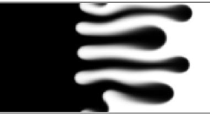
We firstly performed a numerical simulation of miscible VF to check the effect of EIT on the VF dynamics, the results of which are shown in figure 2. The parameter condition is  $R=0.75$ and $Pe=1000$. Comparing the case without EIT ( $\delta =0$), the fingers are wider as $|\delta |$ is larger. The onset time, when fingers appear or the interface becomes fluctuated, with EIT ( $\delta =-2\times 10^{-5}$) seems delayed compared with that without EIT. Also, finger length at a given time for $\delta =-2\times 10^{-5}$ seems shorter than that without EIT. Corresponding to such finger length, the mixing length $L$ has been studied (Tan & Homsy Reference Tan and Homsy1988). The length is defined here as the length of the transverse-averaged concentration field $\bar {c}(x,t)$ which lies in the range $0.01<\bar {c}(x,t)<0.99$. The quantitative data evaluated with the mixing length are shown in figure 3. The mixing length $L$ by diffusion grows proportional to $t^{1/2}$ until a finger appears. The $L$ value proportional to $t^1$ indicates finger appearance. Figure 3 quantitatively shows that the onset is delayed as $|\delta |$ is larger. The mixing length is shorter as $|\delta |$ is larger at a given time after the fingering formation. Therefore, the EIT has an influence on stabilizing VF dynamics at the same log-mobility ratio and the same $Pe$. These results are consistent with previous results reported by Swernath et al. (Reference Swernath, Malengier and Pushpavanam2010), Pramanik & Mishra (Reference Pramanik and Mishra2015b) and Chen et al. (Reference Chen, Huang, Gadelha and Miranda2008).

Figure 2. Time evolution of miscible VF dynamics (a) without EIT ( $\delta =0$) and with EIT ((b) $\delta =-10^{-6}$, (c) $\delta =-10^{-5}$, (d) $\delta =-2\times 10^{-5}$) for $R=0.75$ and $Pe=1000$. The greyscale shows the concentration of species.

Figure 3. Time evolution of mixing length for various  $\delta$ with $R=0.75$ and $Pe=1000$.
3.2. Effect of  $Pe$ on the miscible VF dynamics with/without EIT

We next performed a simulation to check the effect of  $Pe$ on the VF dynamics without/with EIT. The results without EIT shown in figure 4 illustrate that narrow and longer fingers appear as $Pe$ increases, the trend of which is the same as that of previously reported experimental and numerical results (Petitjeans et al. Reference Petitjeans, Chen, Meiburg and Maxworthy1999; Shukla & De Wit Reference Shukla and De Wit2020). The mixing length by diffusion at the early stage shown in figure 5 is smaller as $Pe$ increases because the concentration gradient is sharpened due to high $Pe$. At a later stage, the finger grows faster as $Pe$ increases after the onset time of the finger.

Figure 4. Time evolution of miscible VF dynamics without EIT ( $\delta =0$) for $R=1.25$, with (a) $Pe=500$,(b) $Pe=1000$, (c) $Pe=2500$ and (d) $Pe=3800$. The greyscale shows the concentration of species.

Figure 5. Time evolution of mixing length for various  $Pe$ with $\delta =0$ and $R=1.25$.
For the results with EIT ( $\delta =-2\times 10^{-5}$) shown in figure 6, the finger width shown at $t=26$ in figure 6(d) seems larger than that in figure 6(c). However, the quantitative data of mixing length shown in figure 7 represent a similar trend to the case without EIT in figure 5. In short, $L$ is smaller with $Pe$ at the early stage and $L$ grows faster with $Pe$ at a later stage. Compared with figure 5, figure 7 shows that the onset of the finger becomes later because of the EIT. We then directly measure the finger width to compare with the above experimental study. A detailed description is given in the next section.

Figure 6. Time evolution of miscible VF dynamics with EIT ( $\delta =-2\times 10^{-5}$) for $R=1.25$, with(a) $Pe=500$, (b) $Pe=1000$, (c) $Pe=2500$ and (d) $Pe=3800$. The greyscale shows the concentration of species.

Figure 7. Time evolution of mixing length for various  $Pe$ under conditions of $\delta =-2\times 10^{-5}$ and $R=1.25$.
3.3. Quantitative analysis of the finger width
We measured finger width density as quantitative data of the finger width to investigate the effect of  $Pe$ on the dynamics for various $R$ and $\delta$. The method is illustrated in figure 8. We first define the positive mixing length $L_+$, the length of a downstream finger propagating in the forward direction with respect to the initial interface (Manickam & Homsy Reference Manickam and Homsy1994). We then binarize the picture and calculate a finger width density $w_i$ at a position $x=i$ ( $0\le x\le L_+$) as
 \begin{equation} w_i = \frac{1}{j}\left(\frac{\varSigma w_j}{L_y} \right), \end{equation}
where  $w_j$ is a finger width coloured with black at $x=i$ (figure 8) and $j$ is the number of fingers. Then, we calculate an averaged finger width density for the fingering pattern over length $L$ (figure 8) using the following equation:
 \begin{equation} w = \frac{1}{L_+}\int^{L_+}_0 w_i \,{{\rm d}\kern0.7pt x}. \end{equation}
The measured results are shown in figure 9. For low EIT ( $\delta =-10^{-6}$) and without EIT, $w$ is monotonically decreasing against an increase in $Pe$ for any log-mobility ratios. For high-EIT cases ( $\delta =-10^{-5}$, $-2\times 10^{-5}$), however, the finger width decreases with $Pe$ for under $Pe=2000$ and increases as $Pe$ increases for over $Pe=2000$ for $R=0.75$ and 1.00. It is noted that the $w$ value does not increase against $Pe$ at $\delta =-10^{-5}$ for $R =1.25$. This is because the viscous term affects the VF dynamics more significantly compared with the effect of the EIT term at $R=1.25$ due to the large value of $R$. These results show that the finger widening on increasing the flow rate in the miscible system with EIT observed in the experiment (Suzuki et al. Reference Suzuki, Quah, Ban, Mishra and Nagatsu2020) can be numerically reproduced. Suzuki et al. (Reference Suzuki, Quah, Ban, Mishra and Nagatsu2020) explain such finger widening as being caused by the temporal effect of EIT, where the EIT value decreases with the contact time of the two fluids, as mentioned in the introductory section. However, we consider here that such finger widening is affected by the difference in EIT due to $Pe$, because EIT is proportional to the squared concentration gradient. Therefore, we examine the effect of $Pe$ on the concentration profile and the EIT term ( $\boldsymbol {\nabla }\boldsymbol {\cdot }[\delta (\boldsymbol {\nabla } c)(\boldsymbol {\nabla } c)]$) in the following discussion.

Figure 8. Sketch of the definition of finger width. (a) Definition of the positive mixing length and(b) description of finger width and coordinate.

Figure 9. Effect of  $Pe$ on finger width for (a) $R=0.75$, (b) $R=1.00$ and (c) $R=1.25$. Each colour represents a different EIT value. Each result is run three times and the error bar represents the standard deviation.
The concentration profile is calculated from the one-dimensional convection–diffusion equation (Shukla & De Wit Reference Shukla and De Wit2020):
 \begin{equation} \frac{\partial c}{\partial t} = \frac{1}{Pe}\frac{\partial^2c}{\partial x^2}. \end{equation}
As shown in figure 10(a), the concentration gradient at the interfacial front ( $x-x_0=0$) is steeper with $Pe$. Figure 10(b) shows the effect of $Pe$ on the EIT term with $R=1.00$ at $t=1$. As predicted, the EIT term is higher with $Pe$ because the concentration gradient is steeper with $Pe$. These results show that the finger widening with increasing $Pe$ in the present study is caused by an increase in the magnitude of EIT with increasing $Pe$. This is because $Pe$ induces a steeper concentration gradient, which induces higher EIT. We clarify here the relationship between this study and closely related studies (Pramanik & Mishra Reference Pramanik and Mishra2015a,Reference Pramanik and Mishrab). Pramanik & Mishra (Reference Pramanik and Mishra2015b) have investigated VF with EIT at fixed $Pe$ and have shown the miscible VF with EIT is determined to be stable only in terms of onset and moving speed without any discussion about the effects of $Pe$. The present study completely follows the mathematical model and the boundary condition of Pramanik & Mishra (Reference Pramanik and Mishra2015a). Pramanik & Mishra (Reference Pramanik and Mishra2015a) have conducted a linear stability analysis of miscible VF with EIT. However, they have studied neither nonlinear dynamics of VF with EIT nor the relation between finger width in the nonlinear regime and $Pe$. The present study is the first study which numerically investigates the effects of $Pe$ on nonlinear VF with EIT. And the present study numerically demonstrates, for the first time, finger widening against increasing $Pe$ in VF with EIT, which has not been seen either in immiscible VF or in miscible VF without EIT.

Figure 10. (a) Concentration profile for various  $Pe$ at $t =1$ and (b) the value of EIT term $\boldsymbol {\nabla }\boldsymbol {\cdot }[\delta (\boldsymbol {\nabla } c)(\boldsymbol {\nabla } c)]$ with $\delta =-2\times 10^{-5}$ calculated based on (a).
Finally, we estimate EIT values to determine whether our setting parameters are feasible in experiments. The term  $\hat {\delta }\boldsymbol {\cdot }(\Delta c)^2/\delta _{interface}$ represents ‘EIT value $({\rm N}\,{\rm m}^{-1})$’ (Truzzolillo et al. Reference Truzzolillo, Mora, Dupas and Cipelletti2014). We thus calculate $\hat {\delta }\boldsymbol {\cdot }(\Delta c)^2/\delta _{interface}$ with the relation $\delta =\hat {\delta }kc_2^2/\mu _1UL_y^3$, $Pe=UL_y/D$ and $k=b^2/12$ with $\delta _{interface}=100\,\mathrm {\mu }{\rm m}$ (Zoltowski et al. Reference Zoltowski, Chekanov, Masere, Pojman and Volpert2007), $c_2=1, \Delta c=1, L_y=50\times 10^{-3}\,{\rm m}, D=1.6\times 10^{-10}\,{\rm m}^2\,{\rm s}^{-1}$ (Petitjeans & Maxworthy Reference Petitjeans and Maxworthy1996), $\mu _1=0.001\,{\rm Pa}\,{\rm s}$ and $b=0.5\times 10^{-3}\,{\rm m}$, where $b$ is the gap between Hele-Shaw cells and $\delta _{interface}$ is the interface width between the two solutions:
 \begin{equation} \hat{\delta}\boldsymbol{\cdot}\frac{(\Delta c)^2}{\delta_{interface}} = \frac{\delta\mu_1 (Pe\boldsymbol{\cdot} D)L_y^2}{(b^2/12)c_2^2}\boldsymbol{\cdot} \frac{(\Delta c)^2}{\delta_{interface}}=1.92\times10^{{-}4}\boldsymbol{\cdot}|\delta|\boldsymbol{\cdot} Pe. \end{equation}
Based on this expression, the EIT value is  $7.30\times 10^{-3}\,{\rm mN}\,{\rm m}^{-1}$ with, for example, $Pe=3800$ and $|\delta |=10^{-5}$. Therefore, the set values of $\delta$ here should be ‘very low’ interfacial tensions in experiments (Bamberger et al. Reference Bamberger, Seaman, Sharp and Brooks1984; Liu, Lipowsky & Dimova Reference Liu, Lipowsky and Dimova2012; Carbonaro, Cipelletti & Truzzolillo Reference Carbonaro, Cipelletti and Truzzolillo2020).
4. Conclusions
In conclusion, we investigate the effect of  $Pe$ on miscible VF with/without EIT using a numerical simulation. The increase in the finger width with increasing $Pe$ is observed with EIT. The results confirm the recent experimental finding that a finger widens on increasing the flow rate in the miscible VF with EIT (Suzuki et al. Reference Suzuki, Quah, Ban, Mishra and Nagatsu2020). In this study, we also analysed the one-dimensional underlying concentration profile and EIT profile by using the one-dimensional diffusion–convection model because EIT is proportional to the squared concentration gradient. We then obtained that the concentration gradient is steeper with an increase in $Pe$, resulting in a larger EIT with $Pe$. Based on the one-dimensional analysis, the finger widening with increasing $Pe$ obtained by the numerical simulation can be caused by an increase in the concentration gradient, resulting in an increase in EIT with $Pe$.
$Pe$.
The present study theoretically verifies that finger widening with increasing flow rate occurs only in the miscible system with EIT to the extent of our targeting EIT values, also clarifying its origin. These findings will trigger further experimental, numerical and theoretical studies of the manifested influence of EIT on miscible VF because the finger width is affected by EIT and  $Pe$. In addition, our study will provide a theoretical framework to control miscible VF in many geophysical processes such as $\mathrm {CO}_2$ sequestration (Orr & Taber Reference Orr and Taber1984) and miscible flooding in enhanced oil recovery (Lake et al. Reference Lake, Johns, Rossen and Pope2014).
Acknowledgements
The authors thank Dr T. Ban, Osaka University for fruitful discussions. M.M. gratefully acknowledges the JSPS Invitation Fellowships for Research in Japan (no. L19548).
Funding
This work was supported by JSPS KAKENHI grant nos. 22K03900 and 22K20402 and by JST Presto grant no. JPMJPR22O5.
Declaration of interests
The authors report no conflict of interest.
Appendix A. Derivation of stream function and vorticity formulation in the present study
Equations (2.6) and (2.7) can be expressed in component-wise manner as
 \begin{gather} \frac{\partial u}{\partial x} + \frac{\partial v}{\partial y} = 0, \end{gather}
 \begin{gather} \frac{\partial p}{\partial x} =-\mu(c) (u + 1) + \frac{\partial}{\partial x}\left[\delta \left(\frac{\partial c}{\partial x} + \frac{\partial c}{\partial y} \right)\left(\frac{\partial c}{\partial x} + \frac{\partial c}{\partial y} \right) \right], \end{gather}
 \begin{gather} \frac{\partial p}{\partial y} =-\mu (c) v + \frac{\partial}{\partial y}\left[\delta \left(\frac{\partial c}{\partial x} + \frac{\partial c}{\partial y} \right)\left(\frac{\partial c}{\partial x} + \frac{\partial c}{\partial y} \right) \right]. \end{gather}
 Eliminating the pressure term from the above (A2) and (A3) by cross-differentiation with respect to  $y$ and $x$, respectively, and subtracting (A3) from (A2), we get
 \begin{align} &\mu(c) \left(
-\frac{\partial v}{\partial x} + \frac{\partial u}{\partial
y} \right) -v\frac{\partial\mu(c)}{\partial x} +
(u+1)\frac{\partial\mu}{\partial y} \nonumber\\ &\quad+
\delta \left[ \frac{\partial c}{\partial x} \left(
\frac{\partial^3c}{\partial x^2 \partial y} +
\frac{\partial^3c}{\partial y^3} \right) - \frac{\partial
c}{\partial y} \left( \frac{\partial^3c}{\partial x^3} +
\frac{\partial^3c}{\partial x \partial y^2} \right)
\right]=0.
\end{align}
\begin{align} &\mu(c) \left(
-\frac{\partial v}{\partial x} + \frac{\partial u}{\partial
y} \right) -v\frac{\partial\mu(c)}{\partial x} +
(u+1)\frac{\partial\mu}{\partial y} \nonumber\\ &\quad+
\delta \left[ \frac{\partial c}{\partial x} \left(
\frac{\partial^3c}{\partial x^2 \partial y} +
\frac{\partial^3c}{\partial y^3} \right) - \frac{\partial
c}{\partial y} \left( \frac{\partial^3c}{\partial x^3} +
\frac{\partial^3c}{\partial x \partial y^2} \right)
\right]=0.
\end{align} Introducing the vorticity ( $\bar {\omega } = \boldsymbol {\nabla } \times \boldsymbol{u}$), for two-dimensional flow in the $x$–
$x$– $y$ plane, it is reduced to $\omega _z = \omega ={\partial v}/{\partial x} - {\partial u}/{\partial y}$. Further, using the vorticity, the above equation (A4) can be written as
 \begin{align} &{-}{\mu} (c) \omega -v\frac{\partial\mu(c)}{\partial x} + (u+1)\frac{\partial\mu(c)}{\partial y} \nonumber\\ &\quad +\delta \left[ \frac{\partial c}{\partial x} \left( \frac{\partial^3c}{\partial x^2 \partial y} + \frac{\partial^3c}{\partial y^3} \right) - \frac{\partial c}{\partial y} \left( \frac{\partial^3c}{\partial x^3} + \frac{\partial^3c}{\partial x \partial y^2} \right) \right]=0. \end{align}
From the viscosity–concentration relation (2.9), we can write
 $$\begin{gather} \frac{\partial\mu(c)}{\partial x} = \frac{\partial\mu(c)}{\partial c}\frac{\partial c}{\partial x} = R\mu(c) \frac{\partial c}{\partial x}, \end{gather}$$
 $$\begin{gather}\frac{\partial\mu(c)}{\partial y} = \frac{\partial\mu(c)}{\partial c}\frac{\partial c}{\partial y} = R\mu(c) \frac{\partial c}{\partial y}. \end{gather}$$
 Introducing the stream function  $\psi$ as ( $u = {\partial \psi }/{\partial y}$ and $v = -({\partial \psi }/{\partial x})$), satisfying (A1), we have $\nabla ^2\psi = -\omega$. Using (A6), (A7) and the above stream function–vorticity relation, equation (A5) becomes
 \begin{align} \nabla^2\psi &=-R \left( \frac{\partial \psi}{\partial x}\frac{\partial c}{\partial x} + \frac{\partial\psi}{\partial y} +\frac{\partial c}{\partial y} \right) \nonumber\\ &\quad- \frac{\delta}{\mu(c)} \left[ \frac{\partial c}{\partial x} \left( \frac{\partial^3c}{\partial x^2 \partial y} + \frac{\partial^3c}{\partial y^3} \right) - \frac{\partial c}{\partial y} \left( \frac{\partial^3c}{\partial x^3} + \frac{\partial^3c}{\partial x \partial y^2} \right) \right]. \end{align}
Appendix B. Derivation of stream function and vorticity formulation in the study reported by Seya et al. (2022)
The non-dimensional equations (2.8)–(2.12) of Seya et al. (Reference Seya, Suzuki, Nagatsu, Ban and Mishra2022), in the moving frame and component-wise, can be read as
 $$\begin{gather} \frac{\partial u}{\partial x} + \frac{\partial v}{\partial y} = 0, \end{gather}$$
 $$\begin{gather}\frac{\partial p}{ \partial x} =-\eta(c)(u + 1) + \delta\mu(c,p)\frac{\partial c}{\partial x}, \end{gather}$$
 $$\begin{gather}\frac{\partial p}{\partial y} =-\eta(c) v + \delta\mu(c,p)\frac{\partial c}{\partial y}, \end{gather}$$
 $$\begin{gather}\frac{\partial c}{\partial t} + \boldsymbol{u}\boldsymbol{\cdot}\boldsymbol{\nabla} c = \frac{1}{Pe}\nabla^2 \mu(c,p), \end{gather}$$
 $$\begin{gather}\mu(c,p) =-\alpha_1 \left( \frac{\partial^2 c}{\partial x^2} + \frac{\partial^2 c}{\partial x^2} \right) - \alpha_2 (c-p) + \alpha_3 (c-p)^3, \end{gather}$$
 $$\begin{gather}\eta(c) = e^{Rc}. \end{gather}$$
 Eliminating the pressure term from the above equations (B2) and (B3) by cross-differentiation with respect to  $y$ and $x$, respectively, and subtracting (B3) from (B2), we get
 \begin{align} \eta(c)\left(-\frac{\partial v}{\partial x} +\frac{\partial u}{\partial y} \right)-v\frac{\partial\eta(c)}{\partial x}+ (u+1)\frac{\partial \eta(c)}{\partial y}+ \delta\frac{\partial\mu(c,p)}{\partial x}\frac{\partial c}{\partial y}- \delta\frac{\partial\mu(c,p)}{\partial y}\frac{\partial c}{\partial x}=0. \end{align}
 Similar to the explanation in Appendix A, using the vorticity for two-dimensional flow in the  $x$–
$x$– $y$ plane, $\omega _z = \omega ={\partial v}/{\partial x} - {\partial u}/{\partial y}$, in the above equation (B7), we get
 \begin{equation} {-}{\eta(c)}\omega-v\frac{\partial\eta(c)}{\partial x}+ (u+1)\frac{\partial \eta(c)}{\partial y}+ \delta\frac{\partial\mu(c,p)}{\partial x}\frac{\partial c}{\partial y}- \delta\frac{\partial\mu(c,p)}{\partial y}\frac{\partial c}{\partial x}=0. \end{equation}
 With the definition of the viscosity ( $\eta (c)=e^{Rc}$), we can write
 $$\begin{gather} \frac{\partial\eta(c)}{\partial x} = \frac{\partial\eta(c)}{\partial c}\frac{\partial c}{\partial x} = R\eta(c) \frac{\partial c}{\partial x}, \end{gather}$$
 $$\begin{gather}\frac{\partial\eta(c)}{\partial y} = \frac{\partial\eta(c)}{\partial c}\frac{\partial c}{\partial y} = R\eta(c) \frac{\partial c}{\partial y}. \end{gather}$$
Hence, using relations (B9) and (B10), after simplifying, (B8) can be written as
 \begin{equation} \omega = R\left({-}v\frac{\partial c}{\partial x}+ u\frac{\partial c}{\partial y} + \frac{\partial c}{\partial y}\right)+ \frac{\delta}{\eta(c)}\left(\frac{\partial\mu(c,p)}{\partial x}\frac{\partial c}{\partial y}- \frac{\partial\mu(c,p)}{\partial y}\frac{\partial c}{\partial x}\right). \end{equation}
 Using the stream function  $\psi$ as ( $u = {\partial \psi }/{\partial y}$ and $v = -({\partial \psi }/{\partial x})$), we write the above equation as
 \begin{equation} \omega = R\left(\frac{\partial\psi}{\partial x}\frac{\partial c}{\partial x}+ \frac{\partial\psi}{\partial y}\frac{\partial c}{\partial y} + \frac{\partial c}{\partial y}\right)+ \frac{\delta}{\eta(c)}\left(\frac{\partial\mu(c,p)}{\partial x}\frac{\partial c}{\partial y}- \frac{\partial\mu(c,p)}{\partial y}\frac{\partial c}{\partial x}\right). \end{equation}
Further, we simplify the second term on the right-hand side of the above equation (B12) as per the following:
 \begin{align} \frac{\partial\mu(c,p)}{\partial x} &= \frac{\partial}{\partial x}\left\{ -\alpha_1 \left(\frac{\partial^2 c}{\partial x^2} + \frac{\partial^2 c}{\partial y^2} \right) - \alpha_2 (c-p) + \alpha_3 (c-p)^3 \right\}\nonumber\\ &=-\alpha_1 \frac{\partial}{\partial x}\left( \frac{\partial^2 c}{\partial x^2} + \frac{\partial^2 c}{\partial y^2} \right) - \alpha_2 \frac{\partial c}{\partial x} + \alpha_3 \frac{\partial (c-p)^3}{\partial x}, \end{align}
 \begin{align} \frac{\partial\mu(c,p)}{\partial x}\frac{\partial c}{\partial y} &= \left\{-\alpha_1 \frac{\partial}{\partial x}\left( \frac{\partial^2 c}{\partial x^2} + \frac{\partial^2 c}{\partial y^2} \right) - \alpha_2 \frac{\partial c}{\partial x} + \alpha_3 \frac{\partial (c-p)^3}{\partial x} \right\} \frac{\partial c}{\partial y} \nonumber\\ &=-\alpha_1 \left( \frac{\partial^3 c}{\partial x^3} + \frac{\partial^3 c}{\partial x \partial y^2} \right) \frac{\partial c}{\partial y} - \alpha_2 \frac{\partial c}{\partial x}\frac{\partial c}{\partial y} + \alpha_3 \frac{\partial (c-p)^3}{\partial x}\frac{\partial c}{\partial y} \nonumber\\ &=-\alpha_1 \left( \frac{\partial^3 c}{\partial x^3} + \frac{\partial^3 c}{\partial x \partial y^2} \right) \frac{\partial c}{\partial y} - \alpha_2 \frac{\partial c}{\partial x}\frac{\partial c}{\partial y} + \alpha_3 \frac{\partial (c-p)^3}{\partial c}\frac{\partial c}{\partial x}\frac{\partial c}{\partial y}, \end{align}
 \begin{align} \frac{\partial\mu(c,p)}{\partial y} &= \frac{\partial}{\partial y}\left\{ -\alpha_1 \left(\frac{\partial^2 c}{\partial x^2} + \frac{\partial^2 c}{\partial y^2} \right) - \alpha_2 (c-p) + \alpha_3 (c-p)^3 \right\} \nonumber\\ &=-\alpha_1 \frac{\partial}{\partial y}\left(\frac{\partial^2 c}{\partial x^2} + \frac{\partial^2 c}{\partial y^2} \right) - \alpha_2 \frac{\partial c}{\partial y} + \alpha_3 \frac{\partial (c-p)^3}{\partial y} \end{align}
and
 \begin{align} \frac{\partial\mu(c,p)}{\partial y}\frac{\partial c}{\partial x} &= \left\{-\alpha_1 \frac{\partial}{\partial y}\left( \frac{\partial^2 c}{\partial x^2} + \frac{\partial^2 c}{\partial y^2} \right) - \alpha_2 \frac{\partial c}{\partial y} + \alpha_3 \frac{\partial (c-p)^3}{\partial y} \right\} \frac{\partial c}{\partial x} \nonumber\\ &=-\alpha_1 \left( \frac{\partial^3 c}{\partial x^2 \partial y} + \frac{\partial^3 c}{\partial y^3} \right) \frac{\partial c}{\partial x} - \alpha_2 \frac{\partial c}{\partial x}\frac{\partial c}{\partial y} + \alpha_3 \frac{\partial (c-p)^3}{\partial y}\frac{\partial c}{\partial x} \nonumber\\ &=-\alpha_1 \left( \frac{\partial^3 c}{\partial x^2 \partial y} + \frac{\partial^3 c}{\partial y^3} \right) \frac{\partial c}{\partial x} - \alpha_2 \frac{\partial c}{\partial x}\frac{\partial c}{\partial y} + \alpha_3 \frac{\partial (c-p)^3}{\partial c}\frac{\partial c}{\partial x}\frac{\partial c}{\partial y}. \end{align}
Using (B14) and (B16), (B12) can be expressed as
 \begin{align} \omega = R \left( \frac{\partial \psi}{\partial x}\frac{\partial c}{\partial x} + \frac{\partial\psi}{\partial y} +\frac{\partial c}{\partial y} \right) + \frac{\delta\alpha_1}{\eta(c)} \left[ \frac{\partial c}{\partial x} \left( \frac{\partial^3c}{\partial x^2 \partial y} + \frac{\partial^3c}{\partial y^3} \right) - \frac{\partial c}{\partial y} \left( \frac{\partial^3c}{\partial x^3} + \frac{\partial^3c}{\partial x \partial y^2} \right) \right]. \end{align}
Thus, we get
 \begin{align} \nabla^2\psi &=-R \left( \frac{\partial \psi}{\partial x}\frac{\partial c}{\partial x} + \frac{\partial\psi}{\partial y} +\frac{\partial c}{\partial y} \right) \nonumber\\ &\quad - \frac{\delta\alpha_1}{\eta(c)} \left[ \frac{\partial c}{\partial x} \left( \frac{\partial^3c}{\partial x^2 \partial y} + \frac{\partial^3c}{\partial y^3} \right) - \frac{\partial c}{\partial y} \left( \frac{\partial^3c}{\partial x^3} + \frac{\partial^3c}{\partial x \partial y^2} \right) \right], \end{align}
because of  $\nabla ^2\psi = -\omega$. The above equation is the stream function–vorticity equation (3.1) of Seya et al. (Reference Seya, Suzuki, Nagatsu, Ban and Mishra2022).


 Open access