


1. Introduction
The general equation of motion for fluid flow is the Navier–Stokes equation, with or without a force field term. If included, the force density term  $\boldsymbol f$ is often assumed to be conservative by which its impact is included in the pressure term (Batchelor Reference Batchelor1970). This approach is used in most aerodynamic analyses, where the flow is solved using the equation of motion without the force field term. When the flow is solved, the pressure is known, so the load on the body follows by integration of the pressure over the surface of the body. In other words, the load is the output. An alternative approach is proposed by Prandtl (Reference Prandtl1918), in which the force field term is maintained, representing the action of lifting bodies, without the need to define it as conservative. The force field acts on the surface of the lifting body, modelled as a vortex sheet. The force field is considered as an externally defined force field, and is input in the analyses: the force field determines the flow. In the remainder of the paper this method is named the force field method. Both approaches are consistent as shown by Prandtl (Reference Prandtl1918). The first approach is at the basis of most analytical and numerical analyses, and made great achievements possible, as described by Wu, Ma & Zhou (Reference Wu, Ma and Zhou2005, § 11.1.2) having the title ‘The Legacy of Pioneering Aerodynamicists’. The force field method has been detailed by von Kármán & Burgers (Reference von Kármán and Burgers1935), proposing an implementation scheme for calculations. Pioneers in rotor analyses like Froude (Reference Froude1889), Betz (Reference Betz1920) and Joukowsky (Reference Joukowsky1920), already used prescribed force fields in the development of the actuator disc theory, based on momentum and energy conservation laws. von Kármán & Burgers (Reference von Kármán and Burgers1935) used an intermittently operating disc force field to analyse the generation of vortex rings. Taylor (Reference Taylor1953) used the impulse imparted to the flow by a moving but suddenly dissolving disc to derive vortex ring parameters. Still the force field method did not become a favourite method until the interest in modern wind energy triggered new research and analysis of rotors. Madsen et al. (Reference Madsen, Larsen, Paulsen and Vita2013) used the implementation of von Kármán & Burgers (Reference von Kármán and Burgers1935) for actuator cylinder analyses, but the force field method has become most powerful in the analyses of the wake behind a wind turbine rotor. The rotor blades are replaced by a distribution of forces acting at a line representing the blade. The reason to do so is that this actuator line method allows a fast computation of the wake when details of the wake flow are more important than details of the blade flow. The disadvantage of this approach is that the force field needs to be known in advance of the analysis, which is not always the case. The first publication on this method is Sørensen & Shen (Reference Sørensen and Shen2002), whereas Asmuth, Olivares-Espinosa & Ivanell (Reference Asmuth, Olivares-Espinosa and Ivanell2020) present a recent paper with an extensive bibliography. A first application in helicopter rotor analysis is found in Merabet & Laurendeau (Reference Merabet and Laurendeau2021). The state of the art in actuator disc theory, using forces as input, is published by van Kuik (Reference van Kuik2018).
Despite the renewed interest in using force fields as source terms, there is little research on the question of whether a lifting body force field is conservative or non-conservative. The review paper on aerodynamic forces by Wu, Liu & Liu (Reference Wu, Liu and Liu2018) does not discuss this subject, and books on vorticity dynamics (Saffman Reference Saffman1992; Wu et al. Reference Wu, Ma and Zhou2005; Wu, Ma & Zhou Reference Wu, Ma and Zhou2015) treat it incidentally. Saffman (Reference Saffman1992) limits the force field generally to conservative fields, although on p. 53 he states that a non-conservative force field is required to generate instantaneously a motion from rest. Wu et al. (Reference Wu, Ma and Zhou2005, p. 132) accept as non-conservative force field the Coriolis force in a rotating frame of reference and the Lorentz force in magneto-hydrodynamics, and emphasise the role of ‘non-conservative body forces in affecting the flow development through its interaction with the vorticity field’. Wu et al. (Reference Wu, Ma and Zhou2015, p. 119) mention the Coriolis force as a non-conservative force.
Although the force field method is not often used, its original publication (Prandtl Reference Prandtl1918) is famous for the derivation of the Kutta–Joukowsky load, considered by Wu et al. (Reference Wu, Liu and Liu2018) as ‘the best of all kind of derivations’. The present paper brings this method back to the fore: the body is replaced by a flow contour within which the fluid is at rest relative to the contour of the domain. The contour has become a load carrying vortex sheet, with the load being the pressure jump across the sheet. This load is used as a force field source term in the Euler equation of motion.
The classification of body force fields as conservative or non-conservative is the new element in the analysis, leading to new interpretations of the relations between forces and work, forces and vorticity, and the relation between bound and trailing vorticity of a wing. The first objective is to show which force field generates vorticity in ideal flows and converts mechanical energy. The second objective is to show that the force field method reproduces the well-known relations between bound vorticity and (the absence of) trailing vorticity of an aerofoil and similarly between bound and trailing vorticity of a wing.
The paper is structured as follows.
(i) § 2 presents the force field approach of Prandtl, but with the body force fields allowed to be conservative or non-conservative, leading to a conservative or non-conservative interpretation of the Euler equation.
(ii) § 3 analyses how the generation or conservation of vorticity and the conversion or conservation of energy are linked to these non-conservative or conservative force fields.
(iii) In § 4 the distinction is made which lifting body force field distribution is conservative or non-conservative.
(iv) § 5 gives the derivation of the Kutta–Joukowsky load as part of the analysis how bound and trailing vorticity are connected, expressed in force field properties.
(v) § 6 analyses the relation between conservative forces, potential and potential energy, and similarly between non-conservative forces and the theorems of Helmholtz.
(vi) Finally § 7 presents the conclusions.
2. The Euler equation including the body force field
2.1. Prandtl's method
The derivation in this subsection is based on Prandtl (Reference Prandtl1918). The analysis is restricted to inviscid, incompressible flow, with ’inviscid’ understood as ’effectively inviscid’ (Batchelor Reference Batchelor1970, chapter 7). The equation of motion for such an ideal flow is the Navier–Stokes equation for vanishing viscosity, resulting in the Euler equation (Prandtl Reference Prandtl1918, eq. 2)
 \begin{equation} \rho\frac{{\rm D} \boldsymbol{v}}{{\rm D} t}={-}\boldsymbol{\nabla}p+\boldsymbol{f}, \end{equation}
in which  $\rho$ is the mass density, $\boldsymbol v$ the velocity vector, $p$ the pressure and $\boldsymbol f$ the force density which is invariant in time. Furthermore, the continuity equation holds,
 \begin{equation} \boldsymbol{\nabla}\boldsymbol{\cdot} \boldsymbol{v}=0. \end{equation}
 An alternative version of (2.1) is derived with  ${{\rm D} \boldsymbol {v}}/{{\rm D} t}={\partial \boldsymbol {v}}/{\partial t}+( \boldsymbol {v}\boldsymbol {\cdot } \boldsymbol {\nabla }) \boldsymbol {v}$ and the vector identity $( \boldsymbol {v}\boldsymbol {\cdot }\boldsymbol {\nabla }) \boldsymbol {v}=\frac {1}{2}\nabla ( \boldsymbol {v}\boldsymbol {\cdot } \boldsymbol {v})-\boldsymbol {v} \boldsymbol{\times} \boldsymbol {\omega }$, where $\boldsymbol {\omega } =\boldsymbol {\nabla } \boldsymbol{\times} \boldsymbol {v}$ is the vorticity,
 \begin{equation} \boldsymbol{\nabla} H=\boldsymbol{f}-\rho\frac{\partial\boldsymbol{v}}{\partial t}+\rho\boldsymbol{v} \boldsymbol{\times} \boldsymbol{\omega}, \end{equation}
with  $H$ being the steady Bernoulli parameter $p+\frac {1}{2}\rho \boldsymbol {v}\boldsymbol {\cdot } \boldsymbol {v}$, expressing the energy in the flow.
When  $\boldsymbol f$ is a normal force field distributed on a thin surface having thickness $\epsilon$ and behaves as a Dirac delta function, integration across the thickness $\epsilon$ and taking the limit of $\epsilon \rightarrow 0$ turn it into a normal surface load $F$ with the unit of pressure
 \begin{equation} \boldsymbol F=\lim_{\epsilon \rightarrow 0}\int_{\epsilon} \boldsymbol f \,{\rm d}n, \end{equation}
with  $n$ being normal to the surface. This procedure is equivalent to defining the lifting surface as a vortex sheet $\boldsymbol \gamma$ being the result of distribution of vorticity $\boldsymbol \omega$ on a layer with thickness $\epsilon$ in the limit of vanishing $\epsilon$,
 \begin{equation} \boldsymbol \gamma=\lim_{\epsilon \rightarrow 0}\int_{\epsilon} \boldsymbol \omega\,{\rm d}n. \end{equation}
An example of a distribution of  $\boldsymbol F$ is shown in figure 1, being the pressure distribution on an aerofoil. In the force field method the load distribution $\boldsymbol F$ is prescribed at the position of the aerofoil contour, without the aerofoil being present as a body. Further limit transitions are possible: if the height of the contour goes to zero, the contour becomes an infinitely thin surface, equivalent to a vortex sheet. Moreover, when the chord shrinks to zero, the contour becomes a load carrying point, equivalent to a discrete vortex.

Figure 1. The normal force field  $\boldsymbol F$ representing the pressure distribution at the surface of an aerofoil.
2.2. Conservative and non-conservative forces
Using Helmholtz's decomposition,  $\boldsymbol {f}$ can be distinguished in conservative and non-conservative force fields: $\boldsymbol {f}=\boldsymbol {f}_{cons}+\boldsymbol {f}_{non\text {-}cons}$, defined by the properties,
 \begin{equation} \left. \begin{array}{l} \boldsymbol{\nabla} \boldsymbol{\times} \boldsymbol{f}_{non\text{-}cons}\neq0 ,\\ \boldsymbol f _{cons}={-}\boldsymbol \nabla {\mathcal{F}}, \end{array} \right\} \end{equation}
where  $\mathcal {F}$ is the potential of $\boldsymbol f _{cons}$. The condition to use this decomposition is that $\nabla \boldsymbol{\times} \boldsymbol f$ and $\boldsymbol \nabla \boldsymbol{\cdot} \boldsymbol f$ vanish sufficiently fast at infinity (Arfken Reference Arfken1970, § 1.15). As $\boldsymbol f$ is distributed on a finite volume or area outside of which $\boldsymbol f=0$, these conditions are satisfied.
In case the force field is characterised by  $\boldsymbol F$ instead of $\boldsymbol f$, see (2.4), this becomes
 \begin{equation} \left. \begin{array}{l} \boldsymbol{\nabla} \boldsymbol{\times} \boldsymbol{F}_{non\text{-}cons}\neq0, \\ \boldsymbol F_{cons}={-} \boldsymbol e_n \Delta \mathcal{F}, \end{array} \right\} \end{equation}
where  $\Delta \mathcal {F}$ is the jump of the potential across the surface. As the surface load equals the pressure jump across it, $\boldsymbol {F}_{cons}=\boldsymbol e_n \Delta p$ so
 \begin{equation} \mathcal{F}={-}p . \end{equation}
The pressure acts as the potential, with a minus sign, of the conservative load. Section 6.1 returns to this in more detail. The non-conservative part of the force field is able to generate vorticity, as follows by the curl of (2.1):
 \begin{equation} \frac{1}{\rho} \boldsymbol{\nabla} \boldsymbol{\times} \boldsymbol{f}= \frac {{\rm D} \boldsymbol{\omega}}{{\rm D} t} - \left( \boldsymbol{\omega}\boldsymbol{\cdot}\boldsymbol{\nabla}\right) \boldsymbol{v}. \end{equation}
The first term on the right-hand side gives the generation of vorticity (Marshall Reference Marshall2001, p. 93), the second term the stretching or tilting of vorticity which already exists. This term is present in three-dimensional (3-D) flows, but absent in two-dimensional (2-D) flows. Section 3.1 continues on the generation of vorticity by force fields.
The character of the force field, being conservative or non-conservative, is used to classify the Euler equation: in case only conservative  $\boldsymbol f$ or $\boldsymbol F$ is allowed, the Euler equation is considered as conservative, otherwise as non-conservative.
2.3. The conservative Euler equation
Lamb (Reference Lamb1945, p. 4), Landau & Lifshitz (Reference Landau and Lifshitz1959, p. 3), Batchelor (Reference Batchelor1970, p. 137), Lighthill (Reference Lighthill1986, p. 33), Kundu (Reference Kundu1990, p. 94) and Branlard (Reference Branlard2017, p. 29) assume that the force field is conservative, with the gravitational force field often used as an example. A conservative force field is unable to produce vorticity as the right-hand side of (2.9) is  $0$. The potential may be combined with the pressure term to become $- \boldsymbol \nabla (p+\mathcal {F})$. In this way the force field is embedded in the pressure and disappears from (2.1). Wu et al. (Reference Wu, Ma and Zhou2005, p. 132) conclude from this that conservative forces do not alter the flow at all (although for lifting body force fields this is not true close to the distribution itself, as will be discussed in § 6). The resulting equation of motion is this version of the Euler equation,
 \begin{equation} \rho \frac{{\rm D} \boldsymbol{v}}{{\rm D} t}={-}\boldsymbol{\nabla}p, \end{equation}
which is the same as Wu et al. (Reference Wu, Liu and Liu2018, eq. 8) when the viscous terms in this equation are set to  $0$. A direct consequence of (2.10) is that by (2.9) a flow initially without vorticity remains free of vorticity. Similarly, (2.10) conserves mechanical energy, expressed in $H$, in absence of body forces doing work on the fluid (Batchelor Reference Batchelor1970, § 3.5). This will be evaluated in § 3.2.
2.4. The non-conservative Euler equation
Prandtl (Reference Prandtl1918) allows  $\boldsymbol f$ to represent an external or body force field $\boldsymbol f$, without a restriction to conservative force fields.
His method has been applied by von Kármán & Burgers (Reference von Kármán and Burgers1935) in a detailed treatment of the motion of a perfect fluid. Both references do not use the classification conservative or non-conservative, but express the non-conservative character in a different way: Prandtl argues that Helmholtz's conservation laws do not apply to bound vorticity, see § 6.2, while von Kármán & Burgers (Reference von Kármán and Burgers1935) make explicit that a non-zero curl of impulsive forces is required to generate vorticity in a perfect fluid.
In the next section vorticity and energy, the quantities which are known to be conserved when using (2.10), will be analysed using the non-conservative Euler equation (2.1).
3. Vorticity generation and energy conversion
3.1. Generation of vorticity by non-uniform force fields
The generation of vorticity in effectively inviscid flow by impulsive actions of external forces is discussed by Saffman (Reference Saffman1992), who treats the stirring with a spoon in a cup of coffee generating two vortices (Klein Reference Klein1910), the start of insects and birds with clapping wings and the accelerated flow past a wing (Lighthill Reference Lighthill1973), and the impulsive action of a force field on a disc (von Kármán & Burgers Reference von Kármán and Burgers1935). The continuous generation of vorticity by a force field has also been analysed by von Kármán & Burgers (Reference von Kármán and Burgers1935) assuming a force field with  $\boldsymbol {\nabla } \boldsymbol{\times} \boldsymbol {f} \neq 0$.
Without using the force field method, the generation of vorticity at solid boundaries has been studied by Lighthill (Reference Lighthill1963), Morton (Reference Morton1984), Hornung (Reference Hornung1989), Wu et al. (Reference Wu, Ma and Zhou2005), Wu & Wu (Reference Wu and Wu1998) and Terrington, Hourigan & Thompson (Reference Terrington, Hourigan and Thompson2020,Reference Terrington, Hourigan and Thompson2021). Lighthill (Reference Lighthill1963) was the first to show that the source strength of vorticity generated at a solid boundary in steady flow is proportional to the tangential pressure gradient along the boundary. The contribution by the pressure gradient is shown to be independent of the viscosity (Morton Reference Morton1984; Wu et al. Reference Wu, Ma and Zhou2005, § 4.1.3). This observation is the link between the study of the vorticity generation process started by Lighthill (Reference Lighthill1963), and the force field analysis in the present paper.
Equation (2.9) formulates the relation between  $\boldsymbol f$ and the generation of $\boldsymbol \omega$. Using (2.4) and (2.5) integration across the surface gives
 \begin{equation} \frac{1}{\rho}\boldsymbol{\nabla} \boldsymbol{\times} \boldsymbol{F}=\frac {{\rm D}\boldsymbol{\gamma}}{{\rm D}t}-\left( \boldsymbol{\gamma}\boldsymbol{\cdot}\boldsymbol{\nabla}\right) \boldsymbol{v}, \end{equation}
so any force field  $\boldsymbol F$ that is not uniform (indicating that it is not constant in space) generates vorticity. With $\boldsymbol F$ being the normal load on a surface, the left-hand side of (3.1) is the derivative of $\boldsymbol F$ tangential to this surface, so is the tangential pressure gradient, confirming the result of the references mentioned in this section.
Equation (2.9) and (3.1) determine the local generation of vorticity. The integration of the left- and right-hand sides of (3.1) on the contour or surface shows whether vorticity is shed into the flow or not. For all closed contours or surfaces with a distribution of  $\boldsymbol F$ normal to this contour,
 \begin{equation} \oint _S \boldsymbol{\nabla} \boldsymbol{\times} \boldsymbol{F}\,{\rm d}s=0, \end{equation}
so the total amount of generated vorticity is always  $0$. In § 4 this will be evaluated for the 2-D flow around an aerofoil, where (3.2) implies that no vorticity is shed, and the 3-D flow around a wing and through an actuator disc, where the same amount of positive and negative vorticity is produced.
Generating vorticity implies that fluid particles are put in rotation by torque (Hornung Reference Hornung1989), so (2.9) may be considered as the balance of angular momentum expressed in differential form. This balance is implicitly embedded in the Euler equation, but has been made explicit by van Kuik (Reference van Kuik2018, appendix B) showing that the left-hand side of (2.9) expresses the differential torque and the right-hand side the differential angular momentum.
3.2. Work done by force fields
So far the distinction between force fields being conservative or not, is based on the property of vorticity generation (2.9). A second distinctive feature is the ability to perform work. Here we use the equation of mechanical energy (Kundu Reference Kundu1990, § 4.12) expressed in the product of force times velocity, so with (2.1),
 \begin{equation} \boldsymbol{f} \boldsymbol{\cdot} \boldsymbol{v} = \frac{\rho}{2} \frac{{\rm D} \left\vert \boldsymbol{v}\right\vert ^{2}}{{\rm D} t}+(\boldsymbol{v} \boldsymbol{\cdot} \boldsymbol{\nabla})p . \end{equation}
The work performed by a force field results in a total or convective increase or decrease of kinetic energy or pressure. This indicates that  $p$ may be considered as potential energy, which is evaluated in § 6.1. The right-hand side of (3.3) can be written as $\frac {1}{2}\rho \partial \vert \boldsymbol {v}\vert ^{2}/\partial t+(\boldsymbol {v}\boldsymbol {\cdot }\boldsymbol {\nabla })H$. We assume a volume $V$ including the area where $\boldsymbol f$ is distributed, with $V$ having boundary $S$. Integration of (3.3) on $V$, using Gauss's theorem, gives
 \begin{equation} \displaystyle \int_{V}\boldsymbol{f} \boldsymbol{\cdot} \boldsymbol{v}\,{\rm d}V = \displaystyle \int_{V}\frac{\rho}{2}\frac{\partial\left\vert \boldsymbol{v} \right\vert ^{2}}{\partial t}\,{\rm d}V+\int_{S}H \boldsymbol{v}\boldsymbol{\cdot} \boldsymbol{e}_{n,S}\,{\rm d}s, \end{equation}
where  $\boldsymbol e_{n,S}$ is the unit vector normal to $S$. This equation shows that $H$ expresses mechanical energy. Batchelor (Reference Batchelor1970, p. 158) showed that conservative forces can not change the amount of energy in the flow, which is evaluated by substitution of (2.6) in (3.4),
 \begin{equation} \int_{V}\boldsymbol{f}_{non\text{-}cons} \boldsymbol{\cdot} \boldsymbol v \,{\rm d}V =\int_{V}\frac{\rho}{2}\frac{\partial\left\vert \boldsymbol{v}\right\vert ^{2}}{\partial t}\,{\rm d}V+\int_{S}(H+\mathcal{F}) \boldsymbol{v}\boldsymbol{\cdot} \boldsymbol{e}_{n,S}\,{\rm d}s.\end{equation}
The evaluation of (3.4) or (3.5) depends on the distribution of  $H$ and $\mathcal {F}$ at $S$ and of the frame of reference. In the most general situation the control volume $V$ is an infinitely large sphere $V_\infty$, with undisturbed, still fluid at boundary $S_\infty$, as shown in figure 2(a). Consequently, $H+\mathcal {F}$ is constant at $S_{\infty }$, so the surface in (3.5) integral vanishes. Only non-conservative forces perform work, expressed in a change of kinetic energy,
 \begin{equation} \left. \begin{array}{l} \displaystyle \int_{V_\infty}\boldsymbol{f}_{non\text{-}cons} \boldsymbol{\cdot} \boldsymbol v \,{\rm d}V =\displaystyle \int_{V_\infty}\dfrac{\rho}{2}\dfrac{\partial\left\vert \boldsymbol{v} \right\vert ^{2}}{\partial t}\,{\rm d}V, \\ \displaystyle \int_{V_\infty}\boldsymbol{f}_{cons} \boldsymbol{\cdot} \boldsymbol v \,{\rm d}V =\displaystyle 0, \end{array}\right\} \quad \text{ if flow is at rest at }S_\infty. \end{equation}
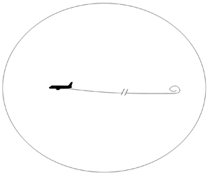
An example is the force distribution acting upon the flow by an aircraft as depicted in figure 2(a). Volume  $V_\infty$ encloses the starting vortex at a large distance from the aircraft, the trailing vortices and the bound vortex. The aircraft flies at constant speed in still air, increasing the kinetic energy in the flow domain. The velocity at the force distribution is $\boldsymbol U_0+\boldsymbol v_{st}$, with $\boldsymbol U_0$ the flying speed and $\boldsymbol v_{st}$ the velocity in a frame of reference fixed to the aircraft. In this frame $\boldsymbol f \perp \boldsymbol v_{st}$ at all surfaces of the aircraft, so the work done by the force field is $\int _{V_\infty } \boldsymbol {f} \boldsymbol {\cdot } (\boldsymbol {v}_{st} +\boldsymbol U_0)\,\textrm {d}V=\int _{V_\infty } \boldsymbol {f} \boldsymbol {\cdot } \boldsymbol {U}_0\,\textrm {d}V=D_i U_0$, where $D_i$ is the induced drag, being the component of the resultant wing load in the direction of flight.

Figure 2. Spheres as control volume  $V$ used to determine the work done by a force field distribution: (a) with the force field moving in an infinitely large volume $V_{\infty }$, (b) with a stationary force field and steady flow in a finite volume $V_{st}$, (c) with a stationary actuator disc force field and steady flow in a finite volume $V_{st}$. Only half-spheres are shown.
The force field does not perform work in the frame of reference fixed to the aircraft as then  $\boldsymbol {f} \boldsymbol {\cdot } \boldsymbol {v}_{st}=0$. Consequently, the right-hand side of (3.4) should become 0 when evaluated in the finite control volume $V_{st}$ moving with the aircraft; see figure 2(b). The flow within $V_{st}$ is steady, so the unsteady term on the right-hand side of (3.4) vanishes, by which the work done is expressed in the amount of velocity times $H$ passing the surface $S_{st}$,
 \begin{equation} \int_{V_{st}}\boldsymbol{f}\boldsymbol{\cdot} \boldsymbol{v}_{st}\,{\rm d}V =\displaystyle \int_{S_{st}}H \boldsymbol{v}\boldsymbol{\cdot} \boldsymbol{e}_{n,S}\,{\rm d}s, \quad \text{if steady flow in bounded } V_{st}. \end{equation}
The trailing vortex sheets are infinitely thin as the flow is inviscid, so the flux of  $H$ through the cross-section of the vortex sheet with $S_{st}$, is infinitely small. At all other positions of $S_{st}$ the flow is undisturbed, so the right-hand side of (3.7) is $H_0 \int \boldsymbol {v}\boldsymbol {\cdot } \boldsymbol {e}_{n,S}\,\textrm {d}s=0$ because of the continuity equation (2.2), so the right-hand side of (3.7) is $0$ indeed. This situation occurs when the aircraft is placed in a wind tunnel: the load on the model aircraft does not perform work. The aircraft generates trailing vorticity, so compared with undisturbed flow, the kinetic energy is increased, but this is balanced by lower pressures, keeping $H$ invariant. The energy put in the flow by the fan of the wind tunnel is required to balance all viscous losses of the flow when passing the aircraft, corner vanes, screens to remove turbulence, side walls and settling chamber. The actuator disc flow shown in figure 2(c) is characterised by $\boldsymbol {f} \boldsymbol {\cdot } \boldsymbol {v}\neq 0$, by which (3.7) is non-zero when using the same finite control volume $V_{st}$. The figure shows the disc flow in half of the meridian plane. The classical disc as conceived by Froude (Reference Froude1889) is a circular porous area carrying a uniform normal load $\boldsymbol F$. The disc is perpendicular to the undisturbed wind speed $\boldsymbol U_0$ in the $x$-direction. In the wake downstream of the disc $H_{wake} \neq H_0$ as the disc force field has decreased the energy content of the flow passing the disc. The decrease of energy at the disc manifests itself as a negative pressure jump across the disc, as shown in figure 3. The left part shows a smoothly decreasing velocity at the disc axis, while the right part shows an increasing pressure but with a jump at the passage of the disc.

Figure 3. The velocity  $v$ and the pressure $p$ at the axis of an actuator disc extracting energy from the flow. Here $\mathcal {F}$ is the potential of the disc force field.
4. Classification of load distributions as (non-)conservative
Whether a force field is locally conservative or not, is determined by (2.6) or (2.7). However, for a distribution as a whole, this is not a distinguishing criterion. This is illustrated by the force field  $\boldsymbol F$ acting on an aerofoil as shown in figure 1, a wing of an aircraft and an actuator disc shown in figure 2.
4.1. The load distribution on a 2-D aerofoil: conservative
With  $\boldsymbol F$ being a normal load on a closed contour, (3.2) applies. As known, a 2-D lifting body does not produce vorticity, here explained by force field considerations. However, at almost any position of the aerofoil $\boldsymbol {\nabla } \boldsymbol{\times} \boldsymbol {F}\neq 0$, by which the force field produces vorticity locally, turning the aerofoil contour to a vortex sheet. This follows by (3.1) for the steady flow $\boldsymbol {\nabla } \boldsymbol{\times} \boldsymbol {F}=\boldsymbol e_z \,\textrm {d}F/\textrm {d}s=\rho v_s \,\textrm {d}\boldsymbol \gamma /\textrm {d}s\neq 0$. When integrating $\textrm {d}F/\textrm {d}s$ along the suction side of the aerofoil, $\textrm {d}F/\textrm {d}s>0$ starting from the leading edge stagnation point up to the position of maximum $F$. This implies that $|\gamma |_{suctionside}$ increases from $0$ at the stagnation point to its maximum level when $F$ reaches its maximum. Thereafter $dF/ds<0$ towards the trailing edge, with decreasing $|\gamma |_{suction side}$. Continuation of the integration along the pressure side results in (3.2). The distribution as a whole does not produce vorticity, nor does it perform work, as at all positions of the contour $\boldsymbol F \perp \boldsymbol v$, so it is considered a conservative distribution.
4.2. The load distribution on an aircraft wing: non-conservative
Except at the symmetry line, everywhere at the aircraft wing's surface shown in figure 2,  $\boldsymbol {e}_z \boldsymbol {\cdot } (\boldsymbol {\nabla } \boldsymbol{\times} \boldsymbol {F})\neq 0$, with $\boldsymbol e_z$ the unit vector in the spanwise direction. Vorticity in the direction of the chord is generated at the surface of the wing, leaving at its trailing edge. At the same time (3.2) is valid so the integrated amount of vorticity production is $0$ as the wing generates positive and negative vorticity to the same amount. Although (3.1) applies, the distribution is considered as non-conservative. This is supported by the conclusion of § 3.2 that, in an inertial frame of reference, the load distribution performs work.
The 3-D ring wing with its axis parallel to the undisturbed flow is an exception to this. Such a ring wing or duct in perfectly aligned, axisymmetric flow does not shed vorticity in the flow. When the undisturbed flow is not parallel to the axis, the ring wing produces trailing vorticity, and becomes non-conservative.
4.3. The load distribution on an actuator disc: non-conservative
The third distribution discussed here is the actuator disc with a uniform distribution of  $\boldsymbol F$ for $r < R_{disc}$, and a jump to $0$ at $r=R_{disc}$. With (2.4) and (2.7) the load for $r < R_{disc}$ is
 \begin{equation} \boldsymbol{F}={-}\boldsymbol{e}_x \Delta \mathcal{F} = \boldsymbol{e}_x \triangle p.\end{equation}
As shown in figure 3,  $-\Delta \mathcal {F}$ lowers the pressure in the wake, in order to have undisturbed pressure far downstream. Herewith the disc force field shows two characteristics: locally $\boldsymbol F$ is the gradient of a potential, so is locally conservative, while it changes the Bernoulli parameter $H$ in the wake, indicating a non-conservative character. This is confirmed at the edge of the disc, where the load jumps from $\boldsymbol F$ to $0$, so $\boldsymbol {\nabla } \boldsymbol{\times} \boldsymbol {F}\neq 0$. Integration of (2.9) on a contour $S$ around the disc edge yields, expressed in the $x, r, \varphi$ cylindrical coordinate system,
 \begin{equation} \frac{1}{\rho} \oint_S \boldsymbol{e}_\varphi \boldsymbol{\cdot }\left(\boldsymbol{\nabla} \boldsymbol{\times} \boldsymbol{F} \right)\,{\rm d}s= \frac{1}{\rho} F= \frac{{\rm D} \gamma_\varphi}{{\rm D}t}+\frac{v_r \gamma_\varphi}{r}. \end{equation}
The term containing  $v_r \gamma _\varphi$ describes how ${\gamma}_{\varphi}$ changes when moved to another radius (van Kuik Reference van Kuik2018, § 5.5), so performs work. The distribution as a whole is non-conservative as at the disc edge $\boldsymbol {\nabla } \boldsymbol{\times} \boldsymbol {F} \neq 0$. The non-conservative force field generates vorticity at the disc edge, which forms the boundary of the wake, and performs work as in the wake $H \neq H_0$.
Equation (4.2) shows that vorticity can be produced by a force field when there is no bound vorticity to be connected to. This seems to be in contrast to the first Helmholtz theorem saying that vortex filaments can not start or end in the fluid. This is discussed in § 6.2.
The mixed characteristics of the distributions of  $\boldsymbol F$ discussed in the preceding examples, are shown in table 1. To classify distributions of forces as non-conservative, we consider the generation and convection of vorticity, disregarding its sign, as decisive. Equivalent to this is that only non-conservative force fields are able to perform work.
Table 1. Classification of the force fields of an aerofoil, wing and actuator disc.

4.4. Conservative components of load distributions
So far, only one type of a conservative load distribution is treated: the load on a 2-D lifting body. Most 3-D load distributions are non-conservative, but may have conservative components. Two examples have been analysed by van Kuik et al. (Reference van Kuik, Micallef, Herraez, van Zuijlen and Ragni2014). One is the load on chordwise bound vorticity at a rotor blade tip. The radial component of the load does not contribute to the torque, so does not perform work, but it has a small effect on the tip vortex trajectory immediately after leaving the tip (Herráez, Micallef & van Kuik Reference Herráez, Micallef and van Kuik2017). The spanwise load on bound chordwise vorticity at the wing tips is also conservative. The other example concerns the actuator disc load distribution designed to generate a Rankine vortex downstream of the disc. For the solid body rotation in the kernel of this vortex, a radial force distribution is required. A remarkable property of these conservative components of force fields is that they vanish for vanishing chord of the blade or wing, or vanishing thickness of the disc. In 3-D flows conservative loads appear as second-order loads with non-conservative loads being most important.
4.5. The effect of conservative loads
As conservative loads do not shed vorticity, they have no impact on the flow field at a large distance from the conservative distribution. At a short distance their impact is to affect pressure and velocity, or in other words: potential and kinetic energy, thereby conserving the total energy content  $H$. Using the 2-D aerofoil as an example, it is clear that far behind the aerofoil there is no trace of it left in the flow, but locally the load distribution induces the flow around the aerofoil contour.
Still conservative loads may have a larger impact when they interact with non-conservative loads. In case a rotor or fan is placed inside a ring wing or duct, the conservative load distribution at the duct lowers the pressure at the position of the rotor. The rotor, with a non-conservative load, operates in another flow state compared with the rotor without duct.
5. The Kutta–Joukowsky loads on bound vorticity in steady flow
5.1. General expression
Equation (2.3) is integrated on the volume  $V_{st}$ shown in figure 2(b). Here $V_{st}$ encloses area $A$ containing the bound vorticity $\boldsymbol \omega _A$, as well as free vorticity outside $A$, confined in infinitely thin vortex sheets, e.g. in the trailing tip vortices of a wing. As everywhere at the contour of $V_{st}$, except inside of the infinitely thin sheets, $\boldsymbol \nabla H = 0$, the left-hand side of (2.3) does not contribute to the integration. Furthermore, outside $A$ the vorticity is aligned to the flow, so the resultant load $\boldsymbol {\mathcal {R}} = \int _A \boldsymbol f \,\textrm {d}A$ is
 \begin{equation} \boldsymbol{\mathcal{R}}={-}\rho\int_A \boldsymbol{v} \boldsymbol{\times} \boldsymbol{\omega}_A \,{\rm d}A. \end{equation}
Now  $\boldsymbol v$ in (5.1) is decomposed as $\boldsymbol v=\boldsymbol e_x U_0 +\boldsymbol v_{i, b} + \boldsymbol v_{i, fr}$, with $U_0$ being the undisturbed velocity, $\boldsymbol v_{i, b}$ the velocity induced by the bound vorticity $\boldsymbol {\omega }_A$ and $\boldsymbol v_{i, fr}$ the velocity induced by free vorticity in the flow field, if present. With this decomposition it becomes
 \begin{equation} \boldsymbol{\mathcal{R}}={-}\rho\int_A \boldsymbol{e}_x U_0\boldsymbol{ \times} \boldsymbol{\omega}_A \,{\rm d}A -\rho\int_A \boldsymbol{v}_{i, b}\boldsymbol{ \times} \boldsymbol{\omega}_A \,{\rm d}A -\rho\int_A \boldsymbol{v}_{i,fr} \boldsymbol{\times} \boldsymbol{\omega}_A \,{\rm d}A. \end{equation}
In the second integral the integration area  $A$ can be replaced by $V_{st}$, as $\boldsymbol \omega _A=0$ outside $A$. Let the contour $S_{st}$ have radius $R_{st}$ and polar coordinate system $(r,\theta )$. The vector identity used to convert (2.1) to (2.3) is now used to convert this integral to an integral over the contour $S_{st}$. With the theorem of Gauss, $\int _V \boldsymbol {v}_{i,b} \boldsymbol {\times \omega }_A \,\textrm {d}V$ becomes
 \begin{equation} \int_{V} \left(\frac{1}{2} \nabla \left( \boldsymbol{v}_{i,b} \boldsymbol{\cdot} \boldsymbol{v}_{i,b}\right)-(\boldsymbol{v}_{i,b}\boldsymbol{\cdot\nabla) \boldsymbol v}_{i,b} \right)\,{\rm d}V_{st}=\oint_{S_{st}} \left(\frac{ \boldsymbol e_r}{2} \left(\boldsymbol{v}_{i,b}\boldsymbol{ \cdot v}_{i,b} \right) -\boldsymbol{v}_{i,b} (\boldsymbol{v}_{i,b} \boldsymbol{\cdot} \boldsymbol{e}_r) \right)\,{\rm d}s_{st}. \end{equation}
The first term of the integrand on the right-hand side, omitting  $\boldsymbol e_r/2$, is $\boldsymbol {v}_{i,b} \boldsymbol {\cdot } \boldsymbol {v}_{i,b}=(\boldsymbol e_r \boldsymbol v_{i,b})^2 + (\boldsymbol e_\theta \boldsymbol v_{i,b})^2$, in this paragraph abbreviated as $v_{r}^2+v_{\theta }^2$. At any position at $S_{st}$, $v_{\theta }=\varGamma / (2{\rm \pi} (R_{st}+\delta ))$ where $\delta (\theta )$ accounts for $\boldsymbol \omega _A$ being distributed within $A$ instead of concentrated at $r=0$. The order of magnitude of $\delta$ is equal to the order of largest length of $A$, so for $R_{st} \rightarrow \infty$, $\delta /R_{st} \rightarrow 0$. With this, a Taylor series development shows that
 \begin{equation} v_{\theta}^2=\left(\frac{\varGamma}{2{\rm \pi} R_{st}}\right)^2 \left(1-2\frac{\delta}{R_{st}} + 3\left( {\frac{\delta}{R_{st}}}\right)^2 - \cdots\right). \end{equation}
Consequently,  $\oint \frac {1}{2}v_{\theta }^2 \boldsymbol e_r\,\textrm {d}s \rightarrow 0$ for $R_{st} \rightarrow \infty$. As $v_r \ll v_\theta$, also $\oint \frac {1}{2}v_{r}^2 \boldsymbol e_r\,\textrm {d}s \rightarrow 0$ in this limit, as well as the second term in the integrand on the right-hand side of (5.3), since it contains $v_r^2$ and $v_\theta v_r$. Herewith (5.2) becomes
 \begin{equation} \boldsymbol{\mathcal{R}}={-}\rho\int_A \boldsymbol{e}_x U_0\boldsymbol{ \times} \boldsymbol{\omega}_A \,{\rm d}A -\rho\int_A \boldsymbol{v}_{i,fr} \boldsymbol{\times} \boldsymbol{\omega}_A \,{\rm d}A. \end{equation}
5.2. The Kutta–Joukowsky load on an aerofoil
Figure 1 shows a distribution of  $\boldsymbol F$ along a 2-D contour $S$ in the $x$–
$x$– $y$ plane, representing an aerofoil. The integral on the right-hand side of (5.5) contains only $\omega _z$, with $z$ perpendicular to the 2-D plane. There is no free vorticity, so $\boldsymbol v_{i,fr}=0$. With $\varGamma = \int _A \boldsymbol \omega \,\textrm {d}A$, the resultant load becomes the lift $\boldsymbol L$ in the well-known Kutta–Joukowsky expression,
 \begin{equation} \boldsymbol{L}={-}\rho \boldsymbol{U}_0 \boldsymbol{ \times} \boldsymbol{\varGamma}. \end{equation}
This result is most known for inviscid, steady, 2-D flows, but it can be extended to viscous, 3-D, unsteady flows as shown in Wu et al. (Reference Wu, Liu and Liu2018). As discussed in § 4.1, the load (5.6) is conservative. The Kutta–Joukowsky load is derived directly from the equation of motion (2.3). In case the body force term  $\boldsymbol f$ is not included in the Euler equation, the derivation starting from (2.10) follows a different path. Wu et al. (Reference Wu, Liu and Liu2018) have derived (5.1) by integration of the pressure on a contour enclosing the bound vorticity, where after the contour integral is converted to the volume integral (5.1). Saffman (Reference Saffman1992, § 1.9) proceeds from (2.10), but concludes in § 3.1 that an external force is necessary to balance the right-hand side of (5.1), called the vortex force. He remarks that ’if in a steady flow $\boldsymbol {v} \boldsymbol{\times} \boldsymbol {\omega }$ is not the gradient of a single-valued scalar, …, then an external non-conservative body force must be applied to maintain equilibrium’. In other words: the Kutta–Joukowsky load has to be a non-conservative load. For a 3-D lifting body like a wing, this is correct as discussed in § 4.2, but for a 2-D lifting body like an aerofoil, the Kutta–Joukowsky load is conservative.
5.3. The Kutta–Joukowsky load on a wing and its relation with the trailing vorticity
Besides spanwise bound vorticity, a wing may have bound vorticity in other directions due to the first part of the trailing vortex sheet, which is bound to the wing as indicated in the left part of figure 4. At the same time  $\boldsymbol v_i$ contains the component $\boldsymbol v_{i,fr}$ induced by the trailing vortex sheet. Usually the linearised or first-order representation of the wing plus trailing vorticity sheet, so without deformation and roll up, is used, see the right side of figure 4. Then the bound and free vorticity are assumed to be distributed in the plane $y=0$. This representation of the wake is in accordance with the vortex scheme used by Lanchester (Reference Lanchester1907) and Prandtl (Reference Prandtl1918) who have developed the lifting line theory. Modern aerodynamic textbooks still use this first-order representation of the wake (Anderson Reference Anderson2010; Chattot & Hafez Reference Chattot and Hafez2015).

Figure 4. The vortex system of a straight wing. (a) Wing with thickness, wake deformed with respect to the plane  $y=0$ (dashed lines); (b) linearised wing and wake, both in the plane $y=0$.
Using this representation of the wing and vortex sheet, the bound and free vorticity do not induce velocity in the plane  $y=0$, only perpendicular to this plane. Consequently, $\boldsymbol {v}$ consists of $\boldsymbol {e}_x U_0$ and downwash $\boldsymbol v_{i,fr}=\boldsymbol {e}_y v_y$, so (5.5) becomes
 \begin{equation} \left. \begin{array}{l} \boldsymbol{L}={-}\rho \boldsymbol{U}_0 \boldsymbol{\times} \boldsymbol{\varGamma} ,\\ \boldsymbol D_i={-}\rho \boldsymbol{\bar{v}}_y \boldsymbol{\times} \boldsymbol{\varGamma}, \end{array} \right\} \end{equation}
where  $\boldsymbol L$ is the lift, $\boldsymbol D_i$ the induced drag and $\boldsymbol {\bar {v}}_y$ the chordwise-averaged downwash.
The generation of the trailing vortex sheet is derived as follows. Again we use the linearised wake and wing model as shown in figure 4 on the right side. The  $x$-component of the curl of (2.9) is
 \begin{equation} \frac{1}{\rho} \boldsymbol{e}_x \boldsymbol{\cdot} \left( \boldsymbol{\nabla} \boldsymbol{\times} \boldsymbol{f}_y \right)= \frac{\partial f_y}{\partial z}= \left( \boldsymbol{v} \boldsymbol{\cdot} \boldsymbol{\nabla} \right) \omega_x - \left(\boldsymbol{\omega} \boldsymbol{\cdot} \boldsymbol{\nabla} \right) v_x. \end{equation}
As there is no induction in the  $x$- and $z$-directions, $\boldsymbol v = \boldsymbol U_0$ and $( \boldsymbol {\omega } \boldsymbol {\cdot } \boldsymbol {\nabla } ) v_x=0$. Integration of (5.8) across the thickness of the wing $\triangle y$ gives
 \begin{equation} \frac{1}{\rho} \frac{\partial F_y}{\partial z}= \int_{\triangle y} U_0 \frac {\partial{\omega}_x}{\partial x} {{\rm d}\kern0.05em y}=U_0 \frac {\partial{\gamma}_x}{\partial x}. \end{equation}
Equation (5.9) shows that  $\gamma _x$ increases along the chord depending on the local value of $\partial F_y / \partial z$. After integration from leading edge to trailing edge, with $L=\int F_y\,{\textrm {d} x}$, (5.9) becomes
 \begin{equation} \frac{1}{\rho U_0} \frac{\partial L}{\partial z} =\gamma_{x,te}, \end{equation}
where  $_{te}$ denotes the trailing edge of the cross-section. With (5.7) this becomes
 \begin{equation} \frac{\partial \varGamma}{\partial z}={-}\gamma_{x,te}.\end{equation}
Equation (5.10) couples the generation of the trailing vorticity to the spanwise derivative of the lift. Equation (5.11) is well known, it couples the change in bound circulation to the strength of the trailing vorticity. The lifting surface generates vorticity, but in an equal amount of opposite sign. Consequently, the integrated amount is zero, by which (3.2) is satisfied.
In § 6.2 the compatibility of these results with the theorems of Helmholtz will be discussed.
5.4. The Kutta–Joukowsky load on a vortex sheet
Equation (5.1) cannot be used as the vortex sheet may stretch to infinity, so  $A$ is not bounded. After integration of (2.3) in the normal direction, and taking the limit $\epsilon \rightarrow 0$, the left-hand side becomes a jump $\triangle H$ across the surface. The last term on the right-hand side becomes $\rho \bar {\boldsymbol {v}} \boldsymbol{\times} \boldsymbol {\gamma }$, where $\bar {\boldsymbol {v}}$ is the convective velocity of the sheet, being the average of the velocity on both sides of the vortex sheet. The result is, for $\triangle H = 0$,
 \begin{equation} \boldsymbol{F}={-}\rho\bar{\boldsymbol{v}} \boldsymbol{\times} \boldsymbol{\gamma}, \end{equation}
which is the Kutta–Joukowsky relation for the load on a vortex sheet. Alternatively, (5.12) may be derived by applying Bernoulli's equation on both sides of the vortex sheet. Every steady vortex sheet with a non-zero convective velocity carries a jump in  $H$ or a normal load $\boldsymbol F$.
5.5. The Kutta–Joukowsky load on an actuator disc
The most elementary disc proposed by Froude (Reference Froude1889) has a uniform, normal load  $\boldsymbol F$, which is not immediately recognised as a Kutta–Joukowsky load. However, the disc may be considered as the result of limit transitions for a rotor when the number of blades increases to infinity, and the rotational speed does the same (van Kuik Reference van Kuik2018, § 4.3). The load on a single rotor blade is the Kutta–Joukowsky load $-\rho \boldsymbol {v}_{rot} \boldsymbol{\times} \boldsymbol {\varGamma }$, with $\boldsymbol v_{rot}$ defined in the rotating frame of reference, and with $\varGamma$ the blade bound circulation. The result of the limit transitions is the uniform axial load $\boldsymbol F$. As in the previous section, (5.1) cannot be used directly, as in the wake of a disc $H\neq H_0$.
6. Conservative forces and potential energy, non-conservative forces and Helmholtz's theorems
6.1. Conservative forces and potential energy
The unique property of conservative forces in the Euler equation is that they do not generate vorticity which is convected with the flow. Several references consider the potential of conservative forces as potential energy, see Lamb (Reference Lamb1945, p. 8), Milne-Thomson (Reference Milne-Thomson1966, p. 30), Batchelor (Reference Batchelor1970, p. 138, 157) and Kundu (Reference Kundu1990, pp. 102–103). At the same time, some references consider pressure as potential energy (Batchelor Reference Batchelor1970, p. 157; Morrison Reference Morrison2006), so the questions are: is pressure to be considered as potential energy, and is the pressure the force potential  $\mathcal {F}$?
Equation (3.3) shows that the work performed by a force field in inviscid incompressible flow is expressed as a change of pressure and/or kinetic energy. Analogous to concepts used in rigid body mechanics it is obvious to consider pressure as potential energy. In the absence of forces the Bernoulli equation expresses conservation of energy being the sum of kinetic plus potential energy. This specifies the observation by Durand (Reference Durand1934, § I-6) and Munson, Young & Okiishi (Reference Munson, Young and Okiishi2006, § 5.3.3) who consider the Bernoulli equation as an energy conservation equation. The actuator disc example shown in figure 3 shows the exchange of potential and kinetic energy upstream and downstream of the disc, while at the disc the energy level is decreased by the jump in pressure, being potential energy. The pressure jump is minus the jump of the potential  $\mathcal {F}$, as shown by (2.8), derived for infinity thin load carrying surfaces. Consequently, pressure is potential energy and is (minus) the potential of a conservative body force field.
6.2. Non-conservative forces and the theorems of Helmholtz
The generation of vorticity by non-conservative load distributions seems to violate the first theorem of Helmholtz (Reference Helmholtz1858), which is, citing Saffman (Reference Saffman1992, § 1.5): ‘For the motion of an ideal barotropic fluid under the action of conservative external body forces  $\ldots$ fluid particles originally free of vorticity remain free of vorticity’. Indeed Helmholtz (Reference Helmholtz1858, p. 26) writes that his theorems are valid ‘if a force potential exists for all the forces acting on the fluid’. The load distribution on a 3-D lifting body, like a wing and actuator disc treated in § 5.3, is non-conservative, so the theorems are not applicable. Meyer (Reference Meyer1982, p. 42) confirms this by showing that Helmholtz's theorems do not apply to bound vorticity as the contour used to measure the bound circulation does not move with the fluid, in contrast with the contours in Helmholtz's theorems. Prandtl was aware of the obvious interpretation problem, as in Prandtl (Reference Prandtl1918, p. 16) he writes that the bound vortex does not need to satisfy Helmholtz's laws, as its position originates from the requirement to replace the lifting body. von Kármán & Burgers (Reference von Kármán and Burgers1935, § A14) say the same: ‘The adjective “bound” indicates that these vortices are kept at a fixed position in space by the action of external forces. ‘Free’ vortices on the contrary are carried along with the motion of the fluid, in accordance with Helmholtz's law’.
With Helmholtz's theorems being valid only for conservative force fields, they have nothing to do with the continuation of bound wing vorticity to trailing wake vorticity, as a wing carries a non-conservative force field. von Kármán & Burgers (Reference von Kármán and Burgers1935), Batchelor (Reference Batchelor1970), Meyer (Reference Meyer1982), Milne-Thomson (Reference Milne-Thomson1966) and Lighthill (Reference Lighthill1986) derive (5.11) using the velocity potential or applying Stokes’ theorem on a collar-shaped control surface around the bound vorticity which crosses the trailing vorticity. Prandtl & Tietjens (Reference Prandtl and Tietjens1934, § 11.1) mention that the tip vortex strength equals the bound vortex strength as shown by the criteria of the velocity potential, not by Helmholtz's laws. Also Chattot & Hafez (Reference Chattot and Hafez2015) do not use Helmholtz's theorems. The same is true for the derivation in § 5.3. Still, several textbooks do so, such as Katz & Plotkin (Reference Katz and Plotkin1991, § 4.1), Rathakrishnan (Reference Rathakrishnan2013, p. 213), Anderson (Reference Anderson2010, § 5.3), Kundu (Reference Kundu1990, § 14.9) and Branlard (Reference Branlard2017, p.89). Wu et al. (Reference Wu, Ma and Zhou2005, p. 591) mention that Prandtl and Lanchester have used Helmholtz's vorticity theorems to develop the concept of the horseshoe vortex representing a wing with trailing vortices. This is not supported by the citations of Prandtl mentioned above.
The principal difference between the flows considered by Helmholtz and the flows induced by 3-D lifting body force fields is that Helmholtz assumes only conservative forces by which vorticity is conserved, while the force fields representing 3-D lifting surfaces are non-conservative, so generate vorticity.
7. Conclusions
In the introduction two objectives were formulated: to show which force field generates or conserves vorticity and similarly converts or conserves energy, and to analyse the relation between bound and trailing vorticity expressed in force field terms. As detailed in the following, both objectives have been met.
(i) All 2-D body force distributions are conservative, so do not generate trailing vorticity nor convert energy. In 3-D flows conservative body force distributions are possible in axisymmetric flow.
(ii) All 3-D body force distributions on lifting bodies like a wing are non-conservative, generating trailing vorticity and converting energy.
(iii) Classical results like the Kutta–Joukowsky load and the relation between the trailing and bound vorticity of a wing are reproduced using the force field method. Both results follow directly from the Euler equation including the force field term.
Additional conclusions are as follows.
(i) Conservative forces do not have impact on flow properties in the far field, but still they change the near field pressure and velocity while conserving $H$.
$H$.(ii) The potential of a conservative force in inviscid, incompressible flow is (minus) the pressure. Pressure is potential energy.
(iii) Helmholtz's theorems are not applicable to couple the trailing vorticity strength to the derivative of the bound vorticity.

Acknowledgements
The author thanks A. Schaffarczyk, Kiel University of Applied Sciences, for the discussion on the ideas described in the paper, and for his suggestions and corrections. Also the three anonymous reviewers are thanked as their critical remarks have led to significant improvements as well as more accurate treatments of several details.
Declaration of interests
The author reports no conflict of interest.


 Open access