


Introduction
Glacially derived silt- and clay-sized grains influence a wide range of Earth surface processes from slope stability to chemical weathering rates. For example, the rate of silt production in the subglacial environment is thought to explain the great volume of loess deposits at a global scale (Smalley, Reference Smalley1966b; Assallay and others, Reference Assallay, Rogers, Smalley and Jefferson1998). Furthermore, the production rate and size distribution of fines are critical for controlling the deformation of till (e.g. van der Meer et al., Reference van der Meer, Menzies and Rose2003; Hart, Reference Hart2017), and thus the dynamics of the glaciers. Characterizing clay and silt from glacier systems will advance our understanding of how a large portion of these fine grains is produced at the Earth surface.
Processes of subglacial comminution
Crushing and abrasion are the two dominant processes of comminution and are assumed to occur in the following ways. Crushing occurs when compressive forces cause through-going fractures to fail in tension (e.g. Hiemstra and van der Meer, Reference Hiemstra and van der Meer1997; Hooke and Iverson, Reference Hooke and Iverson1995), predominantly exploiting gravel-sized clasts to produce sand- and silt-sized daughter grains (e.g. Haldorsen, Reference Haldorsen1981) of roughly equal size (e.g. Chaolu, Reference Chaolu1997). At the onset of comminution, crushing predominantly exploits intergranular boundaries (e.g. Haldorsen, Reference Haldorsen1981; Sharp and Gomez, Reference Sharp and Gomez1986). Abrasion results from shear forces or traction that lead to grain rounding (e.g. Hart, Reference Hart2006), predominantly acting on boulders and cobbles with minimal impact on sand-sized grains to produce silt (e.g. Boulton, Reference Boulton1978). Abrasion is thought to be required to exploit intragranular fractures (e.g. Haldorsen, Reference Haldorsen1981). Subglacial abrasion has been argued to produce grains that are predominately silt-sized, the so-called ‘terminal grade’ of Dreimanis and Vagners (Reference Dreimanis, Vagners and Goldthwait1971). The exact size of the terminal grade depends on lithology (Dreimanis and Vagners, Reference Dreimanis, Vagners and Goldthwait1971; Haldorsen, Reference Haldorsen1981), but is thought to be no smaller than 1 μm (e.g. Meyer et al., Reference Meyer, Downey and Rempel2018; Lipovsky and others, Reference Lipovsky2019). As such, clay-sized grains are assumed to be sourced from clay minerals within the bedrock (e.g. Haldorsen, Reference Haldorsen1983). Within this framework, comminution is described as being discrete, i.e. crushing and abrasion selectively exploit different grain-size modes to produce distinct daughter-size populations no smaller than silt (see Fig. 6 in Haldorsen, Reference Haldorsen1981).
Observations from other workers indicate that there is no clear boundary between crushing and abrasion processes (e.g. Rogers et al., Reference Rogers, Krueger and Krog1963; Chaolu, Reference Chaolu1997; Langroudi and others, Reference Langroudi, Jefferson, Ohara-Dhand and Smalley2014). The observation of rounded sand-sized quartz grains (e.g. Hart, Reference Hart2006; Rose and Hart, Reference Rose and Hart2008; Altuhafi and Baudet, Reference Altuhafi and Baudet2011) also challenges the aspects of the discrete-comminution model because it shows that grain rounding can operate continuously across a range of sizes. Furthermore, tangential stresses normally associated with abrasion can result in ring and meridional cracks (e.g. Hiemstra and van der Meer, Reference Hiemstra and van der Meer1997) that can increase roughness, rather than promote rounding. In contradiction to a silt-size comminution limit, Langroudi and others (Reference Langroudi, Jefferson, Ohara-Dhand and Smalley2014) show that grains can evolve to ever-smaller sizes with time-dependent stresses that promote fatigue fracture (e.g. Moss, Reference Moss1966). Theoretically, the plastic limit of silicate minerals should result in grain sizes well below the assumed minimum size of 1 μm (Sammis and Ben-Zion, Reference Sammis and Ben-Zion2008). Sub-micrometre-sized grains have been observed in many SEM studies of till (e.g. Chanudet and Fillela, Reference Chanudet and Fillela2006; Rose and Hart, Reference Rose and Hart2008), even in areas where the bedrock does not contain clay minerals (Altuhafi and Baudet, Reference Altuhafi and Baudet2011). These observations support a continuous-comminution model, whereby crushing and abrasion overlap across a wide range of sizes that continue into the finest grain size.
The probability of fracturing a grain depends on the grain's internal properties, such as mineral species, size and orientation (e.g. Tavares and das Neves, Reference Tavares and das Neves2008), grain shape (e.g. Bjørk et al., Reference Bjørk, Mair and Austrheim2009; Ma and others, Reference Ma, Zhou, Regueiro, Wang and Chang2017) and microfracture length (e.g. Sharp and Gomez, Reference Sharp and Gomez1986) and density. The probability of fracture also depends on external factors such as the rate, direction and magnitude of applied stress (e.g. Sammis and Ben-Zion, Reference Sammis and Ben-Zion2008; Langroudi and others, Reference Langroudi, Jefferson, Ohara-Dhand and Smalley2014). Glaciological factors include the transport distance of till (e.g. Dreimanis and Vagners, Reference Dreimanis, Vagners and Goldthwait1971; Altuhafi and Baudet, Reference Altuhafi and Baudet2011) and the subglacial-cavity size within which clasts can be crushed (e.g. Boulton, Reference Boulton1978). Internal and external factors often compete to determine how susceptible till is to grinding. For example, at the onset of comminution, relatively large grains fracture easily because they contain large microfractures, but at later stages, large grains are stabilized by the cushioning of smaller grains, thereby decreasing the concentration of force (e.g. Iverson et al., Reference Iverson, Hooyer and Hooke1996). The cushioning effect should result in a fractal distribution of grain sizes (e.g. Hooke and Iverson, Reference Hooke and Iverson1995; Iverson et al., Reference Iverson, Hooyer and Hooke1996), leading to the interpretation that the process and extent of comminution dictate the grain-size distribution.
The relative rates of abrasion versus crushing are thought to depend on grain size, and can lead to distinct grain-size distributions, such as fractal (e.g. Hooke and Iverson, Reference Hooke and Iverson1995; Iverson et al., Reference Iverson, Hooyer and Hooke1996), log-normal (e.g. Buller and McManus, Reference Buller and McManus1973; Haldorsen, Reference Haldorsen1981) or multimodal (e.g. Dreimanis and Vagners, Reference Dreimanis, Vagners and Goldthwait1971; Haldorsen, Reference Haldorsen1981; Sharp and others, Reference Sharp, Jouzel, Hubbard and Lawson1994; Benn and Gemmell, Reference Benn and Gemmell2002). The resulting grain size of the comminuted material also depends on the microfracture density (e.g. Langroudi and others, Reference Langroudi, Jefferson, Ohara-Dhand and Smalley2014) and mineral hardness (e.g. Dreimanis and Vagners, Reference Dreimanis, Vagners and Goldthwait1971; Haldorsen, Reference Haldorsen1981; Chaolu, Reference Chaolu1997), and thus rock type (e.g. Smalley, Reference Smalley1966b; Mills, Reference Mills1977; Cammeraat and Rappol, Reference Cammeraat and Rappol1987). The influence of source-rock properties versus comminution processes in controlling grain characteristics remains unclear.
The role and origin of microfractures
Grain-size reduction occurs by brittle fracture via crack-tip propagation (e.g. Sharp and Gomez, Reference Sharp and Gomez1986; Hiemstra and van der Meer, Reference Hiemstra and van der Meer1997), with additional microfractures developing through subcritical crack growth (e.g. Haldorsen, Reference Haldorsen1981; Atkinson, Reference Atkinson1984; Sharp and Gomez, Reference Sharp and Gomez1986). At the scale of our investigation, fracture occurs along μm–mm scale microfractures. The microfractures relevant to the fracture of silt-sized grains can be intragranular (within a mineral) or intergranular (at the contact between minerals). Intragranular fractures occur along planar weaknesses, often following crystallographic orientation. Weaknesses include cleavage planes, inclusions and other impurities, exsolution lamellae, twinning and subgrain boundaries (e.g. Drewry, Reference Drewry1986; Lawn, Reference Lawn1993; Klein and Dutrow, Reference Klein and Dutrow2007). Microfractures vary amongst minerals, from twinning planes that follow crystal structure in feldspars, to imperfect cleavage that leads to conchoidal fracture in quartz.
Quartz grains in plutonic rocks can develop a characteristic silt-sized fracture spacing as the rock cools (Smalley, Reference Smalley1966a; Moss and Green, Reference Moss and Green1975), leading to the production of silt from sand-sized quartz grains (e.g. Smalley, Reference Smalley1966b). Sedimentary grains can be largely free of microfractures because they have been recycled, causing polycrystalline or deformed quartz grains to be broken down to smaller sizes (Haldorsen, Reference Haldorsen1981; Wright, Reference Wright1995; Langroudi and others, Reference Langroudi, Jefferson, Ohara-Dhand and Smalley2014). Metamorphic reactions can result in an overprinting of fresh microfractures (Slatt and Eyles, Reference Slatt and Eyles1981) and the development of polycrystalline quartz (Gomez et al., Reference Gomez, Dowdeswell and Sharp1988; Mazzullo and Ritter, Reference Mazzullo and Ritter1991). Alternatively, annealing can lead to a reduction in planar defects and dislocation density during metamorphism. While the microfracture density depends specifically on the rock type, the density has been found to correlate with the distance and displacement of proximal fault systems (e.g. Anders and Wiltschko, Reference Anders and Wiltschko1994; Faulkner and others, Reference Faulkner, Mitchell, Healy and Heap2006). The distribution of microfracture length can be fractal (e.g. Anders et al., Reference Anders, Laubach and Scholz2014). Measurements of fracture spacing, however, are much more limited. A log-normal microfracture spacing has been observed in sandstone by Hooker et al. (Reference Hooker, Laubach and Marrett2018), who suggest that spacing can evolve from exponential to log-normal.
Overarching objectives and specific research questions
In this work we analyse the mineralogy and microstructure of grains smaller than medium silt that were collected from suspension in proglacial streams, and compare this to the bedrock properties from which the sediment was derived. Within this size range, we seek to understand (i) the relative influence of source-rock properties versus subglacial comminution processes in controlling sediment characteristics and (ii) whether a continuous- or discrete-comminution model best explains the characteristics of glacially derived silt and clay. To address these overarching research objectives, we pose the following three research questions: (1) What is the grain-size distribution of fines? (2) What is the relative abundance of inter- versus intragranular fractures? (3) Do silt and clay grains undergo changes in shape and rounding when subject to abrasion? In each question, we investigate the influence of grain mineralogy. In (1) we investigate the role of bedrock lithology, in (3) we investigate the influence of grain size and in (2) we investigate both.
Field area
We collected samples from 20 glacierized basins in the Donjek Range and Maxwell Group of the St. Elias Mountains, Yukon, Canada (Fig. 1). Bedrock samples were collected from outcrops at the margins of the glaciers and suspended sediment samples from each of the proglacial streams.

Fig. 1. Study area within the St. Elias Mountains, Yukon, Canada. Circles indicate proglacial stream sampling locations where suspended sediments were collected. Squares indicate bedrock outcrop locations at the margin of the glaciers where rock samples were collected. Squares are colour coded by rock-type (plutonic or metasedimentary) and circles are coded as basin lithology (metasedimentary or mixed-lithology). Glaciers numbered 1–20 are colour coded by surge-type (red) and non-surge-type (blue). Bedrock geology compiled by Gordey and Makepeace (Reference Gordey and Makepeace1999). Landsat 7 imagery as background.
Lithology and mineralogy
Of the 20 unnamed glaciers (referred to as Glaciers 1–20), 11 are underlain by metasedimentary rock, while eight are underlain by metasedimentary rock at lower elevations and felsic plutonic rock at higher elevations. Glacier 1 is unique in that it is underlain solely by felsic plutonic rock (Crompton and others, Reference Crompton, Flowers, Kirste, Hagedorn and Sharp2015). A whole-rock chemical digest shows that the plutonic rocks range in $\rm SiO_2$ content from 66 to 70% (granodiorite to granite), and thin sections show that the grain size of the plutonic rocks is ~ 1000 μm. All metasedimentary rocks are fine-grained (~ 100 μm) and have been subject to biotite-grade metamorphism (Campbell and Dodds, Reference Campbell and Dodds1978) in the greenschist facies, with well-developed crenulation cleavage and schistosity (Fig. 2). The metasedimentary rocks show a wide range of compositions, but can be generally described as calcareous pelites with an average composition of quartz, calcite and/or dolomite, plagioclase, muscovite and biotite. Within the metasedimentary unit, which belongs to the Kaskawulsh group of the Alexader terrane (e.g. Israel and Cobbett, Reference Israel, Cobbett, Emond, Bradshaw, Lewis and Weston2008), rocks have been mapped as phyllite, siltstone, greywacke, basalt, andesite and limestone (Campbell and Dodds, Reference Campbell and Dodds1978; Dodds and Campbell, Reference Dodds and Campbell1988; Wheeler, Reference Wheeler1963), though we observe no volcanic or purely carbonate rocks at the outcrops that we sampled. For all rock fragments and sediment samples, the main alteration products are chlorite and illite and/or smectite. In this work, we focus our analysis on physical erosion of the primary minerals quartz and plagioclase (tectosilicates), muscovite and biotite (phyllosilicates) and carbonate (includes calcite, dolomite and ankerite-dolomite). The muscovite is undifferentiated white mica. See Appendix A for description of compositional bins.

Fig. 2. Thin section images of rock samples. (a) Granodiorite (plutonic) rock from Glacier 1 at 2X magnification in cross-polarized light showing (1) a transgranular microfracture spanning minerals of different phases, (2) a transgranular microfracture that cross cuts the boundary between quartz and biotite, terminating in the centre of both grains, (3) an intragranular microfracture cutting through polycrystalline quartz and (4) an intragranular microfracture that aligns with the direction of cleavage for biotite. (b) Granodiorite rock from Glacier 20 rock at 2X magnification in cross-polarized light with (1) transgranular microfractures that cut the boundary of quartz and plagioclase and (2) an intragranular fracture that truncates at the boundary between quartz and plagioclase. (c) Metasedimentary rock from Glacier 10 at 10X magnification in cross-polarized light showing biotite foliation separated by a matrix of quartz, calcite, dolomite, feldspar and micas. (d) Metasedimentary rock at Glacier 14 at 10X magnification in plane-polarized light showing micas with complex structures of microfractures. Note that the entire size distribution of the grains analysed in this work fit within a typical grain of mica.
Regional geology
The metasedimentary rock is Paleozoic in age and underwent one stage of ductile deformation prior to the intrusion of the Jurassic to Cretaceous aged felsic plutonic rock (Campbell and Dodds, Reference Campbell and Dodds1978; Israel and Cobbett, Reference Israel, Cobbett, Emond, Bradshaw, Lewis and Weston2008). A second phase of pre-Cenozoic ductile deformation was later overprinted by a post-Miocene brittle deformation event that is coincident with the rapid rise of the St. Elias Mountains and the onset of glaciation (Cobbett and others, Reference Cobbett, Israel, Mortensen, Joyce and Crowley2017; Eisbacher and Hopkins, Reference Eisbacher and Hopkins1977). Though rocks in this area show a high intact strength based on simple hammer tests, brittle damage has resulted in a relatively high degree of jointing, with a log-normal bedrock fracture spacing and a mean spacing on the order of 0.1 m (Crompton et al., Reference Crompton, Flowers and Stead2018). Exhumation rates are currently low at 0.1–0.5 mm a−1 (Dodds and Campbell, Reference Dodds and Campbell1988; Enkelmann and others, Reference Enkelmann, Piestrzeniewicz, Falkowski, Stübner and Ehlers2017), despite active exhumation (5 mm a−1) in the coastal and Southern St. Elias Mountains (Berger and others, Reference Berger2008; O'Sullivan et al., Reference O'Sullivan, Plafker and Murphy1997; Enkelmann and others, Reference Enkelmann, Piestrzeniewicz, Falkowski, Stübner and Ehlers2017), and present day activity along Denali and Duke River Faults to the north (Cobbett and others, Reference Cobbett, Israel, Mortensen, Joyce and Crowley2017; Marechal and others, Reference Marechal, Mazzotti, Elliott, Freymueller and Schmidt2015).
Glacier characteristics
Glaciers 1 and 2 have an equilibrium line altitude of ~ 2550 m above sea level (MacDougall et al., Reference MacDougall, Wheler and Flowers2011). They are known to be polythermal, with temperate ice in the accumulation area that grades into cold ice in the ablation area (Wilson et al., Reference Wilson, Flowers and Mingo2013). The modelling of Wilson and Flowers (Reference Wilson and Flowers2013) suggests that all similarly sized glaciers in this area are likely to share broadly similar thermal structures. The study glaciers range in length from 2.6 to 7.8 km ($\bar {l}=5.1$ km) and slope from 5.4 to 17.3° ($\bar {\theta }=9.1^{\circ }$
 ). Ice-penetrating radar data show that Glaciers 1–3 have depths on the order of 100 m, amounting to an overburden of ~1 MPa, which is two orders of magnitude lower than the compressive strength of a typical granite. A continuous till cover is observed at the terminus of all glaciers. Eleven of the glaciers are surge-type and the remaining nine are non-surge-type.
Methods
Sample collection and processing
We collected suspended sediment samples from the turbulent proglacial streams at each glacier. Samples were collected by raising and lowering a bottle throughout the depth of the stream. We also analysed one sediment sample collected from the bottom of a borehole drilled to the bed of Glacier 1. A downhole camera showed that sediments were sampled from a till or sediment layer. At 17 of the glaciers, we collected till to quantify the fraction of sub-sand-sized material, but fines from the till were not further analysed. Till samples were collected from exposed cutbanks that were proximal to or beneath the ice at the terminus.
To avoid flocculation (e.g. Woodward and others, Reference Woodward, Porter, Lowe, Walling and Evans2002), sediments were dispersed using 0.05% sodium hexametaphosphate solution. Samples were then dried, weighed for concentration and sieved below 90 μm. The grain-size distributions of the suspended sediments were determined up to 90 μm using a laser particle-size analyser (Crompton and Flowers, Reference Crompton and Flowers2016), but for this study we focus on the grain size of the sub-25 μm fraction. We take 4 μm to be the boundary between silt and clay and when plotting grain sizes we use the natural log.
With the exception of Glaciers 3 and 12, we collected one or two rock samples from outcrops at the margins of each glacier. Rock samples were cut with a rock saw, which removed variable amounts of weathering rind. The cut rock samples were fragmented using electrical pulse disaggregation (EPD) at Queen's University. The rock samples were placed in water and subjected to electrical discharges of up to 200 kV, but the number of pulses was not recorded. During EPD, grains are liberated by electrical breakdown and electrostrictional tension. For the latter, plasma that is channelled through a connected network of microfractures expands and explodes to form an interfering set of shock waves that disaggregate the rock as the outward force exceeds the tensile strength at a discontinuity (e.g. Andres et al., Reference Andres, Jirestig and Timoshkin1999; Giese and others, Reference Giese2010). Fracture also depends on the contrast in electrical permittivity of the material on either side of a discontinuity, and the curvature and orientation of the discontinuity relative to the direction of applied voltage (Wang and others, 2012). Many of the rocks contained larger clasts that escaped fragmentation, but the small number of coarse grains did not allow for a statistically meaningful comparison across samples. For this reason, we limited our analysis to the sub-25 μm fraction. Fines produced through EPD were processed and analysed using the same procedures as the suspended sediment.
Automated mineralogy
Samples were analysed at SGS, Burnaby, Canada using QEMSCAN®, which is an automated scanning electron microscope that exploits X-ray and backscatter electron signals to analyse elemental composition and generate a map of the inferred mineralogy (e.g. Gottlieb and others, Reference Gottlieb2000; Beckingham and others, Reference Beckingham2016). Over 6 × 10⁵ grains with 38 compositional mineral bins were analysed at a pixel-size resolution of 0.66 μm (examples shown in Fig. 3). Grains were mounted and randomly oriented in a polished resin, and results are given as 2-D projections of the grain surfaces. To avoid a grain-size bias close to the detection limit, we omit the smallest single-pixel grain size when computing size distributions. Automated mineralogy results are further constrained by X-ray diffraction (for sediment only and Glacier 1 rock), thin section analysis (for rock only, see Fig. 2) and bulk chemical digest for all samples. SEM images were obtained for Glacier 1 sediment (Fig. 4), but were not used for micromorphological analysis.

Fig. 3. Visual example of grain analysis output. (a) Sediment derived from plutonic rock at Glacier 1. (b) Sediment derived from metasedimentary rock at Glacier 5. These images only show a portion of the sample for the largest grains, but show all mineral phases that were analysed.
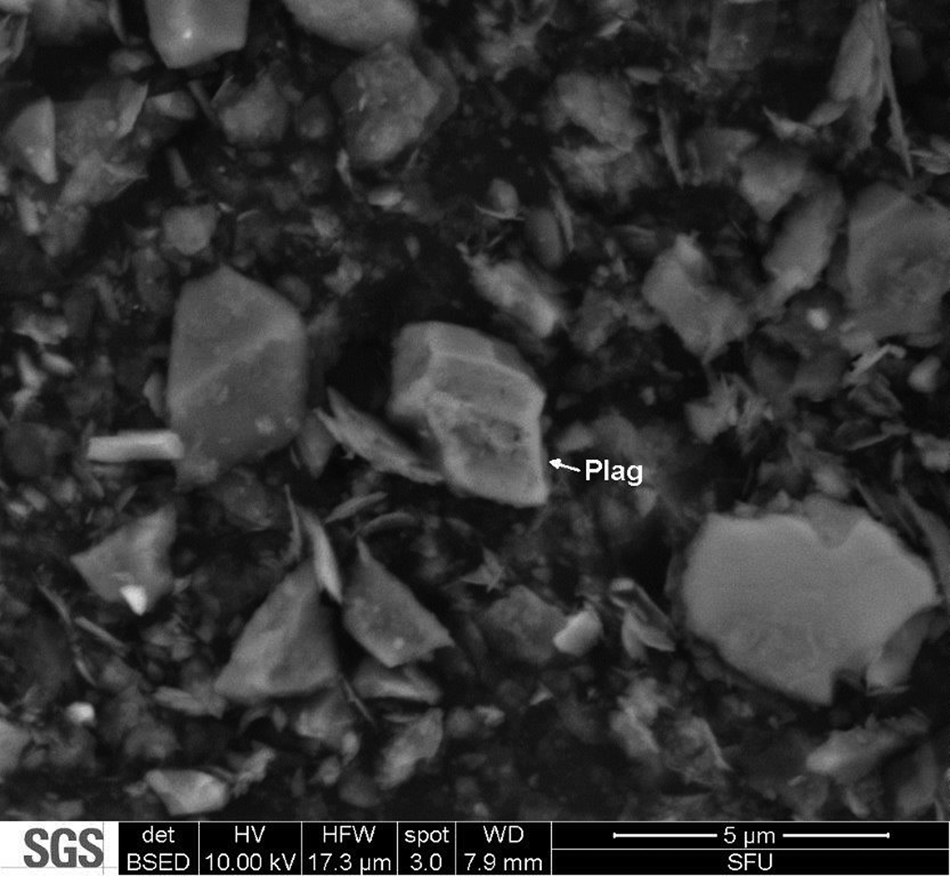
Fig. 4. Scanning electron microscope (SEM) image of sediment grains from the proglacial stream of Glacier 1. Numerous grains below the 0.66 μm detection limit for QEMSCAN can be seen. Potential edge rounding is shown on a grain of plagioclase (arrow).
Metrics for quantifying grain characteristics
We developed an algorithm in Matlab similar to the Hoshen–Kopelman algorithm to isolate grains and clusters of minerals within rasterized images. The data and code can be downloaded from Github at https://github.com/jwheelsc/grain_sorting.
Various metrics (described below and in Appendix B) are used to test for differences between groups of rock fragment samples and sediment samples (see Appendix C for full description of statistical methods). The four groups that we use are metasedimentary rocks (n = 20), plutonic rocks (n = 4), metasedimentary sediments (n = 11) and mixed-lithology sediments (n = 9, including the Glacier 1 endmember). To determine whether a difference is statistically significant between groups for a given sample statistic, we use the Tukey-HSD test at α = 0.05. The Tukey-HSD test is carried out on the means of two groups as a test of independent means, and by comparing differences in sediment and rock fragments collected from the same basin using a pairwise-comparison test (e.g. Snedecor and Cochran, Reference Snedecor and Cochran1989). In addition, when comparing across an entire distribution of sizes, we lump together all grains of the same sample type (e.g. metasedimentary rock samples) to increase the number of grains in a size class. We also carry out principal component analysis on metrics that are computed within discrete grain-size bins.
The following metrics are used to address the three research questions using the automated mineralogy data (see Appendix B for mathematical description).
1. We start by analysing the grain-size distribution (f(D i)). The subscript i denotes the size class of grain diameter D. As an attempt to understand the underlying controls on f(D i), we introduce the mineral-size distribution ($N^c_j\lpar D_k\rpar$
 ), representing the distribution of mineral clusters within grains of all sizes, and the embedded distribution ($N^d_{j\comma k}\lpar D_i\rpar$), representing the distribution of mineral-cluster sizes within grains of known size. The subscript k denotes the size class of the mineral cluster of size D for the j th mineral. To understand how minerals concentrate at different grain sizes relative to each other, we analyse the fraction of a mineral area relative to the area of all minerals within a given grain-size class (ψ j(D i)). To characterize the preferred daughter size for each mineral, we analyse the mineral-area distribution, whereby the area is only considered for the mineral of interest ($f^A_j\lpar D_i\rpar$). To understand the difference in area distributions between rocks and sediment, we model the addition/removal of material derived from abrasion (see below) to the grain-size distribution of the rock fragments, then calculate the resulting hypothetical sediment-size distribution.
2. To investigate the relative abundance of intra- versus intergranular contacts, we analyse the homogeneity of grains ($\bar {h}_j\lpar D_i\rpar$
), representing the fraction of a given mineral within a grain of a given size, averaged over all grains. We also analyse the distribution of contact lengths ($\Gamma _{j\comma g_A}\lpar n_p\rpar$). Contacts can occur between pixels of the same mineral, pixels of a given mineral at the edge of a grain or neighbouring pixels of different minerals. For intra- and intergranular contacts, the discrete length of pixel contacts is computed for each grain and normalized by the total contact length of the mineral of interest within the sample. By analysing the normalized contact length, we can determine the likelihood of inter- versus intragranular contacts for a given contact length. By analysing the difference in normalized contact lengths between rock fragments and sediments, we can quantify the difference in abundance of inter- versus intragranular fractures. By comparing the contact lengths for sediment derived from different rock types, we can get a sense of how the rock type affects inter- versus intragranular contact lengths.3. To quantify the grain shape we compute the aspect ratio. To quantify the change in roughness, we analyse the difference in the perimeter of the convex hull between rock fragments and sediment for a given grain size and mineral. We also perform a Fourier shape analysis (see Supplementary Material section 1).


Results
What is the grain-size distribution of fines?
Size distribution as a function of lithology
Thin sections show that the crystal size in the plutonic rock (~ 1000 μm) is much larger than in the metasedimentary rock (~ 100 μm). Despite the wildly different crystal sizes, rock fragments and sediments derived from both rock types have a fairly similar size distribution (Fig. 5a). For both lithologies, rock fragments and sediments are significantly smaller than the mineral size observed in thin section, indicating that the spacing of microfractures being exploited is much less than the mineral size. The mode of the distribution occurs at the smallest grain size for both rock fragments and sediment (Figs 5a and b), indicating that electrical and subglacial comminution likely produce grains smaller than the 0.66 μm detection limit.
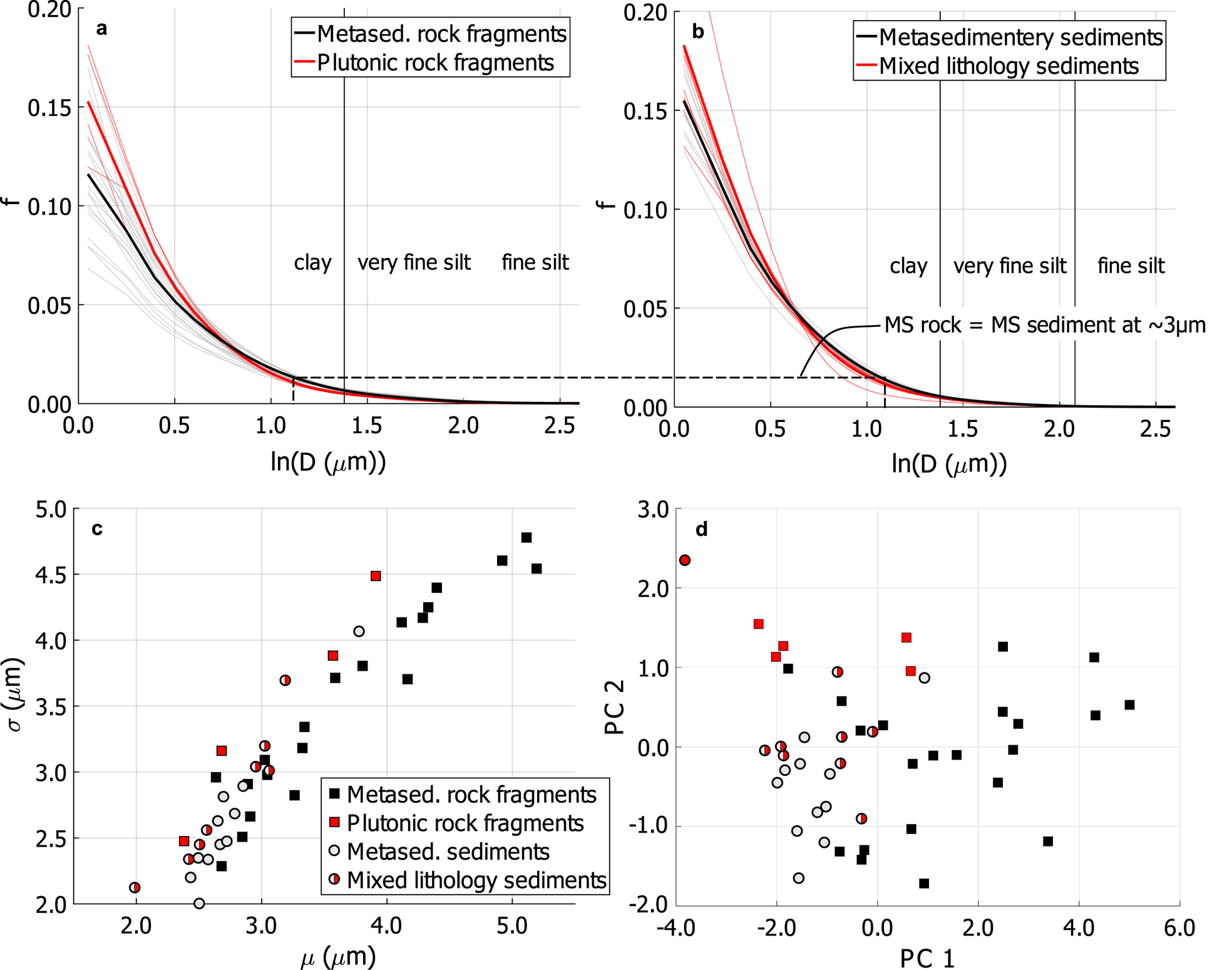
Fig. 5. Frequency distribution f(D i) of EPD rock fragments and glacial sediment. (a) Log-normal fits to the distributions of samples from plutonic rock fragments (thin red lines) and metasedimentary rock fragments (thin black lines). Thicker lines show the average size distribution by combining grains from all samples of a given type. (b) As in (a) but for metasedimentary sediments in grey and mixed lithology sediment in red. The dashed black line connecting the metasedimentary rock fragments and sediments shows the ~ 3 μm intersection point between the two. (c) Sample statistics (mean and standard deviation) for all samples, with rock fragments as squares and sediment samples as circles, colour coded by rock type and basin lithology. (d) Principal component 1 and 2 scores using all samples, with sample coding as in (c).
Despite the similarities in the range of grain sizes, plutonic and metasedimentary rock fragments show differences in their grain-size distributions. Plutonic rock fragments have a greater abundance of the smallest grains and a larger ratio of standard deviation to mean grain size (Figs 5a–c). When analysing all samples together, plutonic rock fragments are differentiated from the metasedimentary rock fragments by the first and second principal components (Fig. 5d). The second principal component can also separate mixed-lithology sediment from metasedimentary sediment.
Grain- and mineral-size distributions
For both lithologies, and for both sediment and rock fragments, the grain- and mineral-size distributions are best fit by log-normal functions (see Fig. 6). The Weibull and exponential distributions also fit well (R 2 > 0.9), while the power-law distribution does not. Although the log-normal distribution is the best fit, a slight bimodality of the distribution appears around ~ 5 μm for most minerals, which is more pronounced in the rock than in the sediment.
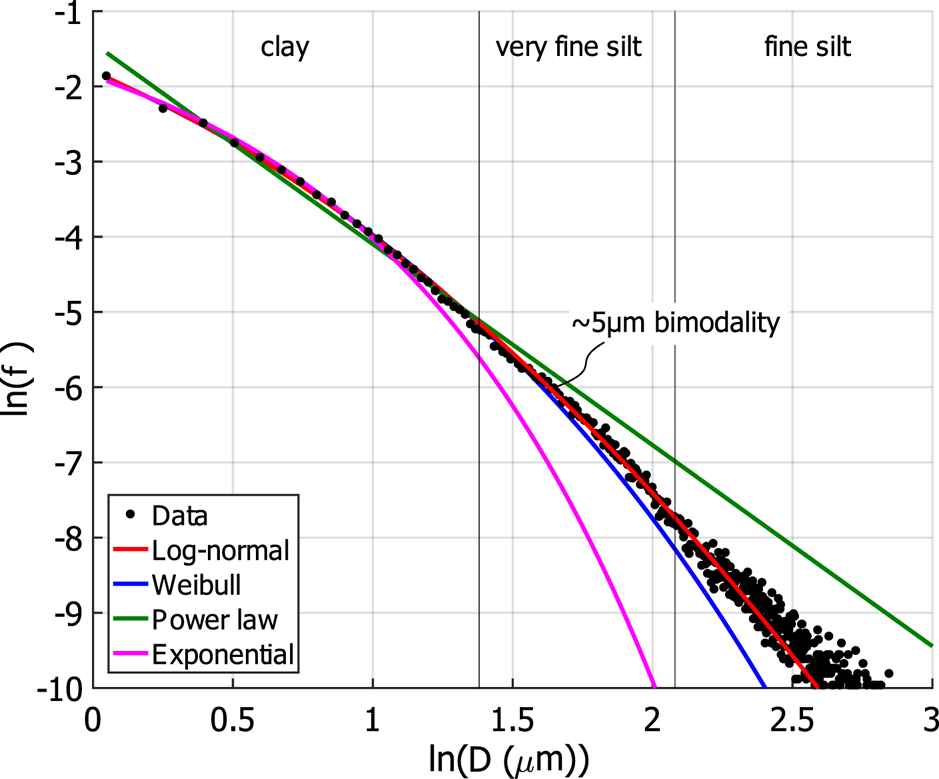
Fig. 6. Various fits to the size distribution of all metasedimentary sediment, with red line in this figure equivalent to thick black line in Figure 5b. Each point is the frequency of the i th size, with the frequency plotted in log–log space to highlight the theoretical distributions that under or overestimate the tail of the size distribution at large grains.
We use the embedded distribution $N^d_{j\comma k}\lpar D_i\rpar$ to further investigate the reasons for log-normality in both the grain- and mineral-size distributions. For both rock fragments and sediment, the embedded distribution is best fit with a two-term log-Gaussian for all minerals (see Supplementary Material section 2). The first term peaks at mineral sizes that are close to the grain size (monomineralic). The second term is much lower in amplitude than the first term, and shows how small clusters of minerals are embedded in grains of much larger sizes, which should have an influence on the distribution of stress within a grain.
Differences between sediment and rock fragments derived from the metasedimentary rocks
In comparing the metasedimentary sediments to the metasedimentary rock fragments, the sediments have a lower mean grain size and a greater abundance of grains less than ~ 3 μm (dashed line in Figs 5a and b). Across all metasedimentary samples, an analysis of the mineral-size distributions ($N^c_j\lpar D_k\rpar$ ) shows a statistically significant decrease in the mean mineral size from rock to sediment for calcite, biotite and muscovite, but not for quartz or plagioclase. By lumping grains from all samples together, all minerals show a greater abundance of mineral sizes less than ~ 3 μm in sediment than rock fragments (Fig. 7a), consistent with the results from the full grain-size distribution. The difference between plutonic rocks and mixed-lithology sediments is not discussed because grain-size reduction processes cannot be separated from mixing of rock types in mixed-lithology basins.

Fig. 7. Analysis of mineral size and area using grains from all metasedimentary sediment samples or all rock samples combined. Distributions are smoothed using spline estimates. (a) Difference in mineral-size distributions ($N^c_j\lpar D_k\rpar$ ) between sediment and rock fragments. A higher abundance of mineral clusters occurs in sediment below ~ 3 μm. (b) Mineral-area distribution ($f_j^A\lpar D_i\rpar$
 ) for sediment samples (solid lines) and rock fragments (dashed lines). Squares plotted at the mode of the distribution are plotted against the Mohs-scale hardness in inset. Mohs hardness values are taken from Klein and Dutrow (Reference Klein and Dutrow2007), with horizontal bars indicating the range in hardness values based on compositional variation with a mineral grouping (e.g. calcite and dolomite within carbonate). (c) Mineral abundance as a function of grain size (ψ j(D i)) for sediment samples and (d) the difference in ψ j(D i) between sediment (superscript s) and rock fragments (superscript r).
Area-per cent mineralogy of clay- and silt-sized grains
For both the rock fragments and the sediment, the mineral-area distribution ($f^A_j\lpar D_i\rpar$ ) shows that the abundance of clay-sized grains is highest for muscovite, followed by biotite, carbonate, plagioclase and quartz (Fig. 7b), as is the case for the frequency-based $N^c_j\lpar D_k\rpar$
 distribution. Quartz shows the highest relative abundance at the largest grain size. The frequency at the mode of the distribution is inversely correlated with the Mohs-scale hardness of the mineral (R 2 = 0.96, inset in Fig. 7b). The extent of size reduction is therefore highly correlated with the hardness of the mineral for sediment (solid lines, Fig. 7b). For the rock fragments, however, the correlation is weak (R 2 = 0.46, dashed lines, Fig. 7b). Like the mineral-size distributions, the area distributions of rock fragments and sediments are also weakly bimodal with a second peak at ~ 5 μm. In sediment compared to rock fragments, all minerals show a decrease in mean size for which the mineral area is concentrated. Only the largest differences are statistically significant (biotite and muscovite), while quartz has the smallest difference.
By analysing the abundance of a mineral relative to all other minerals within a given grain-size class (ψ j(D i)), we see that quartz makes up most of the mineral area for the largest observed grain sizes, while muscovite dominates the clay-sized fraction (Fig. 7c). In comparison to the rock fragments, quartz and plagioclase are enriched in sediment across all grain sizes, while calcite, biotite and muscovite are depleted (Fig. 7d). The same conclusions can be drawn from a pairwise-comparison of sample statistics, but the differences are only significant for plagioclase and quartz. We infer that all minerals are being crushed below the detection limit, but probably to a greater extent for the phyllosilicate and carbonate minerals, thereby causing an apparent enrichment of quartz and plagioclase in sediment relative to rock.
From the ψ j(D i) distribution, we can calculate the fractions of clay-sized grains that are composed of comminuted primary minerals versus clay minerals (defined compositionally) of the same size. In sediment, we observe that roughly 60% of clay-sized grains are composed of the primary minerals quartz, plagioclase, carbonate, biotite and muscovite. The bulk of the remaining area per cent can be accounted for by the clay minerals kaolinite, illite/smectite, chlorite, talc and vermiculite (zeolite group).
What are the relative rates of inter- and intragranular fracture?
The mean of the mineral-size distribution ($N^c_j\lpar D_k\rpar$ ) decreases from rock fragments to sediment for all minerals, indicating enhanced intragranular fracture for sediment. The observed mineral-size reduction cannot fully explain the difference in grain-size distributions between rock fragments and sediment, therefore intergranular fracture must also be taking place. The mineral size in rock, and the relative extents of inter- versus intragranular fracture, dictates the grain homogeneity and can be characterized by the normalized distribution of contact lengths.
Mean grain homogeneity
We observe a mean homogeneity of > 90% for the smallest grain sizes, and increasing heterogeneity with size (Fig. 8). Though the mean is high for the smallest grain size, we see a wide range in homogeneity and a significant fraction of multimineralic grains. As confirmed by the low ratio of amplitudes between the first and second term of the embedded distribution, plagioclase shows the lowest homogeneity at small sizes. The homogeneity of sheet silicates and carbonates decrease strongly with grain size, while that of the tectosilicates does not.
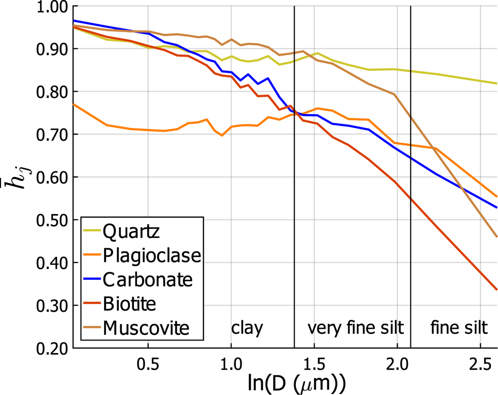
Fig. 8. Mean homogeneity $\bar {h}_j$ of all metasedimentary sediment grains for all minerals.
For all minerals, the sediments are more homogeneous than the rock fragments, except at the very largest grain sizes. For quartz, sediments have a greater mean homogeneity than rock fragments across all sizes. Metasedimentary sediments are more homogeneous than mixed-lithology sediments across all sizes, with calcite showing the greatest difference in homogeneity. An exception is for biotite, where isolated flakes of biotite are more common in mixed-lithology sediment than metasedimentary sediment.
Normalized inter- and intragranular contact lengths
For both rock and sediment, quartz exhibits the lowest normalized number of intergranular contacts with all other minerals ($\Gamma _{j\comma g_{A}}\lpar n_p\rpar$ , Fig. 9a). Within rock fragments, and in increasing order, carbonate, plagioclase, biotite and muscovite show a higher normalized number of contact lengths with other minerals. The order is slightly different for sediment, increasing from plagioclase to carbonate to biotite (depending on the contact length within a grain), to muscovite. Carbonate shows the greatest difference in intergranular contact lengths ($\Gamma _{j\comma g_A}\lpar n_p\rpar$
 ) between rock and sediment, followed by biotite, muscovite, plagioclase then quartz, with slight variations in order that depend on size (Fig. 9a). In general, the difference in the distribution of $\Gamma _{j\comma g_A}\lpar n_p\rpar$
 between sediment and rock fragments generally decreases with increasing contact length, indicating that subglacial comminution is more effective than electrical comminution in exploiting intergranular boundaries at the smallest grain sizes.
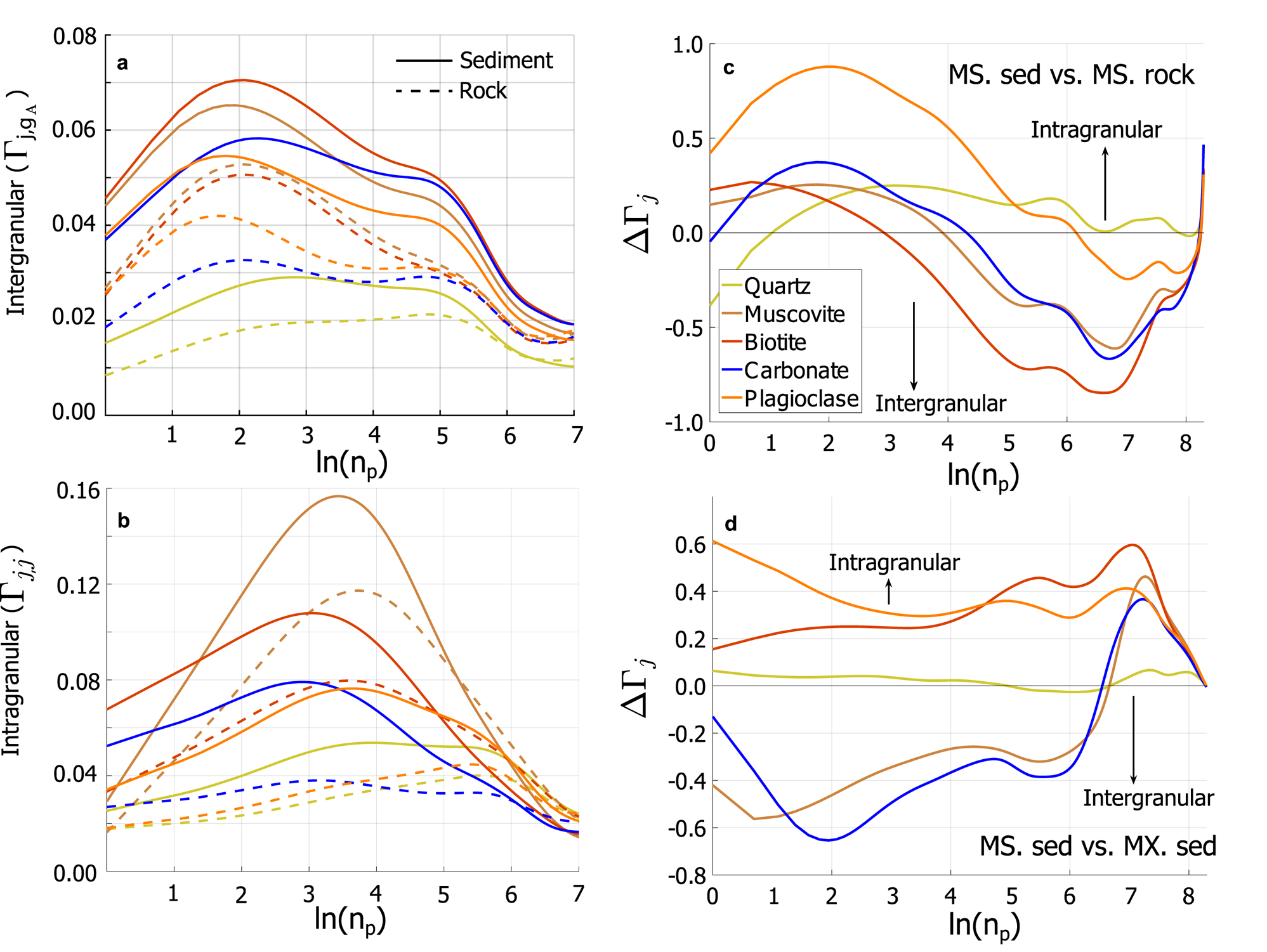
Fig. 9. Distribution of contact lengths for each mineral. (a) Normalized intergranular ($\Gamma _{j\comma g_{A}}$ ) and (b) intragranular (Γj,j) contact lengths as a function of the number of neighbouring pixel contacts (n p) for all metasedimentary sediment samples combined (solid lines) and all metasedimentary rock fragments combined (dashed lines). (c) Relative frequency of intra- and intergranular fracture (ΔΓj(D i)) between metasedimentary sediment (MS. sed) and metasedimentary rock (MS. rock) from lumped analysis. (d) Difference in the ratio of the normalized number of intragranular and intergranular contact lengths between metasedimentary sediment (MS. sed) and mixed-lithology (MX. sed). All distributions smoothed with spline estimates.
The sediment shows a lower normalized number intergranular contacts than rock fragments (Γj,g(n p)) across all sizes for carbonate–biotite, quartz–biotite, carbonate–muscovite, quartz–carbonate and muscovite-quartz pairs. This is only true above a given contact length at the boundaries of biotite–muscovite, plagioclase–muscovite and plagioclase–carbonate (n p ≈ 30) and plagioclase–quartz (n p ≈ 24), indicating that large mineral-boundary contacts are less stable than relatively short ones for these mineral pairs.
For all minerals, the number of normalized intragranular contacts (Γj,j(n p), Fig. 9b) is greater for sediment than rock fragments below a given contact length, which is n p = 1340 for quartz, n p = 735 for plagioclase, n p = 480 for carbonate, n p = 180 for muscovite and n p = 135 for biotite. Intragranular fracture is likely occurring both above and below the critical length, but with a net accumulation of intragranular contacts at short contact lengths.
Comparing intra- versus intergranular contact lengths
In comparing the relative extents of intra- versus intergranular fracture between metasedimentary rock fragments and sediment, the ΔΓj(n p) distributions show a switch in the dominant mode of failure at a given contact length. Intragranular fracture is more likely than intergranular fracture for quartz, except at the smallest grain sizes (Fig. 9c). All other minerals show that intragranular fracture dominates at small contact lengths while intergranular fracture dominates at large contact lengths. The contact length at which the dominant mode switches from intra- to intergranular fracture decreases in order from plagioclase to carbonate to muscovite to biotite.
In comparing the intra- versus intergranular contact lengths between metasedimentary and mixed-lithology sediments, we observe that plagioclase and biotite have relatively greater normalized intergranular contact lengths in metasedimentary sediments than in mixed-lithology sediments (Fig. 9d). Alternatively, muscovite and carbonate have greater intergranular contact lengths in metasedimentary sediment for all but the greatest contact lengths. Quartz shows the smallest difference in contact lengths between metasedimentary and mixed-lithology sediment.
Do fines undergo changes in grain shape and rounding in the presence of abrasion?
Aspect ratio
For both rock fragments and sediment, biotite and muscovite have an aspect ratio greater than two for all sizes, while the aspect ratio of tectosilicates and carbonates is less than two (Fig. 10a). We observe that the aspect ratio further increases from rock fragments to sediment for the phyllosilicates, while the carbonates and tectosilicates become more blocky. As an exception, the aspect ratio of the phyllosilicates is greater for rock than sediment at the largest grain sizes. For all minerals, the change in aspect ratio between rock fragments and sediment is roughly 20%. We also observe a bimodal distribution of aspect ratios for all minerals, with more pronounced bimodality in rock fragments than sediment, and for phyllosilicates than for all other minerals. The bimodal peaks in aspect ratio are separated by a local minimum that occurs at roughly the same locations as for the $f^A_j\lpar D_i\rpar$ distributions (~ 5 μm).

Fig. 10. Shape analysis. (a) Aspect ratio of metasedimentary sediment (solid lines) and metasedimentary rock fragments (dashed lines) for all samples combined. (b) Estimated change in grain area based on a difference in the perimeter of convex hull and true grain perimeter between rock and sediment from an analysis of all metasedimentary samples combined.
Roughness
For both rock fragments and sediment, the phyllosilicates have the greatest surface roughness. Across all grain sizes, rock fragments have a greater convex hull ratio than sediment, indicating that sediments are smoother than rock fragments at a given size. The difference in roughness is statistically significant between sediment and rock, and increases with grain size for all minerals. We attribute the change in roughness (ΔP j(D i)) to rounding, which increases with size from 2 to 9% (Fig. 10b). We observe the most rounding for plagioclase, while carbonate and quartz exhibit the least. All minerals show a maximum increase in rounding at the boundary between very-fine silt and fine silt. Fourier shape analysis together with Monte Carlo simulations of grain roughness corroborate these results. Fourier shape analysis indicates that changes in rounding are not interpretable below 5 μm, and that a perceived change in roughness is not primarily controlled by changes in the aspect ratio (see Supplementary Material section 1). SEM images of Glacier 1 sediments also support the inference that grains are becoming rounded (see Fig. 4).
The amount of edge material removed by abrasion (ΔA j(D i)) allows us to model the change in area distribution ($f^A_j\lpar D_i\rpar$ ) from rock fragments to sediment. For all minerals, abrasion causes a net decrease in grain size below ~ 6 μm with a surplus of new grains being added at smaller sizes (Fig. 11). Across all sizes, the material removed by abrasion (and added to the size distribution of sediment) is not sufficient to explain the difference in area distributions between rock fragments and sediment for any mineral. The occurrence of through-going fractures is likely to explain much of the difference.

Fig. 11. Area distribution $f^A_j\lpar D_i\rpar$ modelled (black lines) from the difference in roughness between rock fragments and sediment, shown with area distribution of rock fragments (solid coloured lines) and sediment (dashed lines).
Discussion
We start by discussing whether proglacial suspended sediment characteristics are representative of comminution processes within a deforming till layer. We then discuss the three specific research questions to address the overarching objectives, i.e. the relative importance of source versus process and whether the comminution of fines is more discrete or continuous.
The source of suspended sediments in the proglacial streams
Sediment mineralogy from all samples shows that fragments from both rock types are present, indicating that erosion is occurring in the upper and lower reaches of the glacier basin. Colluvium from valley walls could represent a source of fines, but we observe that the talus fields on glacier surfaces and valley walls do not contain a significant fraction of fines. In considering sediment transport, all of the proglacial streams have sufficient energy to entrain grains of the maximum size that we measure, thus we do not expect grain-size sorting to affect results (Crompton and Flowers, Reference Crompton and Flowers2016). Fluvial processes such as percussion within an R-channel and winnowing from till are possible mechanisms of sediment-size reduction. In our analysis of fines, however, we favour the hypothesis that comminution is primarily the result of till deformation. The production of fine grains within till is demonstrated by a significant sub-sand-sized fraction in seven of the samples, which contain upwards of 5% silt and clay by mass (see Supplementary Material section 3). A dearth of sub-sand-sized grains in till from the remaining ten sites can be explained by winnowing (e.g. Fischer and Hubbard, Reference Fischer and Hubbard1999), which would be a source for the suspended sediments that we sample. By averaging the suspended sediment flux across all glaciers, we estimate an effective bedrock erosion rate of ~ 1.5 mm a$\rm ^{-1}$ , which represents a significant flux of material that could otherwise be in the till (see Supplementary Material section 4). Furthermore, borehole sediments from Glacier 1 are thought to be collected from a subglacial till layer. Borehole sediments had a lower mean grain size than proglacial sediments, but grain characteristics such as homogeneity and rounding were similar between Glacier 1 borehole and proglacial suspended sediments. The lower mean grain size of the borehole sediments can likely be explained by grain-size fractionation during sampling.
The relatively softer minerals (carbonates and phyllosilicates) are more homogeneous in sediment than in rock fragments, and in the phyllosilicates, the sediment has a higher aspect ratio than in the rock fragments. An exception occurs at the largest grain sizes. We can explain this exception by invoking comminution processes within till, whereby relatively larger grains are cushioned by smaller grains, decreasing the probability of fracture (e.g. Hooke and Iverson, Reference Hooke and Iverson1995). A padding effect could cause mechanical comminution to be less effective than electrical comminution for fracturing the largest observed grains. To further support this hypothesis, we observe an increase in grain rounding with size. As larger grains become more stable in till, an increase in grain residence time will lead to more rounding.
A grain-size fractionation from winnowing could influence the mineralogy or chemical composition of the silt-size fraction (e.g. Haldorsen, Reference Haldorsen1983; Hasholt and Hagedorn, Reference Hasholt and Hagedorn2000), though Chanudet and Fillela (Reference Chanudet and Fillela2006) suggest that colloids in the proglacial stream are representative of the bedrock composition. Chemical alteration could obscure the mineral-size reduction otherwise attributed to physical erosion, but we attempt to account for this process (see Appendix A). We observe an enrichment of illite/smectite, kaolinite, laumontite, Mg clay (likely vermiculite) and Fe-chlorite in sediment relative to rock fragments. The amount of enrichment, however, is not sufficient to explain the increased area per cent of clay-sized grains in the sediment. Our discussion is therefore based on the assumption that crushing is a first-order control on the size of fines, rather than chemical processes such as dissolution or precipitation.
The grain-size distribution of fines
A geological control on microfracture spacing and grain size
Despite differences in how electrical and mechanical comminution exploit microfractures, rock fragments and sediments from both lithologies follow a log-normal distribution of sizes with a slight bimodality, and with sizes that are much smaller than the mineral size observed in thin section. From these observations, we infer that the underlying microfracture network is log-normally distributed (e.g. Hooker et al., Reference Hooker, Laubach and Marrett2018), which is consistent with the log-normal distribution of the metre-scale bedrock discontinuity spacing measured by Crompton et al. (Reference Crompton, Flowers and Stead2018). The tight microfracture spacing for both rock types might be explained by several different factors, like the proximity of the field area to the Duke River and Denali fault systems (e.g. Cobbett and others, Reference Cobbett, Israel, Mortensen, Joyce and Crowley2017), intense post-Miocene exhumation and brittle deformation (e.g. Eisbacher and Hopkins, Reference Eisbacher and Hopkins1977; Plafker and others, Reference Plafker, Hudson, Bruns and Rubin1978; Enkelmann and others, Reference Enkelmann, Piestrzeniewicz, Falkowski, Stübner and Ehlers2017) or cooling following the emplacement of the plutonic rock.
Despite similarities in the distributions, the sedimentary, metamorphic and igneous processes that give rise to the mineral composition, shape, size, extent of cementing and microfracture spacing within rocks impart clear differences on sediment and rock fragments of both lithologies (e.g. Bandini and others, Reference Bandini, Berry, Bemporad, Sebastiani and Chicot2014; Shen and others, Reference Shen, Arson, Ferrier, West and Dai2019). For example, plutonic quartz grains with fresh microfractures (e.g. Smalley, Reference Smalley1966a) are broken down to smaller sizes with a larger standard deviation than metasedimentary quartz grains, which may have had a lower microfracture density prior to metamorphism (e.g. Gomez et al., Reference Gomez, Dowdeswell and Sharp1988; Mazzullo and Ritter, Reference Mazzullo and Ritter1991; Wright, Reference Wright1995).
In addition to differences in grain size that depend on lithology, automated mineralogy results confirm that the suspended sediment grain-size distributions differ between surge-type and non-surge-type glaciers in basins of metasedimentary lithology (Crompton and Flowers, Reference Crompton and Flowers2016). We suggest that the association between glacier type and sediment size can be explained by source-rock characteristics (see Supplementary Material section 5).
The comminution of sediment is also shown to be highly dependent on mineral hardness (e.g. Chaolu, Reference Chaolu1997), as determined by the observed correlation between the Mohs-scale hardness and the peak frequency of the mineral-area distribution. The Mohs-scale hardness is not perfectly correlated with the data, however, because it encapsulates properties like the microfracture toughness and elastic modulus (e.g. Broz et al., Reference Broz, Cook and Whitney2006), some of which might depend specifically on the geological environment. Whether a grain fracture also depends on the distribution of internal stress, as governed by the configuration of minerals within a grain (Tavares and das Neves, Reference Tavares and das Neves2008), which is shown to be unique for the embedded distribution of each mineral (see Supplementary Material section 2).
The role of comminution processes in controlling the grain-size distribution
A smaller mean grain size of sediments compared to rock fragments indicates that subglacial comminution can exploit smaller microfractures than electrical pulse disaggregation. If sediment is comminuted within till, then a complex history of grain loading and unloading (e.g. Rose and Hart, Reference Rose and Hart2008; Langroudi and others, Reference Langroudi, Jefferson, Ohara-Dhand and Smalley2014) in a persistently wet environment might promote subcritical crack growth (e.g. Atkinson, Reference Atkinson1984) that is not facilitated by EPD. Alternatively, EPD and mechanical comminution might simply be exploiting different microfractures. The smaller mean grain size of sediment, however, can likely be attributed to tangential stresses within a deforming till layer (e.g. Haldorsen, Reference Haldorsen1981) that are low or non-existent during EPD. Our results agree with previous mineral processing studies that have found that abrasion leads to a smaller mean grain size from mechanical comminution relative to EPD (e.g. Andres et al., Reference Andres, Jirestig and Timoshkin1999; Giese and others, Reference Giese2010; Wang et al., Reference Wang, Shi and Manlapig2012).
When the process of abrasion acts on sediment, we observe that the grain-size distribution remains log-normal. Similarly, for larger grain sizes, the distribution can remain fractal in a transition from crushing to abrasion (e.g. Iverson et al., Reference Iverson, Hooyer and Hooke1996; Altuhafi and Baudet, Reference Altuhafi and Baudet2011). The key difference is that the fractal distribution arises from the packing structure within till, but we suggest that the log-normality of fines is controlled by the microfracture spacing. Our data show that the coarse tail can tend towards linear in log–log space (e.g. Ma and others, Reference Ma, Zhou, Regueiro, Wang and Chang2017), but linearity is not a guarantee of power-law behaviour. The Rosin–Rammler distribution is also expected to describe grain size for grains that break according to the Weibull modulus of failure strength (e.g. Weibull, Reference Weibull1951), as determined for many geological materials (e.g. Zobeck et al., Reference Zobeck, Gill and Popham1999; Paluszny and others, Reference Paluszny, Tang, Nejati and Zimmerman2016; Ma and others, Reference Ma, Zhou, Regueiro, Wang and Chang2017). In addition, the exponential end-member of the hyperbolic distribution has been found to fit proglacial stream sediment ranging from clay- to coarse-sand size (Karlsen, Reference Karlsen1991), though fluvial processes could be controlling the distribution of the coarse grains.
Continuous rather than discrete comminution
At the smallest end of the size distribution (less than ~ 3 μm), we observe a higher frequency of grains from suspended sediments than from EPD rock fragments. Grains are likely being crushed and abraded above and below this threshold, so ~ 3 μm should not be viewed as a discrete transition between crushing and abrasion. Separating the process of crushing from abrasion is not straightforward. The fines show rounding, indicating that abrasion is taking place, but the amount of material derived from rounding is not sufficient to explain the difference in grain-size distribution between rock fragments and sediment. In addition to crushing, abrasion must also be exploiting through-going fractures to explain the difference in size. A significant change in aspect ratio between rock fragments and sediment further supports the inference of through-going fractures that follow crystallographic orientation. At larger grain sizes, crushing and abrasion are thought to generate bimodal or discrete grain-size modes for larger grains (Boulton, Reference Boulton1978; Haldorsen, Reference Haldorsen1981). Our data show a slight bimodality, but the bimodality is more pronounced in rock fragments than sediments, indicating a source-rock control. In contrast to the larger grains, the continuity of process across our observed range of fine-grain sizes supports a continuous comminution model.
Composition and size of the smallest grains
From the mineral-area and size distributions of both rock fragments and sediments, and from SEM images of sediment, we infer that a significant fraction of grains are being crushed to sub-micrometre sizes. Within the clay-sized fraction, primary minerals can account for most of the area-per cent in glacially derived sediment (~ 60% in this case), indicating that clay-sized minerals do not need to be sourced from clay minerals in the rock (cf. Haldorsen, Reference Haldorsen1983; Witus and others, Reference Witus, Branecky, Anderson, Szczuciński, Schroeder, Blankenship and Jakobsson2014; Licht and Hemming, Reference Licht and Hemming2017). Langroudi and others (Reference Langroudi, Jefferson, Ohara-Dhand and Smalley2014) highlight that the density of microfractures can explain differences in the terminal grain size observed in the experiments of Haldorsen (Reference Haldorsen1981), Iverson et al. (Reference Iverson, Hooyer and Hooke1996), Jefferson and others (Reference Jefferson, Jefferson, Assallay, Rogers and Smalley1997), Kumar and others (Reference Kumar, Jefferson, OHara-Dhand and Smalley2006) and Wright (Reference Wright1995). Similarly, a sub-silt-sized terminal grain size might be expected within our field area, while a terminal size of silt (e.g. Dreimanis and Vagners, Reference Dreimanis, Vagners and Goldthwait1971; Haldorsen, Reference Haldorsen1981; Wright, Reference Wright1995) might be expected in less geologically active areas.
Inter- and intragranular fracture within fines
A continuous spectrum
Counter to expectation, a high abundance of intergranular contacts was observed for grains smaller than silt size. As comminution proceeds from crushing to abrasion, the progression of fracture from intergranular to intragranular (or vice versa) depends specifically on the mineral pair in question and on the relative spacing and length of intra- and intergranular weaknesses, and hence grain size. The hypothesis that crushing predominantly exploits intergranular boundaries (Haldorsen, Reference Haldorsen1981; Sharp and Gomez, Reference Sharp and Gomez1986) might simply be a consequence of the relatively wide spacing of intragranular weaknesses compared to the mineral size in other field areas. Alternatively, the presence of monomineralic grains might be a misleading indicating of intergranular fracture if the intragranular fracture spacing is smaller than the mineral size. Despite a switch in the mode of inter- versus intragranular fracture at a given grain size, both types of weaknesses are being exploited during crushing and abrasion, i.e. the type of fracture being exploited is continuously distributed across size.
The role of source-rock properties
We observe significant differences in the mineral composition of grains based on rock type. The largest differences occur for the carbonate minerals, whereby homogeneous grains of calcite and dolomite are much more common in metasedimentary sediments than mixed-lithology sediments. The opposite is true for biotite. The properties of quartz-bearing grains appear to vary the least between the two lithologies.
Processes to explain the dominant style of fracture
For intra- and intergranular weaknesses of comparable strength and length, a more frequent intergranular fracture at larger microfracture lengths is occurring in the presence of abrasion. One possible explanation is that mineral boundaries are more common than intragranular weaknesses at that length. As grain size is reduced, intragranular microfractures might become more frequent than grain boundaries of a comparable length, thereby causing intragranular fracture to dominate at smaller grain sizes. Alternatively, the penetration of moisture along mineral boundaries can cause stress corrosion and subcritical crack growth (Sharp and Gomez, Reference Sharp and Gomez1986). Large intergranular boundaries might be better connected than relatively smaller ones, thereby preferentially weakening the boundary of larger grains compared to intragranular weaknesses of the same size.
Changes in grain shape and rounding of fines
Continuous rounding with size
We previously established that a change in aspect ratio and through-going fractures are both consequences of crushing and abrasion processes that vary continuously with size. Furthermore, the amount of rounding due to abrasion increases from roughly 2 to 9% across our observed size range. This also contrasts with the discrete-comminution model for larger sizes (e.g. Boulton, Reference Boulton1978; Haldorsen, Reference Haldorsen1981), where abrasion selectively rounds grains that are larger than sand. A decrease in rounding with size is, however, consistent with observation for larger grains.
Processes to explain rounding
Within sediment, the extent of rounding will depend on the internal structure, and so it might not be appropriate to compare the extent of rounding for different minerals. Furthermore, the 2-D projection of grain roughness might not capture the complex interplay of grain shape and rounding in 3-D (Dowdeswell, Reference Dowdeswell1982). In considering abrasive wear, however, surface lowering has been attributed primarily to mineral hardness (e.g. Torrance, Reference Torrance1981; Sharp and Gomez, Reference Sharp and Gomez1986). Quartz and carbonates have very different hardness values, and in theory, quartz should preferentially abrade calcite while maintaining its roughness (e.g. Drewry, Reference Drewry1986; Sharp and Gomez, Reference Sharp and Gomez1986), but our data do not show this trend. Instead, we observe that quartz is more resistant to size reduction than carbonates but that the rounding is equivalent for both. An equivalent rounding between the two can be explained by a trade-off between hardness and residence time.
Conclusion
In this study we compare the mineralogy and microfracture characteristics of glacial silt and clay to rock fragments that were liberated through electrical pulse disaggregation. We find that grain and mineral cluster sizes within glacial fines are log-normally distributed with a minimum grain size that is likely below our sub-micrometer detection limit. Counter to expectation, the clay-sized fraction is predominantly composed of comminuted primary minerals. We find that the abundances of inter- and intragranular fractures are comparable, and depend on the grain size and mineral pair in question. We suggest that the relative spacing of inter- and intragranular microfractures (which differs by rock type) is a primary control on the grain-size distribution and the mineralogy of grains. The transition from crushing to abrasion is a key process for reducing grain size via rounding and through-going fractures, and partly controls the dominant mode between inter- and intragranular fracture. The form of the grain-size distribution, however, does not depend on whether crushing or abrasion dominates, as suggested for larger grain sizes. In the presence of abrasion, rounding and the relative abundance of inter- versus intragranular fracture are continuously distributed across grain size, with the extent of size reduction being dependent on the Mohs-scale hardness. In summary, the comminution of fines depends primarily on source-rock characteristics and results in a continuous distribution of characteristics across grain size. A continuous-comminution model for fines is in contrast with the larger grain sizes, where distinct grain size modes are thought to be exploited and produced in a more discrete manner.
Our findings have implications for interpreting the genesis of clay- and silt-sized material at the Earth surface and in sedimentary records used to unravel glacial history. Furthermore, debates as to whether glaciers enhance or diminish chemical weathering and the drawdown of atmospheric CO2 are highly dependent on the production rate of mineral surfaces. Our work shows that fresh primary mineral surface area peaks in the clay-size fraction, thereby strengthening the idea that glaciers are key components of the global chemical weathering cycle. If bedrock mineralogy and microfracture spacing control the production of clay in till, which has a significant impact on till deformation, we suggest that geological controls on microfracture spacing could have an indirect but important influence on glacier dynamics.
Supplementary material
To view supplementary material for this article, please visit https://doi.org/10.1017/aog.2019.45.
Acknowledgments
We thank the Kluane First Nation for granting us permission to work in their traditional territory, and Parks Canada and the Yukon Territorial Government for access permits. We are grateful for financial support provided by the Natural Sciences and Engineering Research Council of Canada (Discovery Grant, Northern Research Supplement, and postgraduate scholarships to JWC), the Association of Canadian Universities for Northern Studies, the Yukon Geological Survey, Simon Fraser University, the Northern Scientific Training Program and the Polar Continental Shelf Program. This manuscript benefited greatly from comments by the editor and two anonymous reviewers. We thank Matt Power at SGS for the QEMSCAN analysis, Shaun McDonald at SFU for a discussion of statistical techniques and Doug Stead at SFU for valuable feedback on rock mechanics.
Appendix A. Mineral selection
Chemical alterations from rock to sediment can result in a misleading interpretation of physical changes. For example, biotite appears to be weathering to illite/smectite and Mg clay (work in progress), which could lead to an apparent reduction in the size of biotite. We also need to account for mineral phases that might be inaccurately identified (e.g. Beckingham and others, Reference Beckingham2016). Edge effects from the QEMSCAN® analysis can provide a misleading interpretation of the mineralogy. For example, muscovite that borders quartz might be interpreted as illite. To limit the influence of these effects, we group various mineral phases together in the analysis, and focus on five of the most abundant minerals: quartz, plagioclase, carbonate, biotite and muscovite. Plagioclase includes all members of the solid-solution series from albite to anorthite. Carbonate includes both dolomite-ankerite (Fe or Mg rich) and calcite. Biotite also includes illite/smectite, vermiculite and Mg clay when these phases neighbour biotite, or if these phases connect through each other to terminate at biotite. Muscovite also includes adjacent illite/smectite. If illite/smectite occurs at a bridge between biotite (and its related phases) and muscovite, preference is given to assign illite/smectite as muscovite given the highly pervasive association between illite/smectite and muscovite at the boundary of muscovite grains. Illite and smectite are grouped because they are not distinguished by our analytical techniques.
Appendix B. Metrics
B.0.1. Frequency and area distributions of grains and mineral clusters
Each pixel has a length of 0.66 μm. An approximation of the 2-D grain area is A i = (0.66 μm) 2n i, where n i is the number of pixels in the i th size class, where the maximum size class is i max. We take the grain size to be the diameter of an equal-area circle: $D_i = \sqrt {{4}/{\pi } A_i}$ . The grain-size distribution is defined as

where N i is the number of grains of D i. We explore the goodness-of-fit to the size distribution with Weibull ($f=a_1a_2D^{a_2-1}e^{a_1D^{a_2}}$ ), log-normal ($f=a_1e^{\lpar {-\lpar ln\lsqb D\rsqb -a_2\rpar ^2}\rpar /{a_3}}$
 ), power law or fractal ($f=a_1D^{-a_2}$
 ) and exponential ($f=a_1e^{-a_2D}$
 ) distributions. For the Weibull, log-normal and exponential distributions, the grain-size distribution is fit to a truncated portion of the theoretical distribution using the non-linear least-squares fit function in Matlab. Parameters of the power-law distributions are estimated using a least-squares regression in ln[f ]–ln[D i] space.
In addition to analysing the size of an entire grain, we analyse the size distribution of mineral clusters within grains. The mineral-size distribution $N^c_j\lpar D_k\rpar$ is defined as the number of clusters of mineral j of a given cluster size D k across the k th of k max size classes

We explore the goodness-of-fit to cluster sizes using the same distributions listed above. Clusters of a given size can be hosted in grains of equal or larger sizes, but the distribution of $N^c_j\lpar D_k\rpar$ does not take into account the grain size. To quantify the distribution of cluster sizes as a function of the grain size, we compute what we term the ‘embedded’ distribution of the k th cluster size as

A brief summary of the results for the embedded distribution is given in the Results section. Supporting information for the methods, results and interpretation is given in Supplementary Material section 2.
The area distribution of a given mineral j is written

Equation (B4) describes the area fraction of mineral j within a grain-size class relative to the area of mineral j across all grain-size classes. The abundance of mineral j relative to all other minerals in a grain-size class is written
The shape of the distributions $f^A_j\lpar D_i\rpar$ and ψj(D i) is in dependent of the cumulative area per cent of mineral j. Note that $f^A_j\lpar D_i\rpar$
 is a probability density function but ψ(D i) is not. We also analyse the bulk area-per cent mineralogy for rock fragments and sediment.
We define an additional metric that we term the grain homogeneity, intended to characterize how monomineralic a grain is for a given mineral. Grain homogeneity differs from polycrystallinity (e.g. Gomez et al., Reference Gomez, Dowdeswell and Sharp1988); we cannot differentiate neighbouring crystals of the same mineral phase using automated mineralogy, and thus cannot assess polycrystallinity in our analysis. Thin sections of our rock samples show a high abundance of polycrystalline quartz (Fig. 2). We define the grain homogeneity for the l th grain and the j th mineral as

For l max grains in the i th size class, a mean homogeneity with respect to the j th mineral $\bar {h}_j\lpar D_i\rpar$ is computed as

B.0.2. Intra- and intergranular fracture lengths
Identifying the number of contacts n p between pixels of the same or different mineral phases (mineral pairs) allows us to estimate the extent of intra- and intergranular fracture between rock fragments and sediments. The term intragranular denotes fractures within a mineral. Intragranular microfractures can cross mineral boundaries to become transgranular, but we cannot make this distinction with our data. From automated mineralogy, we cannot differentiate neighbouring grains of the same mineral phase. To characterize the relative extents of intra- versus intergranular fractures, we start by counting the number of mineral pair contacts between a pixel and its eight neighbouring pixels for every pixel in every grain. Across all grains, we can then determine the number of contacts for each of the possible p max contact lengths. Here we use the term contact length to denote the number of neighbouring pixels for a given mineral pair. The number of within-mineral contacts for the j th mineral is

where there are N j,j,p contacts of length n p. Different grains that house contacts of the same length can be different grain sizes given the configuration of mineral clusters that make up the grain shape. To define a contact probability that depends on contact length, we define a distribution for the contact density Γj,j(n p) for within-mineral contacts of the j th mineral:

In equation (B9), the denominator term $N^e_{j\comma p}$ denotes the number of contacts of length n p of all contact types for the j th mineral, including within-mineral contacts, grain edges and mineral-boundary contacts with all other minerals.
The distribution of intergranular contacts between the j th and g th minerals is written as

Alternatively, we can compute the average contact length of a mineral j with all other minerals as

where g A denotes the sum over all minerals, but j ≠ g, i.e. we only consider contacts between mineral j and pixels of all other minerals. The difference in within-mineral (B9) versus mineral-boundary (B11) contact densities between rock fragments and sediment is interpreted as the amount of intragranular versus intergranular fracture, respectively, which is written as

In equation (B12), the superscripts s and r represent sediment and rock fragments, respectively. An example of the computation of the various Γ metrics is shown for muscovite in Figure 12.

Fig. 12. Distribution of normalized contact lengths for muscovite. (a) Normalized intragranular (circles) and intergranular (triangles) contact lengths for rock fragments (black) and sediment (red). Solid and dashed lines show spline estimates of each distribution. (b) Ratio of intragranular contact lengths of sediment versus rock (intragranular fracture, solid black line) and the ratio of intergranular contact lengths of sediment versus rock (intergranular fracture, dashed black line). The difference in ratios is the ΔΓj(D i) distribution (blue line). For a difference greater than zero, intragranular fracture dominates.
B.0.3. Shape
To analyse the shape as a function of mineralogy, we isolate grains that contain more than 90% of the mineral of interest by area. This approach might skew the results to favour the shapes of monomineralic grains, but is a straightforward approach to understanding the influence of mineralogy on shape. The shape of each grain is characterized using the aspect ratio and perimeter roughness. To determine the shape metrics, we start by computing the perimeter radius from the centre of mass as a function of the angle (Fig. 13). The aspect ratio is computed as the ratio of long to short axes, with each axis passing through the centre of mass. To find the long axis we linearly interpolate between perimeter pixels at 0.1° increments, then find the maximum distance between pairs of perimeter points 180° apart. The short axis is taken by finding the intersection between a line segment perpendicular to the long axis and a line segment linearly interpolated between perimeter points.

Fig. 13. Perimeter of the convex hull for a sediment grain from Glacier 1. (a) The true grain perimeter shown by the cross hatched blue line, with the convex hull outlined in black. Minor and major axes are shown intersecting the centre of mass. (b) Grain perimeter and perimeter of the convex hull in radius–angle space.
We measure the perimeter roughness based on the convex hull and a Fourier shape analysis. Roughness values from the Fourier shape analysis are used to estimate edge rounding based on Monte Carlo simulations of grain roughness. We use this approach to verify and supplement results from an analysis of the convex hull. Results of the Fourier shape analysis are briefly discussed herein to support the analysis of the perimeter of the convex hull, but a full discussion of methods and results is given in Supplementary Material section 1. We compute the convex hull roughness as the ratio between the perimeter of the convex hull $P^{\rm {c}}$ and true grain perimeter $P^{\rm {g}}$
 (this quantity is the square root of the Paris Factor). The convex hull is analogous to wrapping an elastic band around the edge of the 2-D grain, and therefore eliminates all concavities in the grain.
A difference in covex hull roughness between rock and sediment could result from edge abrasion. We describe the amount of material potentially removed through abrasion as the change in roughness ΔP j(D i) for the j th mineral, which is calculated as

The material removed by abrasion should lead to a decrease in grain size of the parent grain and the generation of new daughter grains. We convert ΔP j(D i) into an equivalent area of material removed as a function of the grain size in the i th size class as

Using equation (B14), we calculate a hypothetical difference in the area distribution $f^A_j\lpar D_i\rpar$ between rock fragments and sediments for each mineral. A decrease in the area distribution at size q is

where the superscripts ab and r represent the area removed by abrasion and the distribution for rock fragments, respectively. We can add the amount of material removed at size q to the area in the corresponding i th size class as

where the superscript ad refers to the material that is added to sizes with an index of i < q. We compute (B15) before computing (B16) at each decreasing index of q. This technique assumes that the material removed from a grain of size D q is a single daughter grain of size D i, and that material derived by edge abrasion can be further abraded to generate new daughter grains.
Appendix C - Sample subsets and statistical inference
To test for statistically significant differences between groups for a given metric, we use (1) paired-comparison tests, (2) tests of independent means and (3) lumped tests. In tests 1 and 2 we compare the sample statistics of a metric from each sample, whereas test 3 allows for a comparison between groups across the full distribution of grain sizes, which depends explicitly on how grain sizes are binned (discussed below).
For the paired-comparison tests of a given metric, we test the difference in sample statistics between sediment grains and rock fragments sourced from the same basin. With the exception of Glacier 1, each basin has only one sediment sample. Some basins have multiple rock samples, and for these basins, we analyse the difference between the sediment and each rock sample. Sample statistics compared in the paired-comparison test are the mean, standard deviation, skew and kurtosis. For frequency distributions, the mean size of the j th mineral computed over all grains is

For normalized area distributions $f^A_j\lpar D_i\rpar$ and ψ j(D i), the mean (first moment) is calculated as

In the case of equation (C18), an increase in $\bar {D_j}$ from rock to sediment would indicate that a given mineral concentrates its area in grains of larger size. The second to fourth moments are similarly computed. We then test that the mean difference between rock and sediment for a given sample statistic is significantly different than zero using a two-tailed t test with α = 0.05.
For the test of independent means we search for significant differences between two groups by comparing the mean of a given sample statistic between the two groups. For example, we compare the mean of the sample skew for the $N^c_j\lpar D_i\rpar$ distribution of plagioclase of each sample between metasedimentary and mixed lithology basins. For this test we use Tukey-HSD to more conservatively account for family-wise error rate, and use a significance of α = 0.05.
In addition to the test of independent means, we use principal component analysis (PCA) to qualitatively identify whether a metric can be significantly different between groups on the basis of discrete grain-size classes. To compute the principal components, we use variables composed of the terms being summed on the right-hand side of equations C17 (see Crompton and Flowers, Reference Crompton and Flowers2016 or Davis and Sampson, Reference Davis and Sampson2002) and C18.
For the lumped tests, we compare the difference in distributions between two groups across all grain sizes within a distribution. In this case, the distribution is made up of all grains from a given group, e.g. all grains from all metasedimentary sediment sample. This type of lumped analysis substantially increases the number of grains within a grain-size class, and weights the results from each glacier by the number of individual grains within a given rock or sediment sample. Some samples might therefore be over- or under-represented, though the converse is true for tests of independent means. A lumped test may not be appropriate for all circumstances, given the variation in rock characteristics within the metasedimentary lithologies across the study area. However, processes such as grain rounding might be less sensitive to source-rock characteristics and more sensitive to glacier processes. Lumping all grains or fragments allows for the detection of small yet statistically significant differences, because the number of grains increases by a factor of roughly 20 or 40 between test 3 and tests 1 and 2. A justification for using tests that combine samples across all basins (tests 2 and 3) is that the rock sample from a given basin is not always the best representation of the sediment sampled from that same basin; many of the units within the metasedimentary lithology appear to span several basins.
The size-class limits for a given range of grain sizes depend on the metric being used. For metrics that are dependent on the frequency of grains or area within a given size class (i.e. f(D i), $f^A_j\lpar D_i\rpar$ , $N_{j}^c\lpar D_k\rpar$
 , $N^d_{j\comma k}\lpar D_i\rpar$
 and ΔΓj(n p)), we use every possible discrete grain size as a separate class (i.e. i = 1, 2, 3 · · · 1250 pixels). At larger grain sizes, the distributions can exhibit significant scatter, especially when plotted in log–log space as the frequency can alternate between zero and several grains. For a clearer visual representation of a given metric, we apply a smoothing spline to the cumulative distribution function (CDF), then numerically differentiate the smoothed CDF to obtain a smoothed frequency or density function. For metrics that depend on a fractional distribution with a size class (i.e. ψ j(D i), $\bar {h}_j\lpar D_i\rpar$
 ), we find that the numerical differentiation of a smoothed CDF does not result in a representative density function. Instead, we choose a series of size-class limits such that the first 12 classes are discrete pixels sizes, and the remaining 13–20 classes are set using equal probability class sizes. The first 12 size classes each have a higher number of grains than any size class beyond 12 pixels. We determine the size-class spacing based on all sediment grains from all metasedimentary samples, but the size-class limits are applied to all groups of samples to allow for consistency across samples.


 Open access