2.1. Notation

The following notation will be used: (x, z) are the horizontal and vertical spatial coordinates; π is the excess pressure, associated with the pressure p by the relation π = p − ρ _i g(ℓ – z); ℓ(x) is the upper-surface elevation; ℓ′ = dℓ/dx, z ₀(x) is the lower-surface profile, which coincides with the bed elevation when x < 0; τ _xx , τ _zz , τ _xz are the components of the stress deviator; (u, w) is the velocity vector; η is the viscosity; f ⁺ , (−f ⁻) are the accumulation rates on the upper and the lower surfaces, respectively (f ⁻ = 0, x < 0); g is the acceleration clue to gravity; ρ _i, ρ _w are the ice and water densities; k _ρ = ρ _i ,/ρ _w; δ = 1 − ρ _i /ρ _w; δ = 1 − ρ _i/ρ _w; z ^* is the water level; [υ] is the scale magnitude of υ (for any variable υ) in the grounded pan of the glacier; (−x _d) is the position of the ice divide; x _c is the position of the ice front; σ and τ are the resultant normal and shear forces.

2.2. Setting the Problem

Considering a two-dimensional glacier merging into the ocean (Fig. 1), let us place the origin of a rectangular righthand coordinate system (z axis is directed vertically upwards) at the bed at the grounding line. Then, the regions (-x _d) < x < 0 and 0 < x < x _c, where (−x _d), x _c are the positions of the ice divide (dome) and the ice front, define the grounded and floating parts of the glacier, respectively.

Fig. 1. Schematic representation of a marine glacier consisting of different parts (grounded ice sheet, ice shelf, ice-sheet–ice-shelf transition zone) which are characterized by specific flow patterns (shearing, plug and transition). The origin of the rectangular lefthand coordinate system is set at the bed at the grounding line.

Stationary ice flow, assuming incompressibility and constant viscosity of the ice, can be described by the following Stokes’ equations:

(1)

The above set of equations must be completed by the following boundary conditions:

The glacier upper surface is stress-free and the kinematic boundary condition is used to determine its profile:

(2)

The no-slip condition at the bed may be assumed for the cold Antarctic ice sheet, where sliding is negligible (Fowler, 1981):

(3)

At the submerged lower surface of the ice shelf, the shear stress is zero, the normal stress is equal to the water pressure and a kinematic boundary condition is applied:

(4)

At the ice divide, the mass flux is zero and the fluid flow is symmetric:

(5)

At the ice front, where calving takes place, it is sufficient to impose the value of the resultant normal stress in the ice, whose magnitude in water is known (Weertman, 1957):

(6)

As we will see later, the solution of the problem does not depend on the ice-front position, whose existence is necessary only to derive the relation (6), Thus, let us assume that there is no calving and that x _c is the point of zero mass flux: q(x _c) = [inline-image] (f ⁺ − f ⁻) dx = 0, or x _c = +∞ when the mass flux is positive everywhere: q(x) > 0, ∀x > 0.

We introduce the resultant forces at an arbitrary cross-section:

Integrating Equation (1) with respect to z from z ₀ to ℓ and taking into account the boundary conditions (2), (3) and (4), we obtain the following equations:

(7)

(8)

(9)

Integrating Equation (8) with respect to x and using Equation (6), we have for x > 0:

(10)

2.3. Non-Dimensionalization

Far from the ocean, the ice flow is described by the shallow-ice approximation (Hutter, 1983), where the shear stress is much larger than the normal stress. Non-dimensionalizing the governing equations, with the following scales found by Salamatin and Mazo (1984) on the basis of similarity theory:

(11)

we obtain the following equations (capital letters denote the dimensionless variables Τ _xx = τ _xx /[τ _xx ]):

(12)

(13)

(14)

(15)

(16)

Most of the cold marine glaciers are characterized by a value of the parameter ε ≪ 1. This parameter is the typical ice-surface slope and reflects exterior conditions of the glacier’s existence, such as the scales of accumulation rate, its gradient, bed slope and water level.

In order to analyse the problem in Equations (12)–(16), we introduce the stream function ψ:

From the Equations (12) and boundary conditions (13)–(16), we obtain the following set of equations to determine ψ when L and Z ₀ are given:

(17)

Z = L (X):

(18)

(19)

(20)

(21)

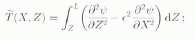
Having determined ψ, we can find all the unknown fields except the excess pressure Π as well as L and Z ₀ (X > 0). In older to find Π, we use the first equation of (12) integrated from Z to L and the boundary conditions (13) to obtain, in terms in ψ,

(22)

Let ns define

then

Because the relations (8) and (9) are derived by integration of Equations (1) with respect to z using the boundary conditions on the upper and lower surfaces, some of which were not used in the system of Equations (17)–(21), these relations can be considered as the equations to determine L and Z ₀, when X > 0. Converting Equations (8) and (9) into dimensionless form and substituting for Π via Equation (22), we obtain the following equations for L and Z ₀, when X > 0:

(23)

(24)

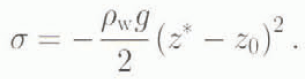
In order to determine L in the region X < 0, we integrate Equation (7) with respect to X from X to 0. Since Σ(0) = σ(0)/[σ] = −Z ^*2 /2k _ρ , this yields in dimensionless form:

(25)

3.1. Far-field Solution for the Grounded Ice Mass

We seek an expansion for ψ ^(g) , L ^(g) in the far field for the region X < 0 as an asymptotic series in ε:

Then, from Equations (17)–(21) we derive

where Q = [inline-image] F ⁺ dX. This solution describes Poiseuille flow.

From Equation (25), we have for L[inline-image] that

Differentiating this equation with respect to X, we find

(26)

It should be noted that [inline-image] only satisfies boundary conditions at the bed and the upper surface of the glacier, since all the X derivatives in the problem for [inline-image] were omitted. These boundary conditions imply that mass flux at the ice divide is zero. Equation (26) allows us to determine the upper-surface profile of the glacier far from the grounding line. However, in order to derive a unique solution to the far-field problem, it is necessary to determine the far-field surface elevation at the grounding line L ₀ ^(g) (0), as well as the magnitude of x _d, which is also unknown. These parameters are to be determined from the matching procedure.

In general, we cannot expect the stream function we have found to satisfy all the conditions at the ice divide, since the shear stress there is zero, although we have assumed that shear stresses dominate normal stresses in the shallow-ice approximation. A local expansion near the dome may be necessary but it can be shown, at least for constant viscosity, that the far-field solution is in fact valid up to the divide. Details of this derivation will be given elsewhere.

3.2. Far-Field Solution for the Ice Shelf

If X > 0, and we search for the far-field solution ψ ^(s), L ^(s), [inline-image] to the set of Equations (17)–(21), (23) and (24) in the form of an asymptotic series in ε, the leading-order term of the ice thickness proves to be zero. Hence, for the ice shelf, it is necessary to introduce its own far-field variables. In this theoretical study, where no caking is assumed and the ice shelf can be of infinite length, we suppose that far from the grounding line the scale of the longitudinal coordinate is the same as that for the grounded ice sheet. Hence, only the scale of the vertical coordinate must change. Only one transformation gives us non-zero leading-order ice thickness in the ice shelf, namely [inline-image], [inline-image], [inline-image], [inline-image]. Therefore, the coordinate [inline-image] must be taken as the far-field vertical coordinate for the ice shelf. Notice that, in terms of the grounded ice-sheet scale, the ice-shelf thickness is of order ε, which dimensionally corresponds to a scale of only a metre or so. It is to be emphasized that this scale is only appropriate thousands of kilometres from the grounding line and, in reality, calving of icebergs causes ice shelves to be much shorter (and hence thicker). Expanding the unknown functions as power series in ε:

we can find a far-field solution in the following form (for convenience, all the formulae are written in the far-field variables of the grounded part):

(27)

where

and A is constant.

The far-field solution we have found coincides with that derived by Van der Veen (1983). The constant A is to be determined from the matching procedure.

As mentioned above, we note that for X = O(1), that is, at a distance from the grounding line comparable with the grounded ice-sheet length, H = O(ε). However, the value of the constant A found by the matching procedure turns out to be such that H is O((ε/δ)[inline-image]) in the vicinity of the grounding line. Numerically, this is around 0.2, corresponding to a thickness in the vicinity of 500 m, as is observed.

If we compare the far-field solutions for the stream function in the different regions, it is clear that these are essentially different and cannot be matched. Therefore, a near-field solution in the vicinity of the grounding line is necessary to match the solution for the grounded part to that for the ice shelf. This near-field solution defines the ice-sheet–ice-shelf transition zone.

4.1. Equations

In the original coordinate system, the gradients of the fields are proportional to ε, whose value is imposed by the external conditions, such as the scales of accumulation rate, its gradient and the bed slope. But, in the ice-sheet–ice-shelf transition zone, the velocity gradient is imposed mainly by the transition from no-slip to free-floating. This allows us to make the assumption that the longitudinal scale of the transition zone is the same as the vertical one; the ratio between these does not depend on ε.

Denoting the ice thickness at the grounding line in the scales of the grounded part by L ₀, let us introduce the near-field coordinates and variables:

Rewriting Equations (17)–(21) in the new variables and neglecting bed roughness, we derive

(28)

(29)

(30)

(31)

(32)

The conditions (32) are sufficient for matching the near-field stream function with those of the far fields. Equations (28)–(32) define ψ. For the functions χ and h, it follows from Equations (23)–(25) that we have the following equations:

(33)

(34)

(35)

From Equations (23) and (24), χ,ϑ and ϑ* can be expressed via h and T:

(36)

(37)

(38)

Asymptotic analysis of Equation (34) shows that

These eases contradict the assumption of finite longitudinal scale of the transition zone.

Hence, we have, β = O(1), as ε → 0, so that β = constant + O(ε). This is a rigorous result of the asymptotic analysis of Equation (34). It is also true for non-isothermal glaciers or ice sheets with non-zero bed roughness, as the former equation does not change, except for the expressions for T and B. Then we can find the scale of the ice thickness at the grounding line Δ₀, taking β = 1 (for example) in Equation (35):

As a result, we can conclude that, assuming the average grounded ice thickness is O(1) (corresponding to 3000 m), the typical ice thicknesses for the transition zone and the ice shelf (sufficiently far from the grounding line) will be O((ε/δ)[inline-image]) (corresponding to a thickness of 800 m) and O(ε) (corresponding to 6 m), respectively, when ε = 2 × 10⁻³.

4.2. Expansion in ε

We seek the solution of Equations (28)–(38) as an asymptotic series in ε:

For the leading-order terms, we have the following set of equations:

(39)

(40)

(41)

(42)

(43)

(44)

The derived equations describe the ice flow in the transition zone. To order O(ε), the bed slope and the mass accumulation can be neglected. The parameter β ₀, as well as the values L ₀ ^(g) and A, is to be determined from matching the near and far fields.

4.3. Expansions in δ

Equations (39)–(44) also include the parameter δ, which for the process under consideration is small: δ ≈ 0.1. Therefore, the solution to the equations can be sought for as a power series of δ:

Then, for ψ _∞ and h _∞, we have the following set of equations:

(45)

(46)

Due to Equations (40)–(44), we obtain

(47)

Hence, we conclude that χ_∞ = 1; in other words, the ice upper surface is, to order O(δ), a straight horizontal line. It is notable that determination of the functions ψ, h and ϑ to order O(δ) permits the determination of χ and ϑ* to order O(δ ²).

Solving Equations (45) and (46) analytically is difficult; therefore, we use computational methods. The algorithm we use requires two initial conditions for h _∞ at the point ξ = 0. Also, the Equations (45) and (46) include the unknown parameter β _∞, whose determination needs another imposed relation. It can be shown (see the Appendix) that these conditions are

(48)

and there exists a unique solution of Equations (45) and (46).

Ultimately, the set of Equations (45)–(48) defines the unique near-field solution, including a determination of the parameter β _∞. Let us call this set the “principal system of equations”.

5. Matching Procedure

5.1. Matching the Near-Field Solution for the Transition Zone with the Far-Field One for the Glacier Grounded Part.

In order to find the unknown parameter L ₀ ^(g) for the far-field solution of the mounded glacier part, let us introduce the quantity λ = L ₀ ^(g) /L ₀ = λ₀ + δλ₁ + O(δ ²).

Matching the glacier upper-surface profiles of the far-field solution and the near-field one can be carried out by using the intermediate asymptotic variable ω = X/v(ε), where εfv → 0 and v → 0 as ε → 0 (Cole, 1968). In this way, all the unknown parameters can be found:

(49)

Then, an expression for the ice upper-surface profile [inline-image], which is valid all the way from the divide to the grounding line, can be written in the form

It should be noted that the parameter λ is determined by solving the principal system of equations and is the deviation of the far-field ice thickness at the grounding line from the near-field one there.

5.2. Matching the Near-Field Solution for the Transition Zone with the Far-Field One for the Ice Shelf

Matching the far-field ice thickness and the near-field one in the same way as before, we can find the last unknown constant A = Α ₁ δ ^2/3 ε ^4/3 β ₀ ^1/3 /4, where A ₁, is determined from the near-field solution. Then, the upper-surface profile and the ice-thickness distribution, which are valid throughout from the grounding line to the ice front, take the forms:

However, since the ice thickness in the ice-shelf region (far horn the grounding line) is proportional to ε. and the accuracy of the determination of the lower-surface profile is in O(δ), the elevation of this surface which is valid throughout and is found by the standard procedure as before, will exceed the upper-surface elevation fairly far from the grounding line. For this reason, it is convenient to find the lower-surface profile with formula (42), which is valid everywhere for the floating ice:

6. Overall Algorithm for Solving the Problem

First, it is necessary to solve the principal system of equations. As a result, the functions ψ _∞, h _∞ and the parameter β _∞ can be found. The functions χ₀, ϑ ₀ ^* and ϑ ₀ are determined to various orders of accuracy by the formulae in Equations (47).

Let its move the origin of the coordinate system to the bed at the divide, whose position is known. Then the point x = x _d defines the grounding line. Knowing β, we can find the length x _d of the grounded glacier part from the equation

(50)

which is a consequence of Equation (35). In Equation (50), the function Z ₀(x) is known, because the bed profile is given and q(x) = [inline-image].

Having determined x _d , the water depth z ^* becomes known as well as the scales of non-dimensionalization. Then, we can find the scaled ice thickness at the grounding line:

Knowledge of the value of λ₁, which is found from Equation (49), allows us to determine the glacier upper-surface profile far from the grounding line by solving Equation (26) with the initial condition: X = 0: L ₀ ^(g) = λL ₀.

The problem for the ice shell has an analytical solution. The constant A is known from the near-field solution. Then, it is easy to construct glacier-surface-profile distributions, which are valid throughout the region. Although the ice-upper-surface elevation is found to be O(δ), its gradient can be determined as O(δ ²).

It should be noted that Salamatin’s (1984) boundary condition can be transformed to the form found in this paper by choosing the proper value of the parameter which characterizes the deviation of the reduced normal deviatoric stress from its true value. Comparison of the different boundary conditions, as well as numerical methods, to solve the near-field problem will be considered elsewhere. The results of calculations are as follows:

The glacier-surface profiles are shown in Figure 2, in which we can see that the upper-surface elevation has a point of local minimum, which coincides with the conclusion of Barcilon and MacAyeal (1993). For comparison, the far-field solutions, as ξ → 0, are shown. It is clear that, at a distance of several ice thicknesses from the grounding line, the far-field solutions properly describe the ice dynamics.

Fig. 2. The near-field solutions (a) for the glacier surface profiles differ from the far-field ones (c) for − 1 < ξ < 2. There is a point of local minimum of the upper-Surface elevation. The dashed line (b) is the water level.

Several tests on the model examples were carried out to compare the grounding-line positions found using Thomas and Bentley’s (1978) boundary conditions and those derived in this paper. The difference between the results obtained is about 10% of the grounded glacier length.

7. Conclusions

The Study earned out here allows us to find strict boundary conditions at the grounding line without the use of simplifying assumptions, such as are made in the boundary-layer approximation. The parameter β is determined by the solution of the near-field problem; however, for real glaciers, it can be found by natural surveys. Changes in this parameter should reflect individual peculiarities of the specific glacier, such as sliding, temperature distributions and bed roughness.

The important result lies in the fact that the near-field ice thickness at the grounding line and that of the far field for the grounded glacier part differ from the flotation thickness by −3.3% and −0.1%, respectively. This means that the condition of hydrostatic equilibrium for the ice at the grounding line is the boundary condition for the grounded part of the glacier as well as being a proper approximation for the relationship between the ice thickness and the water depth at that line.

The glacier-surface profiles in the vicinity of the grounding line can be found separately from the solutions of the far-field problems, where the span scales are much higher. This allows us to find the glacier-surface elevation to a sufficient order of accuracy in all regions. The existence of a local minimum of the upper-surface elevation almost over the grounding line is commensurate with real glacier characteristics. This implies that the detection of such a line of local minimum elevation by surveys can point to the grounding-line position.

Our coherent approach to the study of all parts of the glaciological system (grounded ice sheet, ice shelf and transition zone) allows us to find relationships between the spatial scales of its parts via the parameters ε (typical ice-surface slope) and δ (normalized difference between ice and water densities), which characterize exterior conditions of the existence of the glacier. This also allows us to construct a complete model describing the dynamics of the system.

Despite the fad that most glaciers are essentially non-isothermal, the form of the boundary conditions at the grounding line does not change, except for the constants β and ϑ*. The case of Glen’s flow law will be considered elsewhere.