


One of the thorniest issues in social science analysis is to establish causal relationships for observational data when the options of using controlled or natural experiments are not available. We do not purport to have a solution to the general problem, but here suggest a set of novel adaptations of approaches that together can establish sequences between sets of ordinal variables, provided some key assumptions are met. “Sequences” in this paper implies a succession of realized states (regardless of the direction, duration, time, or outcome) defined as unique combinations of values across variables. One of the necessary, if not sufficient, criteria of causal relationships is that the causal factor X must exist or change before the caused factor Y. However, there are many known exceptions to this general rule, for example, the anticipation of an event such as elections that may result in a series of effects before the event itself. Given this caveat regarding interpretation, the proposed approach focuses on identifying sequences of states in manifest observational data.
Sequences are also critical to understanding many social processes such as regime transitions, onset of wars, legislative procedures, international bargaining, and institutional development. A great deal of work in political science seeks to investigate the order of occurrence of events, or utilizes historical processes to explain political outcomes. However, the sequences of complex social processes usually involve hundreds of variables with many characteristics, and today’s standard techniques for time-series cross-sectional (TSCS) analysis for observational data, are not very apt for this sort of problems. First, they do not solve the causal inference problem to a greater or lesser degree than the approach suggested here. Second, they are designed for giving insights into the average effect of x i on y given certain conditions, sometimes taking interaction effects into account. However, the social and political processes that we as social scientists are typically interested in, such as democratization, are rarely even approximations of such simplifications. Rather, complex and often long series of sequentially related variables are in play and contribute to the outcome.
We do not purport to be able to offer a complete and final solution to the disentanglement of such processes, and especially not for causally explaining the outcomes, but offer a first step toward that goal. We suggest that the approach detailed below can establish descriptive sequences in terms of necessary conditions among, in principle, an unlimited number of variables over any stretch of time, given that adequate data are available and that there are sequential relationships to be found. Thus, for example, the approach can establish that among, say, five variables x 1, … , x 5 and the outcome y, in terms of either which of the variables “moves first” and/or reaches a “high” or “full” level before others do, the sequence is x 2–x 4–x 1–x 5–x 3 and then y. Naturally, this is not equivalent to establishing that this sequence is a causal chain, or that the chain causes the outcome. However, to the extent to which one can establish that this sequence always, or almost always, precedes the outcome across time and space, we have arguably come a long way in terms of arriving at a general understanding of such a social process compared to where we are today. Until now, we have not been able to provide evidence of such sequences across time and a large number of units, other than by individual case analysis found, for example, in historical sociology and in-depth case-study approaches.
There exist several approaches for identifying sequences in ordinal and categorical time-series data, many of them more or less inspired by evolutionary biology. Noteworthy are, for example, social sequence analyses that are inspired by DNA sequence analyses (e.g., Abbott Reference Abbott1995; Abbott and Tsay Reference Abbott and Tsay2000; Gauthier et al. Reference Gauthier, Eric, Bucher and Notredame2010; Casper and Wilson Reference Casper and Wilson2015), event structure analyses (Heise Reference Heise1989; Heise Reference Heise1991), qualitative comparative analysis (QCA) (Ragin Reference Ragin1987; Rihoux and Ragin Reference Rihoux and Ragin2009), and TSCS methods (Beck Reference Beck2008). There also exists a more novel approach using Bayesian modeling to construe dynamical systems indicating flow of change (Ranganathan et al. Reference Ranganathan, Spaiser, Mann and Sumpter2014; Spaiser et al. Reference Spaiser, Ranganathan, Mann and Sumpter2014). All these methods have their pros and cons, where method choice is dependent on the format of the data and the specific question of interest.
The social sequence approach is used more frequently in political science studies. Scholars have adopted the technique to explore the careers of social movement activists (Fillieule and Blanchard Reference Fillieule and Blanchard2012), voting behavior (Buton, Lemercier and Mariot Reference Buton, Lemercier and Mariot2012), crisis bargaining patterns (Casper and Wilson Reference Casper and Wilson2015), and the evolution of regime types (Wilson Reference Wilson2014). This approach identifies the temporal order of discrete events across observations, and uses an algorithm to compare and then cluster similar sequences. It mainly focuses on describing and exploring temporal developments between different states of single variables. When analyzing multiple variables, one has to combine the categories of different variables into a single variable (Gauthier et al. Reference Gauthier, Eric, Bucher and Notredame2010). This approach is thus not suitable for data involving several variables measured on ordinal or continuous scales, as there often occurs a combinatorial explosion when combining several variables with several states into a single variable, and such an approach ignores the ordinal nature of the vast majority of variables that social scientists depend on.
We here suggest a combination of novel and pre-existing methods suitable for investigating sequences of states between two ordinal variables that change along a similar scale, with a similar step size, and with each categorical score indicating similar magnitude. These are frequency counts; transitional graphs with a graphical representation of observed changes that can be compared to expected changes; dependency analysis inspired by the logic of QCA (Ragin Reference Ragin1987; Rihoux and Ragin Reference Rihoux and Ragin2009) as well as evolutionary biology (Sillen-Tullberg Reference Sillen-Tullberg1993); and Bayesian dynamical systems (Ranganathan et al. Reference Ranganathan, Spaiser, Mann and Sumpter2014; Spaiser et al. Reference Spaiser, Ranganathan, Mann and Sumpter2014). This combination is especially useful when determining reform sequences or investigating if there are differences in paths between, for example, successful and unsuccessful attempts at democratization. By combining a number of two-variable sequence analyses, it becomes possible to describe sequences involving a large number of variables ending with a particular outcome. The approaches complement each other. The first two show how two variables differ in magnitude during transitions and the most common transition from each point. Dependency analyses more clearly show which pathways are not possible, requiring certain states to be achieved before others can be reached. While all these approaches describe raw data, finally we use all data to infer dynamical systems depicting the most expected transitional pathways from any starting point to equilibrium.
Our suggested approach differs from Granger tests for time-series data (Granger Reference Granger1969), and the standard technique of lagging variables in TSCS analyses, in one critical way. None of the approaches presented below depend on specifying a specific time interval. The one, two, sometimes five-year lags typically used in TSCS analyses are arbitrary and lack theoretical justifications. They also force the analyst to make a very strong assumption about time-invariance across units of analysis in terms of how long it takes for x to be associated with a change in y. We do not know, for example, if improvements in civil liberties such as the freedom of discussion should be expected to be associated with improvements in, say, how clean elections are, one, five, ten, or more years down the road. Furthermore, we have no theoretical reasons to assume that the time lag between changes in x and changes in y is expected to be constant across countries and over time. On the contrary, in some areas we have empirically based intuitions suggesting that we should expect time-variant time lags.
Take suffrage as an example. This was one of the main contentious issues in the 19th and early 20th century. The improvements in freedom of discussion, organization, and the right to demonstrations led to protracted processes that in many countries eventually led to full suffrage after decades. However, in the latter half of the 20th century, democratization processes starting with an opening up of the public sphere have usually (when successful) led to a rapid and immediate extension to full suffrage.
The methods proposed here do not require us to make assumptions about cross-sectional time-invariant distances in time between the occurrences or changes in the status of variables. We argue that this is one of the important advantages. As explained further below, we reshape the observational data into “states” and focus on changes between them. A “state” means the combination of a fixed value i on variable x and a fixed value j on variable y for any period of time. A change from one “state” to another is defined as a change in either i or j, or both. This structuring of the data makes it possible to map and analyze identical sequences of change, even if the length of time that country A and country B spend in various “states” varies across time. “Sequence” here means a specific series of such states, or realized conditions in a process, regardless of direction and outcome.
The first two approaches assume ordinal data, while dependency analysis can in principle be used also for continuous data. The analysis is also easier to interpret if all variables in a particular analysis have the same level of measurement, but this is not required. Finally, in order to derive differential equations, the Bayesian dynamical systems analyses require continuous data.
From the suggested frequency and dependency analyses, combining a series of such bivariate analyses (by running all variables against all), one can establish long series of sequences involving hundreds of variables. The result is a detailed and empirically based “map” of which aspects of a phenomenon occur before other aspects. In other words, we are now capable of providing the first solution to presenting detailed sequences of democratization and other similar phenomena.
The approaches here are descriptive and show what has actually happened based on the data. That is, they summarize patterns rather than test hypotheses, and the results do not say anything about the “size of effects” and cannot be used for out-of-sample predictions. Thus they do not “fail” in any formal sense, but may nevertheless show misleading patterns when applied to certain types of data (e.g., cyclical phenomena), which we will discuss further below. Nothing is claimed about causal identification either, which, as we know, is a huge issue to resolve also in standard regression formats. The approach is designed to fill a gap in an existing menu of methods, to enable us to discern sequential relationships in myriads of data points. If we have comprehensive data, then we can claim that y has always been preceded by a sequence where x 1 was realized first and followed by x 4, x 2, and x 3, in that order.
With such a set of tools at hand, we can as social scientists for the first time potentially provide empirical answers to questions like: If we want to support a democratic development in Myanmar today, where should we start? Should the efforts be directed at strengthening rule of law, or rather focus on supporting a freer media landscape, or perhaps the development of more institutionalized political parties? While causality cannot be claimed, if no country ever during the last hundred years have, let us say, managed to establish a legislature that provides efficient checks on the executive before conditions x 1 and x 2 were in place, it would seem like a reasonable recommendation that efforts be directed at conditions x 1 and x 2 before seeking to support strengthening of the legislature. These are questions to which we have until now been unable to provide much of an informed answer. The combination of the analyses below promises us to be in a much better position to answer such questions with a strong empirical foundation.
METHODS
The analysis of sequences is a tricky issue and the approach we have developed builds on combining several related approaches that in combination provide a basis for such assessments.
Frequency Tables
To explore the temporal relationship between two ordinal variables, we first look at how often pairs of values occur. We therefore construct a frequency table including all possible combinations of the values of these two variables. An example of such a frequency table for two sample variables, Variable A and Variable B, is shown in Table 1. To calculate the frequency of each combination, for each country, we first combine several yearly observations when the values of both variables do not change into one observation and count them as one “state,” regardless of how many years that combination is stable. We then count the occurrences of each combination.
Table 1 Example of a Frequency Table of Observed Combinations of Values of Two Variables
The tables show how variables co-vary in magnitude and can give us an idea of frequent and rare combinations. We may be particularly interested in whether there are clusters of values, indicating major reform paths; whether some combinations never occur; and if the common pairs of values are above or below the diagonal, or some other cut-off border. When dealing with variables of similar content, such as male versus female civil rights, we can investigate which proceeds first by comparing off-diagonal entries, but we could also use, for example, the superdiagonal (i.e., pairs of values (i, i−1)) or subdiagonal (i.e., (i, i+1)) or some other arbitrary set of values as a cut-off border, and compare values above and below the border. Unless values are roughly uniformly distributed in the table, this can give us a first indication of sequences: if values are clustered along a ridge (e.g., the diagonal), then the variables move together, and if the matrix is skewed and values are concentrated above or below the cut-off border, then one variable is largely restricted by the values of the other.
For illustration, we will here use the diagonal of the matrix as our cut-off border, assuming we are interested in directly comparing ordinal values, but the reasoning also applies to other cut-off borders. We then calculate the percentage of observations where one variable is greater than the other and compare this to the number of observations where the other variable is greater (and where they are both of the same magnitude). For example, in Table 1, Variable A is greater than Variable B in 14 cases, both are equal in 13 cases, while Variable B is never larger than Variable A. We can then do the same for Variable A and Variable C (as shown in Table 2), for example.
Table 2 Another Combination of Variables
Finally, we can (with any number of variables) construct a relative frequency table (Table 3) to systematize the number of combinations.
Table 3 Example of Relative Frequencies Table
In this case we had two heavily skewed matrices, showing that, if we compare ordinal values, C≥A≥B. We have thus found a sequence where the ordinal values of C achieve any given value x before or at the same time A does, which in turn happens before or at the same time B does.
When the variables are directly comparable, such as for the same kind of rights for different groups of people, the diagonal is a reasonable cut-off border. For other variables, there may be clear patterns of clustering or restrictions that B achieves value i only when A has achieved i−1.
However, note that other processes besides temporal sequences may lead to one variable being larger than another, for example, certain versions of periodical cycling. Thus, while the frequency analysis never “fails” in a formal sense it can nevertheless be misleading, especially when drawing conclusions where the occurrences of, say, A>C are infrequent rather than nonexistent. The supplementary methods discussed below enable visual inspection of where frequency differences originate and data structures such as cyclical variables become apparent there. We suggest no significance test for the frequency tables since they are designed for the depiction of actual sequential relationships between variables, not inferences from a sample.
Transition Graphs
Frequency analyses allow us to explore how often pairs of values occur, but they do not depict how this frequency pattern comes to be. To investigate the pathways for how variables change, we use a graphical approach as described below. Figure 1 shows the main idea behind this approach.
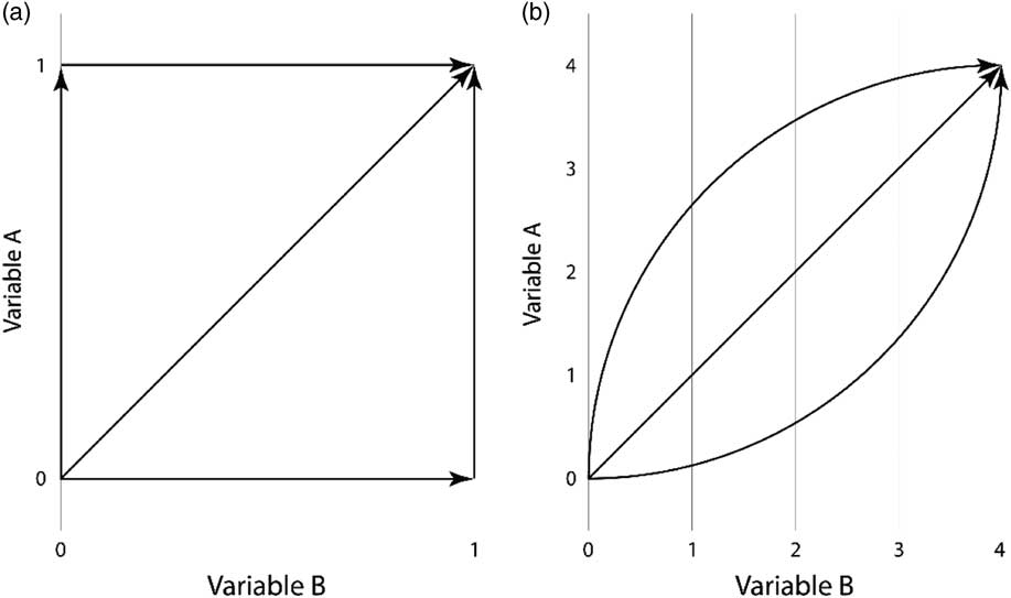
Fig. 1 Potential pathways of change in (a) two binary variables and (b) two comparable ordinal five state variables
For two binary variables, both of which take the values as 0 and 1, there are three ways for two variables to change from (0, 0) to (1, 1). Either A changes first to (1, 0); both change simultaneously to (1, 1); or B changes first to (0, 1). Thus, to determine how often A becomes 1 before B, one simply counts the number of changes from (0, 0) to (1, 1) that go via (1, 0) and compare this number to the number of changes from (0, 0) to (1, 1) that are direct, or via (0, 1) (Figure 1(a)). This counting results in a frequency table similar to Table 1, but for binary characters with only four possible combinations.
For ordinal variables the situation is more complex. Consider two comparable ordinal variables (A and B) varying along the same scale with the same step size—in our example all variables can take on the integer values 0, 1, 2, 3, and 4. The question of interest is again how one variable compares to another after a change. Partly, the general thinking is similar—if Variable A tends to be larger than Variable B, then changes ending above the diagonal will be more common than changes ending below the diagonal (Figure 1(b)), enabling the similar frequency analysis as described above.
Partly, however, the situation is entirely different, because a multitude of other potential paths are possible. For example, one variable may become larger first at lower values while the other becomes larger first at higher values; variables may go in both directions; low values of one variable may drive high values in another; or variables may be unrelated but one variable has a skewed distribution, a pattern that would result in more changes ending on one side of the diagonal even if no correlation exists between the two variables. Further, and most importantly, the variables may not be comparable—how does the value 2 for Freedom of expression truly compare to a value 2 of Alternative source information?
Looking at the frequencies of transitions between states will alleviate some of these issues. As a second type of analysis, we visually inspect the movements using a graphical approach—because of this, we term the approach graphical rather than statistical. Given a pair of values, which variable is most likely to move first? Do values revert back? This approach only illustrates one-step transitions. In order to draw conclusions about the entire transition process, the transition function of the variables is assumed to be either convex or concave, as in Figure 1(b).
To create plots indicating temporal changes in two variables, we first construct a table listing all the observed changes in values of the two variables, then produce a figure mapping all these changes (see the Results section). We report two types of figures. In the first, we map all changes using arrows indicating movement between states, where the thickness of each arrow is proportional to the number of changes that have occurred along that particular path. We also add circles in the graphs to indicate the number of times that particular combination of states is observed in the data, that is, the size of each circle is proportional to the number of observations of that particular combination. The latter are the same as the numbers reported in the frequency tables discussed above.
The other type of figure reveals reform paths that are more popular than expected by utilizing observed data (indicated by the circles in the first type of figures) to calculate a table of expected values using χ 2 methodology from the distribution of each variable. Graphing the difference between the table of observed and the table of expected values reveals reform paths that are more popular than would be expected by the distribution of the two variables alone (see the Results section).
These figures depict transition steps and identify transition chains. Assuming that variables change along a similar scale, with a similar step size, with each categorical score indicating a similar magnitude, and that no parts of the full transition processes are systematically underestimated (data are a snapshot of history, so inadvertently only a subsection of the full transition sequences may be captured), a convex function would indicate that the variable on the x-axis moves first, and a concave function that the variable on the y-axis moves first.
It may be tempting to use observed and expected tables discussed in the previous paragraph to also calculate the χ 2 statistic, but since the two tables may differ for reasons other than the existence of popular reform paths, a significance value is not necessarily meaningful—hence the emphasis here on visual inspection. If significance tests are deemed desirable (we urge caution since this requires that many assumptions are fulfilled), we instead recommend quasi-symmetric model tests for comparing off-diagonal values in square tables (Agresti Reference Agresti2013) utilized on the observed frequencies.
The transition graphs are descriptive and limited to bivariate relationships only, but can be stringed together as described above to reveal sequential relationships between several variables. The graphs can reveal very common pathways, if such exist, and, importantly, indicate pathways that have not been realized due to a lack of connecting arrows between two points. We can thus find “typical paths of change” and disprove hypotheses about paths that are not present empirically. In the next section, we look directly at how, for variables to reach given values, they are dependent on other variables reaching certain values first.
Dependency Tables
To explore whether certain values of one variable are systematically conditional on certain values of other variables in the existing data, we suggest an approach here termed dependency tables. The approach is inspired primarily by “the contingent states test,” which is an established method developed to investigate dependencies in biological evolution (Sillen-Tullberg Reference Sillen-Tullberg1993), and is particularly well suited to use on sequence data outside biology. It also has some similarities with QCA (Ragin Reference Ragin1987; Rihoux and Ragin Reference Rihoux and Ragin2009). Note that even though A and B may co-vary, the dependency tables check for absolute dependencies in the data, not statistical correlations. This is an important distinction since if one can establish such absolute dependencies—and assuming that the data are more or less complete in coverage—then this is evidence of revealing necessary conditions displayed by the data that are not contingent on analytical inferences from regression statistics and out-of-sample predictions.
To construct dependency tables, for each value of one variable, we scan the data set for the lowest value in all other variables. If a particular value in A (say “1” on a scale from 0 to 4) always correspond to a higher “lowest observed value” in B (say “3” on a scale from 0 to 4), it can be inferred that a transition from value 0 to 1 on A is conditional on value 3 on B. If simultaneously, for each value of B, the corresponding “lowest value” in A is its minimum (0), then B is not restricted by A. These two observations in combination indicate that dependencies between the two variables exist only in one direction. Dependency should not be taken as evidence of a causal relation, but only that certain values for one variable are conditional on certain values for the other in the available observations.Footnote 1
Table 4 shows an example of such a procedure. Table 4(a) indicates that higher states (2 and 3) in A occur only together with higher values in B (2 and 3, respectively). This means, for example, that A is never observed to reach value 1 before B has reached value 2. Thus, B has always reached value 2 before A “started moving.” At least, this is how it has always been so far according to the data. Table 4(b) indicates no such dependency, since A can be 0 at any level of B. Thus, A is dependent on changes of variable B having taken place at several stages, while in the opposite direction, there is no such dependency. In this case, we could conclude that improvements in B are likely to be a necessary condition for improvements in A (again without implying that there is a direct causal relationship). We can make a firmer statement regarding the opposite direction. There are no dependencies in the other direction, so improvements in B are not necessary conditions for improvements in A.
Table 4 Example of Dependency Tables
As before, by extending this to multiple pairwise comparisons, we can identify sequences involving many variables over long periods. Dependency tables can be constructed for all possible combinations of variables. There are various possible summation measures for such a series of dependency tables, each providing different sets of information useful for depicting varying stages in a transition process to focus on. We present three of these measures, depending on whether the interest is on early, late, or continuous dependencies in the transition process.
One measure is to sum all the lowest values of B indicated in the second column in Table 4 (a), giving a sum of 13. High values on this summary indicator suggest that for A to improve and reach higher states, high(er) values on B are required early on in the transition process.
Another measure is to sum the number of increments in B. There are three thresholds where B needs to increase for A to increase: B needs to be at least 2 for A to grow beyond 0; B needs to be at least 3 for A to grow beyond 1; and B needs to be 4 for A go above 2. This measure then indicates when there is a strong correlation and gradual dependence of A on B throughout the transition process.
A third measure is to look at the lowest value in Variable B when A attains its maximum value, here 4. In this example, thus, A has never reached its highest state without B being at its highest value (also 4). The reverse is not true: there are instances when B has reached its highest value 4 while A stands still at 0. Thus one can conclude that the full development of B has always preceded or come in tandem with A.
Conducting the same analysis across many variables, we can get a depiction of which variables have developed first, and which are dependent on high levels of many others and thus have come last in a sequence. A low number of dependencies for all states of B would indicate that there are very few conditions required for it to assume higher (in our case illustration below, more democratic) states. If A has many contingencies, then this indicates that it never reaches higher (more democratic) states before several other variables have reached high levels. This number is informative of the completion of a process, and of interest when investigating what is required for full implementation of an institution, reaching a state such as democracy, or a similar outcome.
Thus, we can get a good sense of which variables come first, middle, and last in processes of democratization. An example of how several such bivariate dependency tables can be summarized, is found in Table 5. In this illustration, we use the third measure: looking at the threshold value for each of the other variables for a focal variable to attain its highest value. Successively shifting focal variable, we can then summarize these threshold values and report them as “#Requisite conditions.”
Table 5 Example of Combining Dependency by Reporting, for Each Variable, the Number of Conditions (Sum of the Lowest Values for all Other Variables) Required to Reach the Highest State
In this illustration, the maximum sum of requisite conditions for a variable reaching its highest state, is 20 (five other variables, and each variable’s maximum level is four). The results would indicate that B comes first in attaining its maximum value in this sequence. It can reach its highest state completely unconditional on any other variables. E, D, and C constitute a middle group with some conditions required for them to reach their highest states. The low number of dependencies indicates that the variables upon which their highest states are conditional, are likely to be few and at relatively low states, although it could also mean a high state on one variable. (In order to know which variables these are, one would look at the summary table for each of these three variables.) Finally, F and A are the “late-comers” that have only been observed at their highest states after a greater number of other variables reaching their highest, or close to highest, states.Footnote 2 Together, this indicates a rough sequence that can be instructive for analyses of direct policy relevance.
This example of looking at the highest states dependencies, is of particular interest when one is analyzing, for example, what these conditional relationships look like for achieving democratization, understood as a country becoming fully democratic. Then it is natural to focus on the highest states of variables. If one were, for example, interested rather in the onset of transitions, then one should look at the number of dependencies for variables reaching the first, or perhaps the second, level on the ordinal scales, which would indicate “early moves” rather than “final push.” Misleading results can be the product of analyses where there are very few observations in total.
Bayesian Nonlinear Dynamical Systems
To study nonlinear dynamics in the interaction between variables, we also suggest employing a newly developed Bayesian dynamical systems analysis that models the probable reform direction of countries depending on empirical state combinations. This method identifies the best nonlinear functions that capture the interactions between two or more variables. Bayes factors are employed to decide how many interaction terms should be included in the model, with a penalty for overly complex models. The method gives a set of differential equations, one for each variable, modeling how the values in each of the variables involved affect the direction of each. From this, we can infer the most likely trajectory that a country will follow, given any starting point, and we can identify more complete expected transition trajectories, not only one-step changes, and more intricate trajectories, such as S-shaped curves, circular patterns, and feedbacks where variables are mutually dependent.
The resulting dynamical system can be illustrated by a phase portrait, where the modeled trajectories are depicted with arrows. Contrasting to the transition graphs, however, these are generalized figures, showing expected change, and will, for example, not include information on impossible paths, nor probabilities for making alternative one-step transitions to the most expected one. The raw transition graphs and dynamical systems modeled phase portraits should thus be used as complementary graphical illustrations. The method is described in detail in two papers by Spaiser et al. (Reference Spaiser, Ranganathan, Mann and Sumpter2014) and Ranganathan et al. (Reference Ranganathan, Spaiser, Mann and Sumpter2014).
Since differential equations deal with continuous variables, we use continuous versions of the V-Dem variables. It is important to note that the method provides a system for the entire set of possible values for the two variables. That is, it uses all the data points and provides a general description for the entire system, including predictions also for combinations of the two variables that do not occur in the data. For illustrative purposes, we do not plot the arrows for these points in the phase portraits.
ILLUSTRATIVE APPLICATION: THE DEVELOPMENT OF DIFFERENCE ASPECTS OF DEMOCRATIZATION
Scholars have pointed out various defining features of democracy, such as the protection of civil rights, accountability to citizens’ preferences, regular and competitive elections for the chief executive and national legislature, freedom of expression and association, and constraints on executive’s behavior (e.g., Dahl Reference Dahl1971; Dahl Reference Dahl1989; Sartori Reference Sartori1987; Diamond, Linz and Lipset Reference Diamond, Linz and Lipset1989; Schmitter and Karl Reference Schmitter and Karl1991; Schumpeter Reference Schumpeter1947; cf. Munck Reference Munck2001). In the post-Cold War era, we have seen regimes with different mixes of the democratic and authoritarian features. For example, in some countries, citizens enjoy liberal rights to a certain extent, but fail to establish competitive elections, while in others, elections take place regularly, but media is largely controlled by the incumbent party. Do some of the democratic features constitute the preconditions of other aspects and have to develop first for a successful democratic transition? What are those features? Is the improvement of some aspects more likely to lead to the enhancement of others? The approaches for identifying sequences discussed above are well suited to the task of examining the temporal relationships between different aspects of democracy in the process of regime transition. In what follows, we use the example of different components of “polyarchy” to demonstrate how the proposed approach can be utilized for such a task.
Based on Dahl’s (Reference Dahl1971) conceptualization, polyarchy refers to a political system in which rulers are responsive to the preferences of its citizens. To achieve this, the minimum requirements for polyarchy include: (1) freedom to form and join organizations, (2) freedom of expression, (3) the right to vote, (4) eligibility for public office, (5) the right to compete for support, (6) alternative sources of information, (7) free and fair elections, and (8) institutions for making government policies depend on votes and other expressions of preference. Among these requirements, items 1, 3, 4, 5, 7, and 8 focus on the mechanism of competitive elections in which all citizens should have equal opportunities to participate. These features construct citizens’ ability to make a choice that reflects their preferences in an explicit political decision-making process. The other two items, freedom of expression and alternative sources of information, concern citizens’ ability to formulate and express their political opinions. That is, these requirements enable citizens to define their goals in the public sphere.
We expect that in the process of regime change, the Freedom of expression and access to Alternative sources of information should develop before the establishment of competitive elections. In the literature on democratization, scholars have pointed out that the challenge to authoritarianism results from a preference for changing the redistributional equilibrium through democratization (Acemoglu and Robinson Reference Acemoglu and Robinson2001; Boix Reference Boix2003). For preferences about the redistribution issue to be formulated, and for the idea of a democratic system as an alternative solution to be recognized and accepted by more people, citizens must enjoy at least a certain level of freedom to discuss their government and have access to viewpoints alternative to government propaganda. That is, as different aspects of democratic governance, we expect that the improvement of citizens’ expressive freedom precede the establishment of a substantially free and fair electoral regime.
Data
To explore the temporal relationship between various aspects of democracy utilizing the proposed sequence analysis approach, we use the V-Dem dataset v4 for the purposes of presenting. V-Dem aims to achieve transparency, precision, and realistic estimates of uncertainty with respect to each data point. The v4 dataset includes 173 sovereign or semi-sovereign states with annual observations on all variables from 1900 to 2012, and covering 2013–2014 for 60 countries.Footnote 3 For each, there are observations on some 350 unique variables, and over 40 various indices related to democracy. For details on the V-Dem methodology and data set, see Pemstein, Tzelgov, Wang (Reference Pemstein, Tzelgov and Wang2015) and Coppedge et al. (Reference Coppedge, Gerring, Lindberg, Pemstein, Skaaning, Teorell, Tzelgov, Marquardt, Wang, Pernes, Stepanova, Miri, Mechkova and Andersson2015a, Reference Coppedge, Gerring, Lindberg, Teorell, Altman, Bernhard, Fish, Glynn, Hicken, Knutsen, McMann, Pemstein, Skaaning, Staton, Tzelgov, Wang, Zimmerman, Marquardt and Miri2015b, Reference Coppedge, Gerring, Lindberg, Teorell, Altman, Bernhard, Fish, Glynn, Hicken, Knutsen, McMann, Pemstein, Skaaning, Staton, Mechkova and Andersson2015c, Reference Coppedge, Gerring, Lindberg, Skaaning and Teorell2015d).
All V-Dem aggregated indices are interval variables scaled from 0 to 1. We use the ordinal versions of these—except for the dynamical systems, where we use continuous versions—as developed by Lindberg (Reference Lindberg2016). For the purpose of illustration below, we have chosen the versions of the indices with five levels.
Measures
To measure citizens’ freedom to discuss political issues and formulate opinions, we rely on V-Dem’s “Freedom of expression index” (v2x_freexp_thick), which combines the freedom of discussion and academic expression, no print, broadcast, and internet censorship, no media self-censorship, and no harassment of journalists. Another democratic feature that we are interested in is whether citizens have access to Alternative sources of information. We rely on the V-Dem “Alternative source information index” (v2xme_altinf), which measures the extent to which there is a media bias against the opposition, whether media criticize the government, and whether media represent a wide range of political perspectives. The construction of the ordinal version of these two indices is based on the procedure described above.
To capture the quality of competitive elections, we rely on the “V-Dem Electoral component index” (v2x_EDcomp_thick). Consistent with the features of polyarchy that focus on the electoral mechanism, this index combines the following elements: whether suffrage is extensive; political and civil society organizations can operate freely; elections are clean and not marred by fraud; and the chief executive is selected through elections. See the Online Appendix for descriptive statistics on these three variables. Based on the categorical version of the V-Dem indices, we can proceed with the following analyses that together constitute the new approach to sequence analysis that this paper introduces.
Illustrative Results
Spearman’s rank correlations revealed variables to be positively correlated with each other. What we aim to investigate is how movement happens between high and low values in polyarchy—are there sequences of change between the different component variables? Specifically, does the improvement of citizens’ expressive freedom and information sources precede the establishment of substantially competitive elections?
Frequency tables
The frequency tables for Freedom of expression, Alternative source information, and Electoral component index are presented in Table 6. The Electoral component index is dependent on both the other variables to attain large values, and most states are either on the diagonal or above. This suggests a transitional sequence where the ordinal value of the Electoral component index is rarely larger than the other variables, and almost exclusively never more than one unit above, meaning that Freedom of expression and Alternative source information mostly attain value i before the Electoral component index does, and almost without exception attain i−1 before the index attains i.
Table 6 Frequency Tables of the End Results of Changes in Combinations of the Traits Freedom of Expression, Alternative Source Information and Electoral Component Index

The states for pairs of values of Freedom of expression and Alternative source information are clustered along the diagonal and the super- and subdiagonal. Assuming that transitional changes happen mostly in small steps (as will be verified in the transition graphs), the two variables change mostly together or take turns in changing.
Transition graphs
In Figure 2, the left panels indicate empirical observations of all occurrences and changes in the data, while the right panels depict the difference between observed occurrences and the expected number of occurrences given the distribution of the variables. In the left-hand panels, the size of each arrow and circle is proportional to the number of observations. In the right-hand panels, the legend indicates the difference between observed and expected frequencies, indicating a “typical reform path” as designated by the yellow and gray paths. The path is “typical” because observations here are more common than they would be as expected from the distribution of the observations alone.
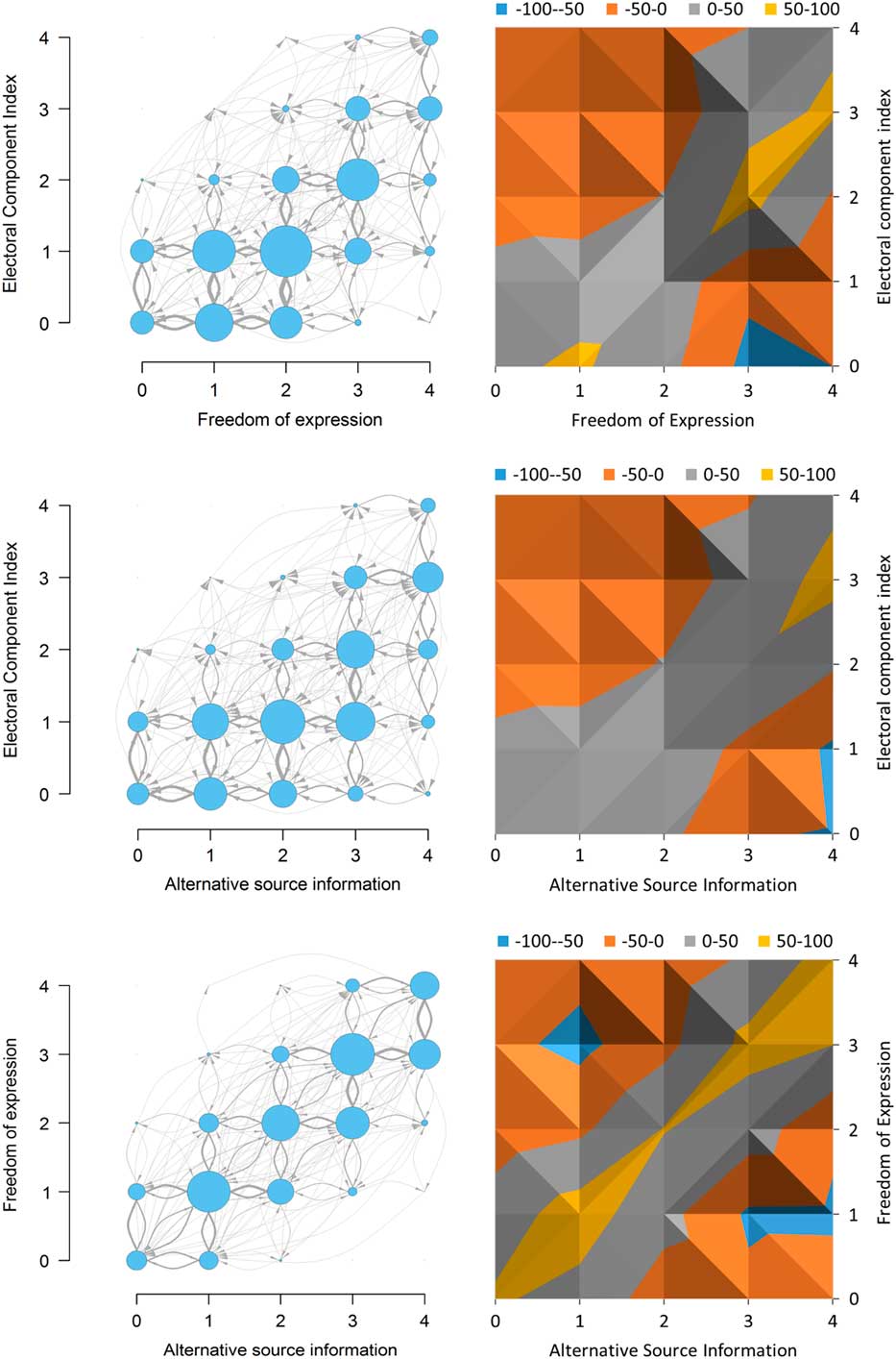
Fig. 2 Graphs showing (left) the frequencies of occurrences and changes and (right) the observed Note: Expected frequencies in the Electoral component index, Freedom of expression, and Alternative source information. The right figures indicate a “typical reform path.”
As the left panel of the figure shows, in the transitions, the two variables Freedom of expression and Alternative source information generally take on a given value i before the Electoral component index. Looking at the “typical reform path,” transitions tend to pass through states where the ordinal value of the two other variables are one step larger than the Electoral component index. Meanwhile, the start of the process may be different: there are about as many states where the electoral index is 0 and the other two variables increase from 0 to 1, as where they revert from 1 to 0. This suggests that the electoral index may first have to increase from 0 before the transition process can take off. Our fourth approach, dynamical systems, will delve further into this type of nonlinearities.
The graph for Freedom of expression and Alternative source information (the lower panel) largely confirms our assumptions and observations from the frequency tables: transitions mostly take place in small steps, and the variables change together or mostly in turn.
Dependency tables
To investigate if scoring high on the Electoral component index depends on the development of both Freedom of expression and Alternative source information, as suggested by the earlier results, we construct dependency tables. Table 6(a) documents, across all observed combinations, countries’ minimal scores for Freedom of expression and Alternative source information when the country scores 0, 1, 2, 3, or 4 on the Electoral component index. Numbers within parentheses are the absolute minimal values, while numbers outside parentheses are the fifth percentiles, which allow 5 percent margins of error. For example, there is no country scoring 3 on the Electoral component index when its level of Freedom of expression and Alternative source information is not at least 1, or 2, allowing for a 5 percent wiggle room.
To rule out the possibility that the development of Freedom of expression and Alternative source information may depend on the Electoral component index, that is, that the minimal values presented in Table 7(a) are due to correlations and not temporal dependencies, Tables 7(b) and 7(c) show the reversed descriptives to those in Table (7a). The numbers in Table (7b) and (7c) are countries’ minimal scores on the Electoral component index when the country scores 0, 1, 2, 3, or 4 for Freedom of expression and Alternative source information. The tables show that only for the highest score of Freedom of expression does the Electoral component index need to score at least 1. Note also that there are interdependencies between Freedom of expression and Alternative source information, indicating that the relationship between these two variables is more akin to a strong correlation.
Table 7 The Electoral Component Index is Dependent on Freedom of Expression and Alternative Source Information, but not the Other Way Around
Note: Freedom of expression and Alternative source information are interdependent
For analyses of sequential relationships between a larger number of variables, dependency tables can be constructed for all possible combinations of variables, and be systematized in various ways. In Appendix 2, we exemplify the resulting type of aggregate summary of some 2,000 individual analyses following the dependency tables approach, over 22 variables.
Bayesian dynamical systems
The best fit from our Bayesian dynamical systems modeling for the variables Freedom of expression (x), Alternative source information (y), and Electoral component index (z) is:
 $$\eqalignno{ & dx\,{\equals}\,\left( {{\minus}0.069x{\plus}0.024{\rm }{y \over x}{\plus}0.015{x \over y}{\plus}0.032z^{2} } \right)z \cr & dy\,{\equals}\,\left( {0.06{\minus}0.12y{\plus}0.055xy} \right)z \cr & dz\,{\equals}\,\left( {0.099{\minus}0.44z{\plus}0.31z^{2} } \right)z{\plus}0.05xy $$
The equations quantify the direction and rate of change for the variables x, y, and z, respectively, depending on current values of x, y, and z. There is an interaction between all the variables, since all of them occur in all equations. Figure 3 shows the corresponding phase portrait when including only Freedom of expression and the Electoral component index.
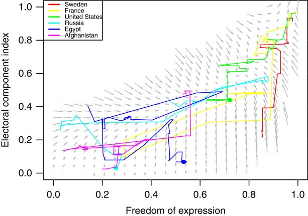
Fig. 3 Phase portrait showing the expected direction of change given different values of Freedom of expression and Electoral component index Note: Longer arrows indicate more rapid change. The figure also includes the actual trajectories of six arbitrarily chosen countries.
The dynamical system largely verifies and quantifies our previous hints from the transition graphs, but it also identifies some nonlinearities: for most of the transitions process, the Electoral component index is dependent on the other two variables before it can grow, and more so than in the other direction, except at the onset of the transition process (potentially up to one third), where the Electoral component index grows first. The first two equations do suggest that Freedom of expression and Alternative source information have an intertwined transition process, where alternative source information cannot remain at high values when there is little freedom of expression, but also that some electoral rights must be implemented before the variables can reach their highest values.
For all results, further explanations and the full analysis, see Appendix 2.
CONCLUDING DISCUSSION
This paper details a new approach to the study of sequences in social science that includes four supplementary analyses inspired primarily by evolutionary biology and Bayesian statistics: frequency tables, transition graphs, dependency tables, and Bayesian dynamical systems. The usefulness of these analytic tools and their supplementary nature is illustrated with a simple sequence analysis of three components of the V-Dem electoral democracy index and an expanded analysis to illustrate the stringing together of several pairwise comparisons for the dependency tables. We used frequency tables to get a general overview of the domain of states, finding realized and nonrealized combinations of values for variables, clusters of obvious major reform paths, and cut-off borders limiting the development of one variable before the other. This was complemented with transition graphs illustrating actual one-step movements between states, and, in the simple case, suggesting transitional sequences. We also drew inferences by modeling dynamical systems based on the data. Finally, we found dependencies between variables, where a certain value of one variable has to come before a given value of another, and used this information to initiate a multivariate sequence analysis. Our approach consists mainly of descriptive analyses that are complementary. Being descriptive, there are no strict assumptions for using the approaches, but conclusions need to be based on a combination of observations and sound reasoning.
We believe the approach has great potential for the analysis of many types of pressing issues that social science confronts, not least for sequences of democratization. We hope to use the set of tools in the near future to be able to answer critical questions of successful and unsuccessful sequences, as well as what democracy support should focus on at various stages of democratization in ways that can directly inform policy and practitioners’ priorities.


 Open access