


1 Introduction
The momentum flux or wind stress is a fundamental parameter in the study of air–sea interactions. In particular, air–sea momentum fluxes provide crucial boundary conditions for ocean, atmosphere and surface wave models. The accurate predictions of momentum exchanges between the air and the ocean require a comprehensive understanding of the turbulent boundary layer above ocean surface waves. In the past few decades, several research efforts have attempted to investigate the modification of momentum flux by surface waves (e.g. Smedman, Tjernström & Högström Reference Smedman, Tjernström and Högström1994; Donelan, Drennan & Katsaros Reference Donelan, Drennan and Katsaros1997; Drennan, Kahma & Donelan Reference Drennan, Kahma and Donelan1999; Smedman et al. Reference Smedman, Högström, Bergström, Rutgersson, Kahma and Pettersson1999, Reference Smedman, Högström, Sahlée, Drennan, Kahma, Pettersson and Zhang2009; Sullivan, McWilliams & Moeng Reference Sullivan, McWilliams and Moeng2000; Grachev & Fairall Reference Grachev and Fairall2001; Shen et al. Reference Shen, Zhang, Yue and Triantafyllou2003; Donelan et al. Reference Donelan, Babanin, Young, Banner and McCormick2005, Reference Donelan, Babanin, Young and Banner2006; Babanin et al. Reference Babanin, Banner, Young and Donelan2007; Kihara et al. Reference Kihara, Hanazaki, Mizuya and Ueda2007; Yang & Shen Reference Yang and Shen2009, Reference Yang and Shen2010; Grare, Lenain & Melville Reference Grare, Lenain and Melville2013a). For growing waves, the momentum flux is mainly downward from the atmosphere to the ocean (Smedman et al. Reference Smedman, Högström, Bergström, Rutgersson, Kahma and Pettersson1999; Grare et al. Reference Grare, Lenain and Melville2013a), while for mature seas, the momentum flux is upward from the ocean to the atmosphere (Drennan et al. Reference Drennan, Kahma and Donelan1999; Smedman et al. Reference Smedman, Högström, Bergström, Rutgersson, Kahma and Pettersson1999, Reference Smedman, Högström, Sahlée, Drennan, Kahma, Pettersson and Zhang2009). Grachev & Fairall (Reference Grachev and Fairall2001) further explained that the upward momentum flux occurs because fast-moving swells are travelling faster than the local wind when the wind and swell are in the same direction. The field measurements of Donelan et al. (Reference Donelan, Drennan and Katsaros1997) also demonstrated that the presence of swells can result in an increased drag coefficient compared to pure wind seas. However, the current understanding of momentum flux modulation by surface waves is still inadequate. Consequently, modern parameterizations of the air–sea momentum flux at the ocean surface remain insufficient, especially in strongly forced conditions (Hara & Sullivan Reference Hara and Sullivan2015). For turbulent flow over a flat rigid surface, the total stress is comprised of the viscous and turbulent stresses. The situation over wavy liquid surfaces, however, is further complicated by the fact that a component of the stress is carried by the surface waves, which may strongly impact the air–sea momentum flux. Therefore, the air–sea momentum flux or total stress over the ocean is expressed as the sum of turbulent, wave-induced and viscous stress components (e.g. Grachev et al. Reference Grachev, Fairall, Hare, Edson and Miller2003; Veron, Saxena & Misra Reference Veron, Saxena and Misra2007). Laboratory and numerical studies have allowed for systematic inquiries into these separate components of the total stress. In this paper, we examine turbulent, wave-induced and viscous stresses sequentially before evaluating the total air–water stress balance in the final section.
The turbulent Reynolds stress in an airflow is of great significance to many processes, including turbulence transport and production. The turbulent Reynolds stress was found to form a negative–positive pattern along a wave crest (e.g. Shen et al. Reference Shen, Zhang, Yue and Triantafyllou2003; Yang & Shen Reference Yang and Shen2009, Reference Yang and Shen2010; Buckley & Veron Reference Buckley and Veron2016, Reference Buckley and Veron2019). It is negative (positive) along the windward (leeward) side of the waves, which appears to be correlated with the asymmetry in the flow acceleration over the waves (Belcher & Hunt Reference Belcher and Hunt1993). Such along-wave variations of the turbulent stress were also qualitatively observed in the early laboratory studies of Hsu, Hsu & Street (Reference Hsu, Hsu and Street1981) over mechanically generated water waves. Yang & Shen (Reference Yang and Shen2009) later attributed the negative region of the Reynolds stress above the windward face to vertically bent quasi-streamwise vortices. Hudson, Dykhno & Hanratty (Reference Hudson, Dykhno and Hanratty1996), however, interpreted the regions of negative turbulent stress to be an artefact of the (fixed, Cartesian) coordinate system and argued that the turbulent stress remained positive everywhere when calculated in a boundary-layer coordinate system. In the current study, it has also been noted that the distribution of turbulent stresses over surface wind waves is sensitive to the frame of reference in which they are estimated. Furthermore, the distribution of the turbulent stress is strongly dependent on the wave age. As the wave age increases, the asymmetric distribution of the Reynolds stress along the wave crest with a positive peak region roughly above the wave trough shifts to a more symmetric distribution with a positive peak on the leeward side of the wave that extends to the upwind face of the waves (Shen et al. Reference Shen, Zhang, Yue and Triantafyllou2003; Yang & Shen Reference Yang and Shen2010). Buckley & Veron (Reference Buckley and Veron2016) related this effect to the boundary layer thickening over the wave crests. Over a wavy surface, vertical mean profiles of the turbulent Reynolds stress have a structure similar to that observed by others over flat surfaces (e.g. Grass Reference Grass1971; Aydin & Leutheusser Reference Aydin and Leutheusser1991). That is, the Reynolds stress increases with height within the inner region and then becomes almost uniform farther from the surface (Hsu et al. Reference Hsu, Hsu and Street1981; Hsu & Hsu Reference Hsu and Hsu1983; Mastenbroek et al. Reference Mastenbroek, Makin, Garat and Giovanangeli1996; Sullivan et al. Reference Sullivan, McWilliams and Moeng2000; Shaikh & Siddiqui Reference Shaikh and Siddiqui2008, Reference Shaikh and Siddiqui2010; Yang & Shen Reference Yang and Shen2010; Hara & Sullivan Reference Hara and Sullivan2015; Husain et al. Reference Husain, Hara, Buckley, Yousefi, Veron and Sullivan2019).
The wave-induced stress is important not only in transferring momentum from the wind to the waves in the wave-generation process but also in transferring energy between the mean flow and the wave-coherent motions. The early studies measuring the wave-induced stress over water waves in a laboratory, first performed by Karaki & Hsu (Reference Karaki and Hsu1968) and Stewart (Reference Stewart1970) and furthered by Hsu et al. (Reference Hsu, Hsu and Street1981) and Hsu & Hsu (Reference Hsu and Hsu1983), revealed that most of the wave-induced stress is produced near the interface, in the boundary layer where the motion is rotational. In general, the wave-induced stress is a strong function of wave conditions such as wave age (e.g. Hristov, Friehe & Miller Reference Hristov, Friehe and Miller1998; Hristov, Miller & Friehe Reference Hristov, Miller and Friehe2003), wave phase (e.g. Buckley & Veron Reference Buckley and Veron2016) and critical layer height (e.g. Sullivan et al. Reference Sullivan, McWilliams and Moeng2000). For slow-moving waves, as a general trend recorded by previous studies, it was qualitatively observed that the wave-induced stress was predominantly positive in the vicinity of the surface beneath the critical layer height, and decreased to a negative value farther above the critical layer height (e.g. Hsu & Hsu Reference Hsu and Hsu1983; Sullivan et al. Reference Sullivan, McWilliams and Moeng2000; Kihara et al. Reference Kihara, Hanazaki, Mizuya and Ueda2007). As the wave age increases, the positive near-surface wave-induced stress increases further in the positive direction. For younger wind waves, Buckley & Veron (Reference Buckley and Veron2016) also observed a pattern of negative asymmetry in the wave-induced stress along the wave crest, which evolved to a positive asymmetry with wave age. The observed patterns in these studies, however, are likely to be sensitive to the coordinate system in which they are calculated. For growing waves, Buckley & Veron (Reference Buckley and Veron2016) demonstrated that the wave-induced momentum flux contributed roughly 10 % to the total wind stress, which is in agreement with field measurements of Grare et al. (Reference Grare, Lenain and Melville2013a). It was further observed by Grare et al. (Reference Grare, Lenain and Melville2013a) that the wave-induced momentum flux in the open ocean was upward for mature seas and that it represented up to 20 % of the total wind stress.
The traditional definition of wave-induced stress in terms of wave coherent velocity fields, i.e.  $\overline{\tilde{u} _{i}\tilde{u} _{j}}$, where $\tilde{u} _{i}$ are the Cartesian wave-induced velocities (e.g. Makin & Kudryavtsev Reference Makin and Kudryavtsev1999; Sullivan et al. Reference Sullivan, McWilliams and Moeng2000; Hara & Belcher Reference Hara and Belcher2004; Yang & Shen Reference Yang and Shen2010), was recently reformulated by Hara & Sullivan (Reference Hara and Sullivan2015) using a wave-following coordinate system. The wave-induced stress in the transformed coordinates was defined as the sum of the wave fluctuation stress and the pressure stress, i.e. $\overline{\tilde{u} _{i}\tilde{U} _{j}}+(1/J)\bar{p}(\unicode[STIX]{x2202}\unicode[STIX]{x1D709}_{j}/\unicode[STIX]{x2202}x_{i})$, where $\tilde{U} _{j}$ are the contravariant flux wave-induced velocities defined as $\tilde{U} _{j}=(1/J)\tilde{u} _{k}(\unicode[STIX]{x2202}\unicode[STIX]{x1D709}_{j}/\unicode[STIX]{x2202}x_{k})$, $J$ is the Jacobian of transformation, $\bar{p}$ is the mean pressure and $x_{i}$ and $\unicode[STIX]{x1D709}_{j}$ are the respective Cartesian and wave-following coordinate systems. Based on the results of the large-eddy simulation performed by Hara & Sullivan (Reference Hara and Sullivan2015), it can be observed that the wave fluctuation stress approaches zero near the surface as the vertical velocity tends to zero, and consequently the pressure stress dominates the wind-induced stress. However, farther from the surface, the wave fluctuation stress plays a significant role in determining the wave-induced stress. It is worth noting here that the reformulated wave-induced stress described in the study of Hara & Sullivan (Reference Hara and Sullivan2015), to the best of the authors’ knowledge, still requires to be examined against laboratory and field measurements.
The behaviour of the viscous stress over surface waves has been studied through many different theoretical, modelling and laboratory studies (e.g. Gent & Taylor Reference Gent and Taylor1976, Reference Gent and Taylor1977; Banner & Peirson Reference Banner and Peirson1998; Peirson & Banner Reference Peirson and Banner2003; Veron et al. Reference Veron, Saxena and Misra2007; Grare et al. Reference Grare, Peirson, Branger, Walker, Giovanangeli and Makin2013b; Peirson, Walker & Banner Reference Peirson, Walker and Banner2014). In general, the presence of surface waves leads to a reduction in the tangential stresses when compared to flat or smooth water surfaces (Banner & Peirson Reference Banner and Peirson1998; Kudryavtsev & Makin Reference Kudryavtsev and Makin2001). This is because the work done by viscous forces generates drift currents and/or a fraction of the total stress is carried by the wave-induced components when waves form on the water surface. Moreover, the airflow separation over wind waves strongly modifies the along-wave distribution of the viscous tangential stress. Through quantitative measurements of velocity within the viscous sublayer above wind-generated water waves, Veron et al. (Reference Veron, Saxena and Misra2007) observed a significant reduction of the tangential viscous stress at the point of separation. Concurrently, they observed abrupt and drastic along-wave variations in the surface viscous tangential stress. The tangential viscous stress rises again past the wave trough as the viscous sublayer regenerates. This was also qualitatively observed by Okuda, Kawai & Toba (Reference Okuda, Kawai and Toba1977), Csanady (Reference Csanady1985) and Kawamura & Toba (Reference Kawamura and Toba1988) through flow visualization techniques. Over both breaking and non-breaking wind waves, the tangential viscous stress is high and positive upwind of wave crests with a maximum value located at the wave crest. This is in qualitative agreement with the predictions made by Gent & Taylor (Reference Gent and Taylor1976, Reference Gent and Taylor1977). Moreover, it was recently determined that the contribution of viscous stress to the total momentum flux is not negligible at low wind speeds (e.g. Banner & Peirson Reference Banner and Peirson1998; Grare et al. Reference Grare, Peirson, Branger, Walker, Giovanangeli and Makin2013b; Peirson et al. Reference Peirson, Walker and Banner2014), but is likely to be trivial at high wind speeds even when in the vicinity of the surface. In recent work (Buckley, Veron & Yousefi Reference Buckley, Veron and Yousefi2020), we specifically examined the influence of airflow separation on the surface viscous tangential stress and evaluated its contribution to wave growth (see also Yousefi, Veron & Buckley Reference Yousefi, Veron, Buckley, Vlahos and Monahan2020).
In the present work, we report on laboratory experiments that were designed to investigate the details of the momentum flux partitioning between turbulent, wave-coherent and viscous stresses. In these experiments, the wind velocity field was measured directly above the surface of wind-generated waves. The measurements were obtained in the large wind-wave tunnel facility at the Air–Sea Interaction Laboratory of the University of Delaware using a combination of particle image velocimetry (PIV) and laser-induced fluorescence (LIF) techniques (see Buckley & Veron (Reference Buckley and Veron2017) for details). Similarly to several theoretical, numerical and laboratory past studies (e.g. Gent & Taylor Reference Gent and Taylor1976; Hsu et al. Reference Hsu, Hsu and Street1981; Sullivan et al. Reference Sullivan, McWilliams and Moeng2000; Moon et al. Reference Moon, Hara, Ginis, Belcher and Tolman2004; Kihara et al. Reference Kihara, Hanazaki, Mizuya and Ueda2007; Yang & Shen Reference Yang and Shen2010; Hara & Sullivan Reference Hara and Sullivan2015), we employ a wave-following coordinate system. However, in work presented here, the coordinate system utilized is not limited to monochromatic waves. In turn, this allows for the decomposition of the velocity field into its mean, wave-coherent and turbulent components. In the current study, we further fully transformed the corresponding governing equations into an orthogonal curvilinear coordinate system – in a companion paper (Yousefi & Veron Reference Yousefi and Veron2020) – and thus explicitly quantified the surface-parallel momentum balances. This facilitates a physically intuitive and pertinent interpretation of the results, and it is a significant difference from previous studies that investigated Cartesian velocity products in the horizontal momentum equations. Overall, the orthogonal wave-following coordinate system provides an alternative (mathematical) framework for the study of the turbulent flow over surface waves in which the surface-parallel conservation equations can be thoroughly investigated.
The experimental set-up and conditions, along with the coordinate transformation and triple decomposition procedures, are summarized in § 2. The mean flow structures including the mean and phase-averaged velocities are presented in § 3. The results are discussed in detail in § 4 wherein the turbulent stress, wave-induced stress, wave-induced turbulent stress and viscous stress contributions are detailed. The momentum budgets are presented in § 4.5. A brief conclusion is offered in § 5.
2 Experimental methods
2.1 Experimental set-up
The laboratory airflow measurements presented in the current work are based on a detailed re-analysis of the existing raw data acquired by Buckley & Veron (Reference Buckley and Veron2017) in the large wind-wave tunnel facility at the Air–Sea Interaction Laboratory of the University of Delaware. The facility is specifically designed for air–sea interaction studies. The wave tank of the facility is 42 m long, 1 m wide and 1.25 m high. The mean water depth was kept at 0.7 m to ensure sufficient airflow space above the water surface. Moreover, a permeable wave-absorbing beach is located at the end of the tank to dissipate the wave energy and eliminate wave reflections. The image visualization instrument was positioned at a fetch of 22.7 m. Various wind-wave conditions with different wind speeds ranging from 0.89 to  $16.59~\text{m}~\text{s}^{-1}$ were considered for the experiments. The complete experimental conditions are listed in table 1. Figure 1 also shows the wave elevation spectra for all wind speed cases (except for $U_{10}=0.89~\text{m}~\text{s}^{-1}$ for which no waves were generated). The wave spectra are relatively narrow-banded with peaks at the dominant wave frequency (see table 1).

Figure 1. Power spectral density (PSD) estimates of water surface elevations computed from single point elevation measurements, measured 1.4 cm upwind of the PIV field of view, for all wind-wave experimental conditions. The wave spectra are relatively narrow-banded with peaks at the dominant wave frequency (reported in table 1).
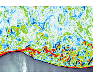
As mentioned before, the airflow measurements over wind-generated surface waves were acquired through a combination of PIV and LIF techniques. The PIV technique was employed to acquire detailed quantitative two-dimensional velocity fields in the air, above the surface waves and within the viscous sublayer, on average as close as  $100~\unicode[STIX]{x03BC}\text{m}$ to the air–water interface. The details of the experimental set-up, wind-wave facility, image acquisition and processing procedure are described at length in Buckley (Reference Buckley2015) and Buckley & Veron (Reference Buckley and Veron2016, Reference Buckley and Veron2017); the reader is referred to those publications for further details of the experiments. Here, to put the available data in perspective, an example of the collated raw data collected is shown in figure 2. Figure 2(a) shows an example of the composite PIV/LIF images acquired by the system. It comprises a large-field-of-view LIF image showing the surface waves in the along-wind direction of the channel. In the airflow, two PIV images are stitched together in order to acquire PIV data over a sufficient field of view. Finally, another LIF image (PIV SD) was used to accurately detect the surface, thereby allowing for PIV velocity estimates to be obtained extremely close to the water surface. Figure 2(b) shows the horizontal velocity field estimated with the PIV images and plotted above the large-field-of-view surface.
Table 1. Summary of experimental conditions. The friction and 10 m extrapolated velocities were calculated by fitting the logarithmic part of the mean wind velocity profile ( $R^{2}$ is systematically above 0.998 for all fitted profiles). The peak wave frequencies, $f_{p}$, were obtained from frequency spectra of single point elevation measurements, and other parameters with subscript $p$ were derived by applying linear wave theory. The peak amplitude was estimated using $a_{p}=\sqrt{2}a_{rms}$, in which $a_{rms}$ is the root-mean-square amplitude. It should also be noted that the data presented here are a re-analysis of the existing raw data acquired by Buckley & Veron (Reference Buckley and Veron2017).
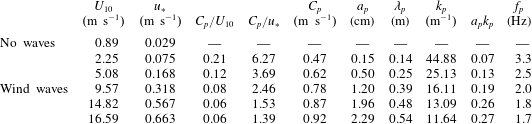

Figure 2. An example of (a) raw composite PIV/LIF image along with the camera’s field of view and (b) estimated horizontal velocity field plotted above the large-field-of-view (LFV) surface. The PIV image, obtained from the concatenation of two side-by-side PIV images with nearly 7.5 % overlap, is plotted over the water portion of the PIV surface detection (SD) image in the large field of view. The PIV SD is used for surface detection within the PIV image. All these images were captured within  $30~\unicode[STIX]{x03BC}\text{s}$. The wind is moving from left to right.
2.2 Coordinate transformation
From the wave elevation detected in the large field of view, we decompose the instantaneous surface into its spatial Fourier components:
 $$\begin{eqnarray}\unicode[STIX]{x1D702}(x)=\mathop{\sum }_{n}^{}a_{n}\text{e}^{\text{i}(k_{n}x+\unicode[STIX]{x1D711}_{n})},\end{eqnarray}$$
 where  $a_{n}$, $k_{n}$ and $\unicode[STIX]{x1D711}_{n}$ are the amplitude, wavenumber and phase of the $n\text{th}$ mode, respectively. A coordinate system that follows the water surface near the interface and tends towards a Cartesian coordinate system farther away from the surface can then be derived. Since higher-order modes of the orbital motion decay away from the surface much faster than lower-order modes, and with the notion that longer waves perturb the airflow up to a higher altitude compared to shorter waves, a wave-following, orthogonal curvilinear coordinate system $(\unicode[STIX]{x1D709}_{1},\unicode[STIX]{x1D709}_{3})=(\unicode[STIX]{x1D709},\unicode[STIX]{x1D701})$ that relates to the Cartesian coordinates $(x_{1},x_{3})=(x,z)$ was defined with the following expressions:
 $$\begin{eqnarray}\left.\begin{array}{@{}c@{}}\displaystyle \unicode[STIX]{x1D709}(x,z)=x-\text{i}\mathop{\sum }_{n}^{}a_{n}\text{e}^{\text{i}(k_{n}x+\unicode[STIX]{x1D711}_{n})}\text{e}^{-k_{n}\unicode[STIX]{x1D701}},\\ \displaystyle \unicode[STIX]{x1D701}(x,z)=z-\mathop{\sum }_{n}^{}a_{n}\text{e}^{\text{i}(k_{n}x+\unicode[STIX]{x1D711}_{n})}\text{e}^{-k_{n}\unicode[STIX]{x1D701}}.\end{array}\right\}\!\end{eqnarray}$$
 A schematic of the decaying wave-following grid is shown in figure 3 for the orthogonal curvilinear coordinate system. The constant  $\unicode[STIX]{x1D701}$-lines are the wave-following lines, and consequently decay towards a horizontal line far away from the water surface. The line $\unicode[STIX]{x1D701}=0$ represents the water surface. Although this type of multi-modal coordinate transformation is now prevalent across numerical studies (e.g. Hara & Sullivan Reference Hara and Sullivan2015), experimental studies, until recently, were unable to report data using such transformations (Buckley & Veron Reference Buckley and Veron2016, Reference Buckley and Veron2017). The velocity components in the Cartesian coordinates $(u_{1},u_{3})=(u,w)$ and orthogonal curvilinear coordinates $(U_{1},U_{3})=(U,W)$ are also represented in figure 3. The flow velocities in the orthogonal curvilinear coordinate system are projections of components of the velocity vector $\boldsymbol{u}$ into the coordinate axes, and are, therefore, in line with the coordinate directions. In a curvilinear coordinate system, physical interpretations of flow-relevant quantities become more intuitive.

Figure 3. Sketch of the decaying wave-following, orthogonal coordinate system along with the velocity components in Cartesian and orthogonal curvilinear coordinates. Here,  $(u_{1},u_{3})=(u,w)$ are components of the velocity vector $\boldsymbol{u}$ in the $(x_{1},x_{3})=(x,z)$ Cartesian coordinates. Equivalently, $(U_{1},U_{3})=(U,W)$ are the velocity components in the $(\unicode[STIX]{x1D709}_{1},\unicode[STIX]{x1D709}_{3})=(\unicode[STIX]{x1D709},\unicode[STIX]{x1D701})$ orthogonal curvilinear coordinate system. The $\unicode[STIX]{x1D701}$ coordinate follows the wave near the surface and tends towards a rectangular coordinate system far away from the surface, outside of the wave boundary layer. The line $\unicode[STIX]{x1D701}=0$ represents the water surface. The constant $\unicode[STIX]{x1D709}$-lines are orthogonal to the constant $\unicode[STIX]{x1D701}$-lines, and, similar to the $\unicode[STIX]{x1D701}$ coordinate, decay towards Cartesian coordinates far away from the surface.
2.3 Wave-turbulence decomposition
In order to study the wave effects on the airflow, it is necessary to separate the mean, wave-induced and turbulent fields. In particular, the separation of waves from the background turbulence has been a persistent challenge over past decades (e.g. Hussain & Reynolds Reference Hussain and Reynolds1970; Lumley & Terray Reference Lumley and Terray1983; Thais & Magnaudet Reference Thais and Magnaudet1995). Depending on wind-wave conditions, various wave separation techniques have been thus far developed for isolating the wave motion. The wave-induced components can be generally obtained by assuming that the turbulence is uncorrelated (linearly) to the periodic motion of the wave (to first order) and statistically stationary. For mechanically generated waves, the wave components can then be extracted by subtracting the ensemble average of a flow quantity from its corresponding phase-averaged variable (e.g. Hussain & Reynolds Reference Hussain and Reynolds1970; Kemp & Simons Reference Kemp and Simons1982; Cheung & Street Reference Cheung and Street1988). The phase-averaging procedure is quite straightforward in the case of monochromatic waves since the instantaneous value of the phase angle is known a priori from the position and phase of the wave-generator paddle. For wind waves, the wave component can be properly isolated based on the assumption of a linear relationship between the wave-induced component and the wave motion at the interface. That is, the wave-induced component is assumed to be coherent with the surface elevation, and thus parts of the variable that does not correlate with the surface displacement are considered to be turbulence (e.g. Benilov, Kouznetsov & Panin Reference Benilov, Kouznetsov and Panin1974; Howe et al. Reference Howe, Chambers, Klotz, Cheung and Street1982; Cheung & Street Reference Cheung and Street1988). For example, Grare et al. (Reference Grare, Lenain and Melville2013a) and Grare, Lenain & Melville (Reference Grare, Lenain and Melville2018) successfully employed Fourier techniques to isolate wave-induced motions, but this spectral approach yields integrated variance and covariances, not the resolved velocity components. Also, these linear correlation techniques include the turbulent components that are correlated with the wave into the wave-induced motions (see Howe et al. Reference Howe, Chambers, Klotz, Cheung and Street1982). In fact, there is no reason to believe that the flow far from the interface (farther than a wavelength say) would correlate substantially with the surface elevation directly beneath the measurements. To address these limitations, Jiang, Street & Klotz (Reference Jiang, Street and Klotz1990) developed a wave separation technique using a nonlinear stream function in which the wave-induced motion can directly interact with turbulence (see also Dean Reference Dean1965). This method was further developed by Thais & Magnaudet (Reference Thais and Magnaudet1995) through combining the linear filtration and potential-solenoidal decomposition techniques in which the wave-induced field is split into an irrotational part and a rotational part. Another powerful method for separating wave components from the background turbulence that was developed specifically for wind waves is based on detecting the wave phases using wave surface profiles, and ensemble averaging the velocities that lie on a vertical line corresponding to a selected phase of the wave. In these cases, since the surface displacement is not strictly monochromatic, the wave phase is generally obtained from geometrical properties of the surface profiles such as zero-crossing, minima (trough) and maxima (crest) of the elevation (e.g. Grare Reference Grare2009; Siddiqui & Loewen Reference Siddiqui and Loewen2010; Birvalski et al. Reference Birvalski, Tummers, Delfos and Henkes2014; Ayati, Vollestad & Jensen Reference Ayati, Vollestad and Jensen2018; Vollestad, Ayati & Jensen Reference Vollestad, Ayati and Jensen2019) and Hilbert transform techniques (e.g. Melville Reference Melville1983; Hristov et al. Reference Hristov, Friehe and Miller1998; Bopp Reference Bopp2018). Siddiqui & Loewen (Reference Siddiqui and Loewen2007) also used a spatial filtering method in which turbulent and wave components were spatially separated based on a cutoff wavenumber that depends on the properties of the coherent structures.
In this paper, we use the wave-phase average of a flow field variable  $\langle f\rangle (\unicode[STIX]{x1D711},\unicode[STIX]{x1D701})$, where $\unicode[STIX]{x1D711}$ is the wave phase, to extract wave-induced velocities and turbulence from the velocity fields. Indeed, an instantaneous flow field variable can be decomposed into the phase-averaged and residual components (Hussain & Reynolds Reference Hussain and Reynolds1970):
 $$\begin{eqnarray}f(\unicode[STIX]{x1D709},\unicode[STIX]{x1D701},t)=\langle f\rangle (\unicode[STIX]{x1D711},\unicode[STIX]{x1D701})+f^{\prime }(\unicode[STIX]{x1D709},\unicode[STIX]{x1D701},t).\end{eqnarray}$$
 The phase-averaged quantity can be further decomposed into the sum of the ensemble mean,  $\bar{f}(\unicode[STIX]{x1D701})$, and wave phase-coherent, $\tilde{f}(\unicode[STIX]{x1D711},\unicode[STIX]{x1D701})$, components, i.e. $\langle f\rangle (\unicode[STIX]{x1D711},\unicode[STIX]{x1D701})=\bar{f}(\unicode[STIX]{x1D701})+\tilde{f}(\unicode[STIX]{x1D711},\unicode[STIX]{x1D701})$. The ensemble mean is thus the average over all phases of the phase-averaged quantities. Assuming that the wave-induced fluctuations are wave-phase coherent, this separation leads to the following so-called triple decomposition of an instantaneous quantity:
 $$\begin{eqnarray}f(\unicode[STIX]{x1D709},\unicode[STIX]{x1D701},t)=\bar{f}(\unicode[STIX]{x1D701})+\tilde{f}(\unicode[STIX]{x1D711},\unicode[STIX]{x1D701})+f^{\prime }(\unicode[STIX]{x1D709},\unicode[STIX]{x1D701},t),\end{eqnarray}$$
 where  $\tilde{f}(\unicode[STIX]{x1D711},\unicode[STIX]{x1D701})$ and $f^{\prime }(\unicode[STIX]{x1D709},\unicode[STIX]{x1D701},t)$ are then considered to be, respectively, the wave-induced and turbulent components. The general properties of the ensemble and phase averages can be found in the reports of Hussain & Reynolds (Reference Hussain and Reynolds1970) and Reynolds & Hussain (Reference Reynolds and Hussain1972) and include
 $$\begin{eqnarray}\overline{f^{\prime }}=0,\quad \langle f^{\prime }\rangle =0,\quad \bar{\tilde{f}}=0,\end{eqnarray}$$
 $$\begin{eqnarray}\overline{\tilde{f}g^{\prime }}=0,\quad \langle \tilde{f}g^{\prime }\rangle =0.\end{eqnarray}$$
 Equations (2.5) simply state that turbulent and wave-induced components have zero means. Equations (2.6) indicate that turbulence does not correlate with the wave-induced fields. We note, however, that while turbulent velocities are not wave correlated, that is not necessarily true for higher-order correlations. In fact, we expect Reynolds stress quantities such as  $\langle U^{\prime }W^{\prime }\rangle$ and $\langle \tilde{U} \tilde{W}\rangle$ to be coherent with the wave phase (see also Thais & Magnaudet (Reference Thais and Magnaudet1995) and Grare (Reference Grare2009) among others).
In the present study, the local instantaneous wave phase was estimated using a Hilbert transform technique (Melville Reference Melville1983; Hristov et al. Reference Hristov, Friehe and Miller1998) applied to the (low-pass-filtered) surface elevation profile obtained from the large-field-of-view LIF image (see Buckley & Veron (Reference Buckley and Veron2017) for details). Low-pass filtering results in a relatively narrow-banded wave signal with 80 % of the waves within periods in the range  $0.8T_{p}$ to $1.2T_{p}$, where $T_{p}$ is the peak wave period. The wave phases were segregated into 144 independent bins, each covering a phase interval of $4.36\times 10^{-2}$ rad. It is also worth mentioning that employing a wave-following coordinate system is necessary for properly defining the mean and phase-averaged variables near the surface, below the highest wave crest. An example of the instantaneous streamwise velocity field along with the decomposed mean, wave-coherent and turbulent residual components for $U_{10}=9.57~\text{m}~\text{s}^{-1}$ is illustrated in figure 4. In figure 4, the instantaneous velocity along $\unicode[STIX]{x1D709}$-axis velocity field, i.e. $U$, is a direct output of the PIV processing as explained in § 2.1. The wave-coherent velocity $\tilde{U}$ is plotted over the corresponding phase of the instantaneous wave surface profiles, and in the Cartesian coordinate system for the purpose of better presentation. Here, for example, the wave-coherent velocity profile at the crest is obtained from averaging all instances of velocity profiles found above the crest of all available instantaneous waves. Moreover, the turbulence is thus defined as the deviation of the instantaneous flow from the corresponding wave-phase average. We note here that since the phase averaging is performed using the phase of the longer peak waves, perturbations to the instantaneous flow induced by short ripples are incorporated in the residual and incorrectly included in the turbulence. Fortunately, these ripples do not contribute substantially to the wavy interface (see figure 1). Furthermore, the influence of these short ripples on the airflow decays exponentially with height above the interface and therefore they do not penetrate the bulk flow. From the difference between the resolved surface profiles and the low passed surface profiles used to determine the phase of the peak waves, we estimate the ripple-induced motion and conclude that our turbulence measurements are at most overestimated by $O(6\,\%)$ at $\unicode[STIX]{x1D701}\approx 0.3~\text{mm}$ from the surface. This ripple-induced contamination drops to less than 1 % for $\unicode[STIX]{x1D701}>1~\text{mm}$.

Figure 4. Example of instantaneous streamwise (along  $\unicode[STIX]{x1D709}$ axis) velocity field along with the decomposed mean, wave-induced and turbulent components for the experiment with a wind speed of $U_{10}=9.57~\text{m}~\text{s}^{-1}$. The first, second, third and fourth columns correspond to the instantaneous, mean, wave-induced and turbulent velocities, respectively. All velocity components are expressed in $\text{m}~\text{s}^{-1}$.
3 Experimental conditions
3.1 Mean flow structure
The mean streamwise velocity profiles are presented in figure 5 for all experimental conditions in the wave-following coordinates and in wall-layer scaled variables, i.e.  $u^{+}=\overline{U}/u_{\ast }$ and $\unicode[STIX]{x1D701}^{+}=\unicode[STIX]{x1D701}u_{\ast }/\unicode[STIX]{x1D708}$ in which $u_{\ast }$ is the friction velocity and $\unicode[STIX]{x1D708}$ is the kinematic viscosity. The mean wind velocity profile above the smooth water surface, when no wave is generated, follows the typical wall-bounded log-law profile as demonstrated in figure 5(a). It clearly exhibits the viscous sublayer near the surface, the buffer (transition) region around $\unicode[STIX]{x1D701}^{+}=10$ and the logarithmic layer. The mean velocity profiles start to deviate from the law of the wall as waves form on the surface (figure 5b). This deviation increases significantly with increasing wind speed and wave slope (see also Hsu & Hsu (Reference Hsu and Hsu1983) and Sullivan et al. (Reference Sullivan, McWilliams and Moeng2000)).

Figure 5. Mean streamwise velocity profiles (a) for smooth water surface, i.e.  $U_{10}=0.89~\text{m}~\text{s}^{-1}$, and (b) for all experimental conditions in the wave-following coordinates and in wall variables $u^{+}=\overline{U}/u_{\ast }$ and $\unicode[STIX]{x1D701}^{+}=\unicode[STIX]{x1D701}u_{\ast }/\unicode[STIX]{x1D708}$. Here, $U$ is the projection of the velocity vector along the $\unicode[STIX]{x1D709}$ coordinate axis. The mean wind velocity profile above the smooth water surface, when no wave is generated, follows the typical wall-bounded log-law profile with a clear viscous sublayer, a buffer layer and a logarithmic region. The extent of the various layers is indicated by vertical dashed lines.
Furthermore, the dimensionless roughness heights  $\unicode[STIX]{x1D701}_{0}^{+}=\unicode[STIX]{x1D701}_{0}u_{\ast }/\unicode[STIX]{x1D708}$, where $\unicode[STIX]{x1D701}_{0}$ is the roughness height, are plotted against the normalized root-mean-square amplitude $a_{rms}^{+}=a_{rms}u_{\ast }/\unicode[STIX]{x1D708}$ in figure 6, where the roughness values are estimated within a fixed frame of reference. Using the definition of the roughness length $\unicode[STIX]{x1D701}_{0}^{+}$, Kitaigorodskii & Donelan (Reference Kitaigorodskii and Donelan1984) categorized the sea surface condition into smooth $\unicode[STIX]{x1D701}_{0}^{+}\lesssim 0.1$, transitional $0.1<\unicode[STIX]{x1D701}_{0}^{+}<2.2$ and rough $\unicode[STIX]{x1D701}_{0}^{+}>2.2$ (see also Donelan Reference Donelan, Le Méhauté and Hanes1990). Based on this classification, the lowest experimental wind speed, $U_{10}=0.89~\text{m}~\text{s}^{-1}$, falls within the smooth flow category, while the experimental conditions with wind speeds of $U_{10}=14.82$ and $16.59~\text{m}~\text{s}^{-1}$ are fully rough. Other experimental conditions, i.e. $U_{10}=2.25,5.08$ and $9.38~\text{m}~\text{s}^{-1}$, are transitionally rough. The water surface and, consequently, the mean flow change from smooth to rough as wind speed increases. Over smooth surfaces, the airflow tends to adhere to the surface, and generally the height of roughness elements is smaller than the viscous sublayer thickness so that the outer flow remains unperturbed. However, when waves appear on the water surface, the airflow becomes transitional as it starts to separate intermittently from the surface. In rough flow conditions, the airflow separates systematically from the steeper waves, and hence the surface roughness increases in such a way that the roughness elements, on average, extend outside the viscous sublayer. Most of the time, the flow over the ocean is transitional or fully rough. The experimental conditions presented in this work also span the surface flow conditions from transitional to fully rough. The corresponding values of the roughness height and dimensionless roughness height are reported in table 2 for all experimental conditions along with the dimensionless values of the viscous sublayer thickness $\unicode[STIX]{x1D6FF}_{0}k_{p}$, where $\unicode[STIX]{x1D6FF}_{0}$ is estimated using $\unicode[STIX]{x1D6FF}_{0}u_{\ast }/\unicode[STIX]{x1D708}=10$ (Phillips Reference Phillips1977). It should be noticed that $\unicode[STIX]{x1D6FF}_{0}k\ll ak$ simply implies that the viscous sublayer thickness is much smaller than the wave amplitude. In the present study (see table 2), the viscous sublayer thickness is smaller than the wave height in all cases, except for the lowest wind speed.

Figure 6. Dimensionless roughness heights  $\unicode[STIX]{x1D701}_{0}^{+}=\unicode[STIX]{x1D701}_{0}u_{\ast }/\unicode[STIX]{x1D708}$ plotted against the normalized root-mean-square amplitude $a_{rms}^{+}=a_{rms}u_{\ast }/\unicode[STIX]{x1D708}$ in a fixed frame of reference. For comparison, the laboratory measurements of Kunishi (Reference Kunishi1963), Hidy & Plate (Reference Hidy and Plate1966) and Banner & Peirson (Reference Banner and Peirson1998) are also presented. The horizontal dashed lines are the limits between smooth, transitional and rough flows based on the classification proposed by Kitaigorodskii & Donelan (Reference Kitaigorodskii and Donelan1984). The solid line is the best log-linear fit to our data.
Table 2. Summary of flow conditions. The dimensionless roughness height was calculated with  $\unicode[STIX]{x1D701}_{0}^{+}=\unicode[STIX]{x1D701}_{0}u_{\ast }/\unicode[STIX]{x1D708}$, where $\unicode[STIX]{x1D701}_{0}$ is the roughness height calculated from the logarithmic law. The viscous sublayer thickness was estimated by $\unicode[STIX]{x1D6FF}_{0}u_{\ast }/\unicode[STIX]{x1D708}=10$ (Phillips Reference Phillips1977). The minimum, maximum and average heights of the critical layer ( $z_{cr}$) from the water surface for all experimental conditions are also reported in the last three columns. The critical height is defined as the height for which the mean airflow velocity matches the phase celerity of the wave, i.e. $\langle U(z_{cr})\rangle -C_{p}=0$. The critical layer height decreases with increasing wind speed. In the lowest wind velocity case, the critical layer did not exist as no waves were formed on the surface.
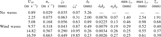

Figure 7. Normalized phase-averaged velocity fields for all experimental conditions. (a–e) Horizontal (along  $\unicode[STIX]{x1D709}$ axis) phase-averaged velocities in a frame of reference moving with the waves, $(\langle U\rangle -C_{p})/U_{10}$. The horizontal velocity fields are shown along with the velocity profiles above the windward side, leeward side, crest and trough of the waves. (f–j) Horizontal (along $\unicode[STIX]{x1D709}$ axis) phase-averaged velocities in which the mean velocities are subtracted, i.e. $(\langle U\rangle -\overline{U})/U_{10}$, in a fixed frame of reference. (k–o) Vertical (along $\unicode[STIX]{x1D701}$ axis) phase-averaged velocities in a fixed frame of reference, $(\langle W\rangle -\overline{W})/U_{10}$, in which, evidently, $\overline{W}=0$. The grey dashed lines indicate the location of the critical layer. The $U$ and $W$ velocity components are illustrated in figure 3.

Figure 8. Normalized horizontal (along  $\unicode[STIX]{x1D709}$ axis) phase-averaged velocities in a frame of reference moving at the wave phase speed, $(\langle U\rangle -C_{p})/U_{10}$, plotted on a logarithmic scale in the wave-following coordinate system for all wind speed cases. The grey dashed lines indicate the location of the critical layer. The airflow below the critical layer is moving in a direction opposite to the main flow, while far from the surface the airflow is in the direction of wave propagation.
3.2 Phase-averaged airflow
The modulations of airflow velocity by the underlying wave motions can be examined through the phase-averaged fields. The horizontal and vertical phase-averaged velocity fields for various experimental conditions are presented in figure 7. In the first column of figure 7, the normalized phase-averaged streamwise velocities are shown in a frame of reference travelling with the peak waves, i.e.  $(\langle U\rangle -C_{p})/U_{10}$. The airflow below the critical layer (Miles Reference Miles1957) is moving in a direction opposite to the main flow, while far from the surface, the airflow travels in the direction of wave propagation. This is particularly clear at the low wind speeds of $U_{10}=2.25~\text{m}~\text{s}^{-1}$ (figure 7a) and $U_{10}=5.08~\text{m}~\text{s}^{-1}$ (figure 7b). The dashed lines in figure 7 indicate the location of the critical layer. The critical layer height decreases with increasing wind speed. In the case of low wind velocity with $U_{10}=2.25~\text{m}~\text{s}^{-1}$, the critical height is, on average, 1.91 mm above the surface and decreases to 0.39 mm for the highest wind speed. The minimum, maximum and average heights of the critical layer for all experiments are summarized in table 2. The critical layer follows the wave undulations quite closely, but with a smaller amplitude. In order to demonstrate the existence of a critical layer in high-wind-speed conditions, the streamwise velocity (in the frame travelling with the waves) is shown on a logarithmic scale in figure 8. It should be emphasized that the critical layer is very close to the surface over young wind waves, and it has therefore been very difficult to detect it experimentally until now. The streamwise velocity fields (figure 7a–e) clearly show the sheltering effect or the streamline asymmetry (Belcher & Hunt Reference Belcher and Hunt1998) in which the airflow accelerates on the windward side of the waves and decelerates on the leeward side. The sheltering effect, in fact, corresponds to the thinning and thickening of the boundary layer as the airflow passes the wave crest. The boundary layer becomes thin (thick) upwind (downwind), which can also be observed in the velocity profiles.
The normalized horizontal (along  $\unicode[STIX]{x1D709}$ axis) phase-averaged velocities with the mean velocities subtracted, i.e. $(\langle U\rangle -\overline{U})/U_{10}$, are presented in figure 7(f–j). The reader should note that these are the so-called wave-induced velocities (denoted with tildes) (e.g. Hsu et al. Reference Hsu, Hsu and Street1981). The normalized horizontal components of the airflow velocity are positive (negative) along the windward (leeward) face of waves and become more intense as wind speed increases. This indicates that the airflow above the critical layer is accelerated on the windward face of the waves and decelerated on the leeward side. In higher winds, the acceleration of the flow is most intense nearly directly above the crest, rather than the windward face of the waves. Below the critical layer, wave-induced velocities are strongly correlated with wave orbital velocities (see Buckley & Veron Reference Buckley and Veron2016). Like the phase-averaged horizontal velocities, the phase-averaged vertical (along $\unicode[STIX]{x1D701}$ axis) velocities also exhibit a phase-locked behaviour, but display an alternating negative–positive pattern along the wave crest (figure 7k–o). While the airflow travels upward above the windward side of the wave crest, and downward above the leeward side, in this coordinate system, $\langle W\rangle$ is negative (positive) on the upwind (downwind) side of waves. This indicates that the mean flow is flatter or less deviated in the $\unicode[STIX]{x1D701}$ direction than the coordinate system $\unicode[STIX]{x1D701}$ lines (i.e. the flow streamlines are flatter than the lines of constant $\unicode[STIX]{x1D701}$). There also exists an asymmetry in the intensity of vertical velocities along the wave crest and particularly near the surface, i.e. the negative velocity on the upwind side of the waves is more intense than its positive counterpart on the downwind side. In the case of low wind velocity with $U_{10}=2.25~\text{m}~\text{s}^{-1}$, the effects of the critical layer are clearly visible. Again, the velocity field within the critical layer suggests that the airflow is strongly affected by the wave surface orbital motions; however, farther above the surface, the airflow is influenced by a sheltering effect past the wave crest.

Figure 9. Instantaneous fields of normalized (a,b) streamwise (along  $\unicode[STIX]{x1D709}$ axis) velocity $U_{1}/U_{10}$, (c,d) horizontal (along $\unicode[STIX]{x1D709}$ axis) turbulent velocity $U_{1}^{\prime }/u_{\ast }$, (e,f) vertical (along $\unicode[STIX]{x1D701}$ axis) turbulent velocity $U_{3}^{\prime }/u_{\ast }$ and (g,h) $\unicode[STIX]{x1D70F}_{t}/\unicode[STIX]{x1D70F}$ over non-separating (a,c,e,g) and separating (b,d,f,h) wind waves for the wind-wave experimental condition of $U_{10}=5.08~\text{m}~\text{s}^{-1}$. The reader is reminded that velocity fields alone are not sufficient to determine the occurrence of separation. Here, we have used the (Galilean-invariant) surface viscous stress to establish airflow separation (see figure 21).
4 Results and discussion
The fully transformed momentum equations for the mean, wave-induced and turbulent fields were derived by Yousefi & Veron (Reference Yousefi and Veron2020) for an orthogonal curvilinear coordinate system. Considering the two-dimensional flow field over wind-generated surface waves, i.e. the current laboratory measurements, the mean momentum equation reduces to
 $$\begin{eqnarray}\displaystyle & & \displaystyle {\displaystyle \frac{1}{h}}{\displaystyle \frac{\unicode[STIX]{x2202}}{\unicode[STIX]{x2202}\unicode[STIX]{x1D709}_{1}}}\left({\displaystyle \frac{h}{h_{1}}}\overline{U}_{1}\overline{U}_{1}\right)+{\displaystyle \frac{1}{h_{3}}}{\displaystyle \frac{\unicode[STIX]{x2202}}{\unicode[STIX]{x2202}\unicode[STIX]{x1D709}_{3}}}\left(\overline{U}_{1}\overline{U}_{3}\right)+{\displaystyle \frac{1}{h_{3}}}{\displaystyle \frac{\unicode[STIX]{x2202}}{\unicode[STIX]{x2202}\unicode[STIX]{x1D709}_{3}}}\left(\overline{\tilde{U} _{1}\tilde{U} _{3}}\right)+{\displaystyle \frac{1}{h_{3}}}{\displaystyle \frac{\unicode[STIX]{x2202}}{\unicode[STIX]{x2202}\unicode[STIX]{x1D709}_{3}}}\left(\overline{U_{1}^{\prime }U_{3}^{\prime }}\right)\nonumber\\ \displaystyle & & \displaystyle \quad =-{\displaystyle \frac{1}{\unicode[STIX]{x1D70C}}}{\displaystyle \frac{1}{h_{1}}}{\displaystyle \frac{\unicode[STIX]{x2202}\bar{p}}{\unicode[STIX]{x2202}\unicode[STIX]{x1D709}_{1}}}+\unicode[STIX]{x1D708}{\displaystyle \frac{1}{h_{3}}}{\displaystyle \frac{1}{h_{3}}}{\displaystyle \frac{\unicode[STIX]{x2202}}{\unicode[STIX]{x2202}\unicode[STIX]{x1D709}_{3}}}\left({\displaystyle \frac{\unicode[STIX]{x2202}\overline{U}_{1}}{\unicode[STIX]{x2202}\unicode[STIX]{x1D709}_{3}}}\right),\end{eqnarray}$$
 where we use the boundary-layer scaling (outlined in Yousefi & Veron (Reference Yousefi and Veron2020)) in which the wave amplitude  $a$ is small compared to the wavelength $\unicode[STIX]{x1D706}=2\unicode[STIX]{x03C0}/k$, and all terms of order $(ak)^{2}$ and higher are neglected. Here, $(\unicode[STIX]{x1D709}_{1},\unicode[STIX]{x1D709}_{3})$ are the orthogonal coordinate axes, $h_{1}$ and $h_{3}$ are the scale factors, $\unicode[STIX]{x1D70C}$ is the density, $\unicode[STIX]{x1D708}$ is the kinematic viscosity and $h=h_{1}h_{3}$. The various terms in (4.1) are presented in detail in the following sections.
4.1 Turbulent stress
In this section, the investigation of the structure of the turbulent stress in the wave boundary layer is detailed. Examples of instantaneous turbulent stress fields, defined as
 $$\begin{eqnarray}\unicode[STIX]{x1D70F}_{t}=-\unicode[STIX]{x1D70C}U_{1}^{\prime }U_{3}^{\prime }\end{eqnarray}$$
 and normalized by the total stress  $\unicode[STIX]{x1D70F}=\unicode[STIX]{x1D70C}u_{\ast }^{2}$, in the airflow are first shown in figure 9 along with the corresponding instantaneous streamwise velocity, streamwise turbulent velocity and vertical turbulent velocity fields over non-separating (left-hand column) and separating (right-hand column) wind waves for the wind-wave experimental condition of $U_{10}=5.08~\text{m}~\text{s}^{-1}$. The separating wave, with a maximum local slope of $\unicode[STIX]{x2202}\unicode[STIX]{x1D702}/\unicode[STIX]{x2202}x=0.31$, has a steeper crest than the non-separating wave, which is smoother and nearly sinusoidal with a local slope of $\unicode[STIX]{x2202}\unicode[STIX]{x1D702}/\unicode[STIX]{x2202}x=0.18$. Instantaneously, the along-surface distribution of the turbulent stress varies substantially over separated and non-separated waves. The turbulent stress is extremely intense on the leeward side of separating waves wherein coherent structures are located in the region of the airflow separation (see figure 9b,d). Just downstream of the wave crest, the airflow detaches from the water surface, and consequently the streamwise turbulent velocity close to the surface falls markedly to a negative value (i.e. the instantaneous velocity is less than the mean flow). Incidentally, the total vertical velocity, because of separation, is nearly zero, leading to a turbulent velocity (i.e. deviation from the mean) that is positive. Thus, in the separated flow region past the wave crest, $U_{1}^{\prime }<0$ and $U_{3}^{\prime }>0$ such that $-U_{1}^{\prime }U_{3}^{\prime }>0$ (see figure 9h). The separated flow region is strongly associated with enhanced turbulent stress. In contrast to the steep wind wave, the turbulent stress past the crest of the non-separating wave showed only a minor increase near the water surface. This slightly increased turbulence is coupled with the ejection of low-velocity fluid from the water surface. The reader is reminded that the turbulent velocities are obtained from subtracting the phase-averaged velocity field from the instantaneous velocities.
The phase-averaged distributions of the normalized turbulent stress,  $\langle \unicode[STIX]{x1D70F}_{t}\rangle /\unicode[STIX]{x1D70F}$, are shown on linear and logarithmic vertical scales in figure 10 for various wind-wave conditions. It can be observed that the turbulent stress presents a phase-locked distribution with the maximum turbulence intensity above the leeward side of the waves. This phase-locked behaviour is consistent with the results of, for example, Yang & Shen (Reference Yang and Shen2010) and Buckley & Veron (Reference Buckley and Veron2016). The intense positive turbulent stress on the leeward side of the waves extends up to $\unicode[STIX]{x1D711}\sim 3\unicode[STIX]{x03C0}/2$ on the windward side of the next wave. The location of the maximum of turbulent stress away from the surface shifts upwind as the wind speed increases; it was located at a phase of $151^{\circ }$, $89^{\circ }$ and $66^{\circ }$ for the 10 m extrapolated wind speeds of 2.25, 5.08 and $9.57~\text{m}~\text{s}^{-1}$, respectively. For the two highest wind speeds, the maximum was located at a phase of $153^{\circ }$ and $146^{\circ }$, respectively. A similar behaviour was observed for the location of the minimum turbulent stress; the minimum of near-zero turbulent stress was located just before the wave crest at a phase of $-9^{\circ }$ for the wind speed of $U_{10}=5.08~\text{m}~\text{s}^{-1}$ and shifts upwind to the phase of $-14^{\circ }$ for the higher wind speeds of $9.57$, $14.82$ and $16.59~\text{m}~\text{s}^{-1}$. For the lowest wind speed, however, the minimum turbulent stress was located slightly on the leeward face of wind wave at a phase of $24^{\circ }$. The general pattern of the turbulent stress for all wind-wave experimental conditions was a peak at roughly the middle of the downwind side of the crest ( $\unicode[STIX]{x1D711}\sim \unicode[STIX]{x03C0}/2$) and a dip just upwind of the crest ( $\unicode[STIX]{x1D711}\sim 0$). It should also be noted that the turbulent stress is substantially reduced below the critical layer height (see figure 10f–j). This can be even observed for the highest wind speeds of $U_{10}=14.82$ and $16.59~\text{m}~\text{s}^{-1}$ from figure 10(i,j). In cases of high wind speed, the distribution of the turbulent stress above the critical layer height presents a pattern of along-wave asymmetry near the surface; the phase-averaged turbulent stress is intense and positive downwind of the crests, and slightly less intense and positive upwind of the crests. The maximum turbulent stress is found downwind of the crest and is certainly enhanced by separation events (see also figure 9). However, separated and non-separated sheltering mechanisms can also lead to increased turbulence downwind of the crest (Belcher & Hunt Reference Belcher and Hunt1993, Reference Belcher and Hunt1998; Belcher, Newley & Hunt Reference Belcher, Newley and Hunt1993). The asymmetry in the positive turbulent stress intensities also correlates with the asymmetry of the mean flow (see figure 7) as well as the mean velocity gradients that cause the acceleration and deceleration of the mean flow on windward and leeward side of waves.

Figure 10. Phase-averaged distribution of the normalized turbulent stress,  $\langle \unicode[STIX]{x1D70F}_{t}\rangle /\unicode[STIX]{x1D70F}$, for different wind speed cases plotted on (a–e) linear and (f–j) logarithmic vertical scales. The linear and logarithmic phase-averaged fields are plotted above the mean water surface as a function of the dimensionless distances $k_{p}z$ and $k_{p}\unicode[STIX]{x1D701}$, respectively. The grey dashed lines indicate the location of the critical layer. The 10 m wind speeds corresponding to each experimental condition are indicated on the left.
The reductions of turbulent stress upstream and about the crest of wind waves are consistent with the assumption that the airflow tends to stabilize and become less turbulent while accelerating upon approaching the wave crest. The action of turbulent stress thickens the boundary layer downwind of the waves resulting in the deceleration of the fluid near the surface. This is in agreement with the results of Belcher & Hunt (Reference Belcher and Hunt1998) that the turbulent stress accelerates (decelerates) the airflow upwind (downwind) of the waves. Furthermore, the varying phase shifts as a function of wind speed are possibly due to the increase in the frequency of separation events with wind speed. In particular, at high wind speeds, the airflow often becomes detached before reaching the wave crest. This is likely caused by the rough surface of the windward side of the wave. This could explain the phase shift of the low-turbulent-stress region towards the upwind direction compared to the case of lowest wind speed. Lastly, it is worth mentioning that the along-wave distribution of turbulent stress becomes more asymmetric about the wave crest closer to the surface. This is partially because the curvature effects are stronger near the surface resulting in a drastic modulation of turbulent stresses due to the presence of surface waves.
The along-wave asymmetry in the turbulent stress was also observed in previous studies (e.g. Belcher et al. Reference Belcher, Newley and Hunt1993; Yang & Shen Reference Yang and Shen2010; Buckley & Veron Reference Buckley and Veron2016). In fact, Buckley & Veron (Reference Buckley and Veron2016) found a difference in sign with a negative–positive pattern of the turbulent stress along the wave crest; the turbulent stress was negative upwind and positive downwind of wave crests (see also Shen et al. (Reference Shen, Zhang, Yue and Triantafyllou2003), Yang & Shen (Reference Yang and Shen2010) and Husain et al. (Reference Husain, Hara, Buckley, Yousefi, Veron and Sullivan2019)). In their study of turbulent flow over a stationary wavy wall, Hudson et al. (Reference Hudson, Dykhno and Hanratty1996) also observed regions of negative turbulent stress upwind of the crests but pointed out that the turbulent stress in a boundary-layer coordinate system assumes positive values everywhere over a wavy wall. Yang & Shen (Reference Yang and Shen2010) also observed regions of negative turbulent stress which they attributed to the negative horizontal gradient of vertical wave-induced motion upwind of the waves. However, our observations suggest that the horizontal wave-induced velocity gradient is too small to substantially affect the turbulence in the wave boundary layer. Since Buckley & Veron (Reference Buckley and Veron2016) found negative–positive values of the turbulent stress  $-\unicode[STIX]{x1D70C}\langle u_{1}^{\prime }u_{3}^{\prime }\rangle$, and our re-analysis of their data finds $-\unicode[STIX]{x1D70C}\langle U_{1}^{\prime }U_{3}^{\prime }\rangle$ positive everywhere above the waves, we infer that the distribution pattern, in particular, the sign of the turbulent stress, is closely dependent on the frame of reference in which the velocity components are defined.
It is important to understand the underlying mechanisms affecting the turbulent momentum exchange across the air–sea interface. The positive turbulent stress (see figure 10) indicates a downward turbulent momentum flux, i.e. the turbulent portion of the momentum is transferred towards the water surface along  $\unicode[STIX]{x1D709}$-lines. The turbulent momentum transfer from the wind to the waves (downward flux) is enhanced on the downwind face of the waves. This is primarily influenced by the separation events and the separated and non-separated sheltering mechanisms. On the windward side of the waves, however, the intermittent bursting events of low-velocity fluid near the surface, which are inherent to wall-bounded turbulent flows (e.g. Kim & Spalart Reference Kim and Spalart1987), are potential candidates for producing positive but less intense turbulent stress. The breakup of ejected streaks of low-speed flow farther above the surface may contribute to the turbulence production on the upwind side of the surface wind waves. The bursting process on the windward side of the waves was also observed by Kawamura & Toba (Reference Kawamura and Toba1988), Yang & Shen (Reference Yang and Shen2010) and others.
To further investigate the turbulent stress in the wave boundary layer, the vertical profiles of the normalized ensemble-averaged turbulent stress,  $\bar{\unicode[STIX]{x1D70F}}_{t}/\unicode[STIX]{x1D70F}$, for different experimental wind speeds are plotted in figure 11. It can be observed that the contribution of the turbulent stress to the total momentum flux increases with wind speed. Moreover, the turbulent stress is reduced within the wave boundary layer possibly because of the wave-induced stress (see § 4.2). This suggests that close to the surface, the work of turbulent stresses on waves is reduced. The turbulent flux is a significant part of the total momentum balance away from the surface. The mean turbulent stress reaches the total stress at a dimensionless distance of approximately $k_{p}\unicode[STIX]{x1D701}=0.5$ for all the experiments. Very close to the surface, the turbulent stress is nearly constant and zero within the viscous sublayer.

Figure 11. Vertical profiles of the mean turbulent stress normalized by the total stress,  $\bar{\unicode[STIX]{x1D70F}}_{t}/\unicode[STIX]{x1D70F}$, for different wind speeds as a function of dimensionless height $k_{p}\unicode[STIX]{x1D701}$. The contribution of turbulent stress to the wind stress increases with wind speed.
4.2 Wave-induced stress
The distributions of the phase-averaged wave-induced stress normalized by the total wind stress,  $\langle \unicode[STIX]{x1D70F}_{w}\rangle /\unicode[STIX]{x1D70F}$, where
 $$\begin{eqnarray}\unicode[STIX]{x1D70F}_{w}=-\unicode[STIX]{x1D70C}\tilde{U} _{1}\tilde{U} _{3}\end{eqnarray}$$
 and  $\unicode[STIX]{x1D70F}=\unicode[STIX]{x1D70C}u_{\ast }^{2}$, are shown on both linear and logarithmic vertical scales for all five wind speed cases in figure 12. Over the four highest wind speeds, there exists an along-wave asymmetry in the positive intensities of the wave-induced stress above the critical height; it is intense and positive on the windward side of wave crests and slightly less intense and positive on the leeward side of wave crests. The regions of positive wave stress (see figure 12b–e,g–j) are intertwined with the areas of negative stress just above the wave crests and downwind of wave troughs. The horizontal position of the negative extremum in the wave stress remains relatively fixed at a phase of $\unicode[STIX]{x03C0}/10$, slightly downwind of wave crests, but its value decreases with wind speed: from $\langle \unicode[STIX]{x1D70F}_{w}\rangle /\unicode[STIX]{x1D70F}=-1.10$ for $U_{10}=5.08~\text{m}~\text{s}^{-1}$ to $\langle \unicode[STIX]{x1D70F}_{w}\rangle /\unicode[STIX]{x1D70F}=-2.17$ for $U_{10}=16.59~\text{m}~\text{s}^{-1}$. The positive wave-induced stress represents momentum transport towards the water surface (downward momentum flux), while the negative stress indicates upward momentum transport. The intense negative-stress region above the critical layer height at the wave crest is partly due to the flow acceleration (deceleration) on the windward (leeward) face of the wave with an intensification of that at the wave crest leading to a strongly positive horizontal wave-induced velocity which means $-\tilde{U} \tilde{W}$ is strongly negative. It was also noted that the vertical wave-induced velocity is slightly positive at the wave crest (see figure 7).

Figure 12. Phase-averaged distribution of the normalized wave-induced stress,  $\langle \unicode[STIX]{x1D70F}_{w}\rangle /\unicode[STIX]{x1D70F}$, for different wind speed cases plotted on (a–e) linear and (f–j) logarithmic vertical scales. The linear and logarithmic phase-averaged fields are plotted above the mean water surface as a function of the dimensionless distances $k_{p}z$ and $k_{p}\unicode[STIX]{x1D701}$, respectively. The grey dashed lines indicate the location of the critical layer. The 10 m wind speeds corresponding to each experimental condition are indicated on the left. The existence of the positive wave-induced stress below the critical layer can be observed even for high-wind-speed conditions.
The wave-induced stress for cases of moderate to high wind speed presents a pattern different from the findings of, for example, Sullivan et al. (Reference Sullivan, McWilliams and Moeng2000) and Buckley & Veron (Reference Buckley and Veron2016) who reported negative wave stress on the upwind and downwind sides of waves. Again, we believe that the difference in the coordinate system used in various studies accounts for these discrepancies. In the wave-following coordinates used here, with the along-axis projected velocities, the vertical wave-induced velocity above the critical height is negative (positive) on the windward (leeward) side of wave crests (see figure 7k–o), which is an opposite trend compared to rectangular coordinates or curvilinear coordinates with rectangular velocities (not shown here). A horizontal wave-induced velocity that forms an along-wave positive–negative pattern about the wave crest (see figure 7f–j) then results in a negative correlation between  $\tilde{U}$ and $\tilde{W}$, i.e. positive wave-induced stress, both upwind and downwind of crests close to the surface. It should also be noted that although the vertical wave-induced velocity in the current study presents a pattern opposite to that of the rectangular coordinates, the horizontal wave-induced velocity is somewhat consistent with its counterpart in rectangular coordinates (its peaks are not necessarily matched) and hence with previous studies (e.g. Sullivan et al. Reference Sullivan, McWilliams and Moeng2000; Kihara et al. Reference Kihara, Hanazaki, Mizuya and Ueda2007; Buckley & Veron Reference Buckley and Veron2016, Reference Buckley and Veron2019).
For the lowest wind speed of  $U_{10}=2.25~\text{m}~\text{s}^{-1}$ (see figure 12a,f), the wave-induced stress field exhibits a pattern different from that of the other cases in that the positive along-wave asymmetry in the intensity of wave-induced stress is considerably less pronounced with its maximum located at the critical height. The position of the positive extremum of the wave stress is shifted downstream compared to the other cases and placed at a phase of approximately $80^{\circ }$. Similar to the high-wind-speed cases, the alternating positive–negative pattern of the wave-induced stress is observed away from the surface, but it has less intensity. Notice that the change of sign across the critical height observed in previous studies (e.g. Hsu et al. Reference Hsu, Hsu and Street1981; Sullivan et al. Reference Sullivan, McWilliams and Moeng2000; Yang & Shen Reference Yang and Shen2010) is presumably an artefact of the Cartesian velocity fields. Here, the wave-induced stress assumes no change across the critical layer. These discrepancies in estimating the wave stress using Cartesian and curvilinear coordinate systems are illustrated in figure 13 for the case of lowest wind speed.

Figure 13. Phase-averaged distribution of the wave-induced stress normalized by the total stress, i.e.  $\langle \unicode[STIX]{x1D70F}_{w}\rangle /\unicode[STIX]{x1D70F}$, calculated using (a) orthogonal curvilinear coordinates $\unicode[STIX]{x1D70F}_{w}=-\unicode[STIX]{x1D70C}\tilde{U} _{1}\tilde{U} _{3}$ and (b) Cartesian coordinates $\unicode[STIX]{x1D70F}_{w}=-\unicode[STIX]{x1D70C}\tilde{u} _{1}\tilde{u} _{3}$ for the lowest wind speed of $U_{10}=2.25~\text{m}~\text{s}^{-1}$. (c) The profiles of the normalized mean wave-induced stress $\bar{\unicode[STIX]{x1D70F}}_{w}/\unicode[STIX]{x1D70F}$. The phase-averaged and mean profile fields are plotted above the mean water surface as a function of the dimensionless distance $k_{p}z$ and $k_{p}\unicode[STIX]{x1D701}$, respectively. The grey dashed lines indicate the location of the critical layer.

Figure 14. Vertical profiles of the mean wave-induced stress normalized by the total stress,  $\bar{\unicode[STIX]{x1D70F}}_{w}/\unicode[STIX]{x1D70F}$, for different wind speeds as a function of the dimensionless height $k_{p}\unicode[STIX]{x1D701}$. Most of the wave stresses are produced close to the surface within the wave boundary layer. For comparison purposes, the results of Hsu et al. (Reference Hsu, Hsu and Street1981) for mechanically generated waves with $U_{10}=2.4~\text{m}~\text{s}^{-1}$ and $C_{p}/u_{\ast }=18.2$ (▫) and Bopp (Reference Bopp2018) for pure wind waves with $U_{10}=12~\text{m}~\text{s}^{-1}$ and $C_{p}/u_{\ast }=1.7$ (○) are also included. We note here that the results of Hsu et al. (Reference Hsu, Hsu and Street1981) are obtained using Cartesian velocities and those of Bopp (Reference Bopp2018) are obtained using the covariance between the horizontal Cartesian and curvilinear-mapped vertical velocities. Therefore, these data should not be considered as an exact comparison with our measurements. Nonetheless, the overall agreement with our data in both amplitude and general vertical variations is good.
Next, figure 14 shows the mean profiles of the wave-induced momentum flux  $\bar{\unicode[STIX]{x1D70F}}_{w}$ scaled by the total wind stress $\unicode[STIX]{x1D70F}$ for all the experimental conditions. The measurements of Hsu et al. (Reference Hsu, Hsu and Street1981) and Bopp (Reference Bopp2018) are also shown for comparison. Most of the wave-induced stresses are produced near the surface within the wave boundary layer, i.e. the height of a wavelength (where $k_{p}\unicode[STIX]{x1D701}=1$). Over the steeper waves with $U_{10}$ of $9.57~\text{m}~\text{s}^{-1}$, for instance, the wave-induced stress is more than 40 % of the total wind flux at the dimensionless height of $k_{p}\unicode[STIX]{x1D701}=0.02$. This contribution reduces over older waves where the wave stress represents 25 % of the total stress at $k_{p}\unicode[STIX]{x1D701}=0.09$ for the lowest wind speed of $2.25~\text{m}~\text{s}^{-1}$. As a general trend, the wave-induced stress decreases to a negative minimum from a near-zero value far from the surface and then increases rapidly to a positive value near the interface. The wave stress, on average, is positive close to the surface representing downward momentum transport and is negative away from the surface representing upward momentum transport. A similar trend but with different peak values was also observed by Sullivan et al. (Reference Sullivan, McWilliams and Moeng2000) and Buckley & Veron (Reference Buckley and Veron2016). Within the wave boundary layer, they respectively found the wave-induced flux to be approximately 20 % and 60 % of the total flux for wave ages of 3.9 and 3.7, while this study estimated the wave-induced flux to contribute almost 45 % to the total flux for the case with wind speed of $5.08~\text{m}~\text{s}^{-1}$ (which corresponds to a wave age of 3.69). This is consistent with the order of magnitude of wave stress in those studies, but details including rate variations and absolute magnitude of wave stress are highly dependent on the frame of reference. Considering figure 14, the maxima of wave-induced stress were observed to occur just above the critical height at approximately $k_{p}\unicode[STIX]{x1D701}=0.02$– $0.035$ over high-wind-speed waves, while for the lowest wind speed, where the effects of the critical layer are appreciable, the maxima were found at a critical height of $k_{p}\unicode[STIX]{x1D701}=0.089$. The minima, however, always occur above the critical height at approximately $k_{p}\unicode[STIX]{x1D701}=0.35$– $0.45$ for all wind speeds. We did not find these extremum points, particularly for the negative minimum farther above the surface, to be consistent with the parameterizations suggested by Hsu & Hsu (Reference Hsu and Hsu1983) based on the length scale of the viscous Stokes layer at the interface. Finally, in comparison with other stress components, it is noted that the wave-induced flux is a substantial portion of the total stress close to the surface (see figure 14) where the turbulent stress is reduced (see figure 11). Far away from the surface, however, the turbulent stress is nearly equal to the total stress, while the wave stress is zero. For all experimental conditions, the wave-induced and turbulent stresses drop to zero very close to the surface, and therefore the stress is supported by the viscosity inside the viscous sublayer (see § 4.4).

Figure 15. (a) The along-wave profiles of wave-induced stress at the height of the critical layer for all the experiments with wind speeds varying from  $2.25$ to $16.59~\text{m}~\text{s}^{-1}$. The profiles are normalized using the total stress $\unicode[STIX]{x1D70F}=\unicode[STIX]{x1D70C}u_{\ast }^{2}$. (b) A sketch of the mean wave shape to visualize the wave phase.
Over wind-driven surface waves, the thin regions below the critical layer are found to be crucial for the exchange of wave-induced momentum between air and water. To more meticulously investigate the wave-induced stress within the critical layer, the phase-averaged distributions of the normalized wave stress are presented in figure 12(f–j), using a logarithmic vertical scale. For the high-wind-speed conditions, the existence of positive wave stress below the critical height can be observed. The patterns of along-wave asymmetry in the positive intensities of the wave-induced stress can also be observed below the critical layer. The magnitude of the positive wave stress at the critical height also decreases with increasing wind speed: they were  $(\bar{\unicode[STIX]{x1D70F}}_{w}/\unicode[STIX]{x1D70F})_{z_{cr}}=0.15$, $0.086$ and $0.082$ for wind speeds of $9.57$, $14.82$ and $16.59~\text{m}~\text{s}^{-1}$, respectively. The along-wave variations of the wave-induced stress at the critical height are further demonstrated in figure 15 for all the experiments conducted in this study. With decreasing wind speed, the magnitude of wave stress increases, and the along-wave profiles of the wave stress depart from the sinusoidal shape observed in the case of highest wind speed and become asymmetric about the wave crest. At the critical height, the peak wave stress is located on the windward side of wave crests (except for the lowest wind speed) and shifts upwind with increasing wind speed: it was located at a phase of $-65^{\circ }$ for a wind speed of $5.08~\text{m}~\text{s}^{-1}$ and at $-80^{\circ }$ for a wind speed of $16.59~\text{m}~\text{s}^{-1}$. For the lowest wind speed, however, the peak wave stress was located on the leeward face of the wave at a phase of approximately $75^{\circ }$. As a general trend, the wave stress is less intense and positive on the leeward side of the waves. Furthermore, the minimum value of wave stress, in contrast to the wave stress away from the surface (see figure 12), was located precisely at wave troughs and reduced as wind speed increased: it was $0.015$, $-0.009$ and $-0.027$ for a wind speed of 2.25, 5.08 and $9.57~\text{m}~\text{s}^{-1}$, respectively. Overall, the wave-induced stress at the critical height dominates the momentum flux in low-wind-speed cases, and its contribution to the total wind stress reduces with increasing wind speed as the critical height moves towards the surface where the viscous stress dominates (see § 4.4). Moreover, the wave stress is larger than the turbulent stress at the critical layer height for all experimental conditions; the contribution of wave-induced stress, on average, was two times greater than that of the turbulent stress at the critical height (not shown here for brevity). Finally, as discussed by Gent & Taylor (Reference Gent and Taylor1977) and further by Sullivan et al. (Reference Sullivan, McWilliams and Moeng2000), the presence of negative (near-surface) wave-induced stress is not a sign of flow separation. In the current study, a detailed examination of the surface wave stress over separating and non-separating wind waves (not presented here) also showed no relation between the negative surface wave-induced stress at the wave crest and the existence of flow separation events.
4.3 Wave-induced turbulent stress
The wave-induced turbulent stress terms, representing the oscillation of the turbulent stress due to the presence of surface waves, are significant not only in the momentum budgets but also in coupling the wave and turbulence fields. The phase-averaged distributions of the wave-induced turbulent stress  $\tilde{r}_{13}$, which is defined as
 $$\begin{eqnarray}\tilde{r}_{13}=\unicode[STIX]{x1D70C}\langle U_{1}^{\prime }U_{3}^{\prime }\rangle -\unicode[STIX]{x1D70C}\overline{U_{1}^{\prime }U_{3}^{\prime }}\end{eqnarray}$$
 normalized by the total wind stress  $\unicode[STIX]{x1D70F}=\unicode[STIX]{x1D70C}u_{\ast }^{2}$, are shown in figure 16 for all the wind-wave experiments conducted in this study. The streamwise-averaged (average across all phases) profiles of the absolute value of $\tilde{r}_{\text{13}}$ fields, i.e. $\overline{|\tilde{r}_{13}|}$, where $|\tilde{r}_{13}|$ is the absolute value, are also plotted in the right-hand panels.

Figure 16. (a–e) Phase-averaged distribution of the wave-induced turbulent stress,  $\tilde{r}_{13}$, along with (f–j) the streamwise-averaged profiles of the absolute value of $\tilde{r}_{13}$ fields, i.e. $\overline{|\tilde{r}_{13}|}$, where $|\tilde{r}_{13}|$ is the absolute value, for all wind-wave experiments. All fields are normalized by the total wind stress. The phase- and streamwise-averaged fields are plotted above the mean water surface as a function of the dimensionless distance $k_{p}z$ and $k_{p}\unicode[STIX]{x1D701}$, respectively. The grey dashed lines indicate the location of the critical layer. The 10 m wind speeds corresponding to each experimental condition are indicated on the left.
In high winds, the distribution of wave-induced turbulent stress forms a positive–negative pattern along the wave crests close to the surface; it is positive (negative) on the windward (leeward) side of the wave crests. This along-wave positive–negative pattern implies that the turbulent stress is relatively high on the leeward side and relatively low on the windward side of the wind-generated waves (see also Hsu et al. (Reference Hsu, Hsu and Street1981) and Hsu & Hsu (Reference Hsu and Hsu1983)). The regions of strong negative wave-induced turbulent stress are found downwind of the waves for all wind speeds, while those with strong positive stress are located approximately at the crest. The negative region, in particular, is highly tilted and extends up to the windward side of the next wave. The airflow separation events past the wave crests are possibly the primary cause of the increased turbulence production downwind of the wind waves. The wave-induced turbulent stress on the leeward face of waves becomes increasingly negative with wind speed. These observations are in qualitative agreement with the simulation results of Kihara et al. (Reference Kihara, Hanazaki, Mizuya and Ueda2007) for slow-moving waves and measurements of Hsu et al. (Reference Hsu, Hsu and Street1981) for fast-moving mechanically generated water waves (see also Hsu & Hsu Reference Hsu and Hsu1983). They showed that  $\tilde{r}_{13}$ is positive (negative) upwind (downwind) of the waves and the minimum (maximum) of $\tilde{r}_{13}$ is located on the downwind (upwind) side of wave crests at a phase of $\unicode[STIX]{x03C0}/2$ ( $3\unicode[STIX]{x03C0}/2$). However, in this study, it was observed that the minimum and maximum of $\tilde{r}_{13}$ occur at a phase of almost $\unicode[STIX]{x03C0}/2$ and $0$, respectively, for the experiment with a wind speed of $U_{10}=5.08~\text{m}~\text{s}^{-1}$. These extrema move upstream with increasing wind speed.
For the lowest wind speed, in general, the turbulence is more uniformly distributed along the wave leading to less turbulence-generating sheltering compared to the larger-amplitude waves. As can be observed from figure 16(a), the positive–negative distribution of  $\tilde{r}_{13}$ along the wave crests and above the critical height now extends below the critical layer. Very close to the surface, however, there exists a layer within which the wave-induced turbulent stress is constant and near zero. The minimum value of $\tilde{r}_{13}$ is shifted downwind and located approximately at the wave trough. The variations of $\overline{|\tilde{r}_{13}|}$ (see figure 16f–j) are large near the water surface and tend to be zero far away from the surface outside the wave boundary layer. Its strength increases as the wind speed increases possibly due to the enhanced separation events. All of the wave-induced turbulent stresses have their maxima above the critical height at about $k_{p}\unicode[STIX]{x1D701}=0.15$– $0.3$.
It is important to note here that, although their peaks are mismatched, the along-wave positive–negative patterns in the wave-induced turbulent stress are not sensitive to the coordinate system. This explains the existence of a qualitative agreement between the current work and the results of Hsu et al. (Reference Hsu, Hsu and Street1981) and Kihara et al. (Reference Kihara, Hanazaki, Mizuya and Ueda2007), while the definition of velocity components are quite different; in their studies, Hsu et al. (Reference Hsu, Hsu and Street1981) and Kihara et al. (Reference Kihara, Hanazaki, Mizuya and Ueda2007) computed the wave-induced turbulent stress in a Cartesian coordinate system, but the present study employed orthogonal curvilinear coordinates. To clarify this, the wave-induced turbulent stresses computed in two different frames of reference, i.e. rectangular and orthogonal curvilinear coordinate systems, over wind waves with  $U_{10}=5.08~\text{m}~\text{s}^{-1}$ close to the surface at a dimensionless distance of $k_{p}\unicode[STIX]{x1D701}=0.065$, are presented in figure 17. This height was chosen because it illustrates large differences between $(\tilde{r}_{UW})_{k_{p}\unicode[STIX]{x1D701}=0.065}$ and $(\tilde{r}_{uw})_{k_{p}\unicode[STIX]{x1D701}=0.065}$ and to make a qualitative comparison with the results of Hsu et al. (Reference Hsu, Hsu and Street1981). The laboratory measurements of Hsu et al. (Reference Hsu, Hsu and Street1981) are for mechanically generated waves with a wave age of 18.2. It is observed that both stress fields vary in a similar manner in that they increase (decrease) windward (leeward) of the crests, but the locations of the maxima are slightly different. Furthermore, they both exhibit marked drops slightly upwind of the wave crests. As a general pattern, they both are positive (negative) upwind (downwind) of wave crests. Similar behaviour is also seen farther above the water surface as well (not shown here). In other words, we find that the wave-induced turbulent stress is weakly influenced by choice of the coordinate system, whereas the wave and turbulent stresses are greatly affected (differences in signs; see §§ 4.1 and 4.2 and figure 13). Therefore, we suggest here that the wave-induced turbulent stress may be a more robust variable to be used for future parameterizations. In all cases, we suggest caution when comparing multiple data sources and results from experimental and/or numerical works since a relatively simple change in coordinate systems lead to marked differences in the turbulent and wave covariances.

Figure 17. (a) Along-wave profiles of the wave-induced turbulent stress computed in two different frames of reference, i.e. rectangular and orthogonal curvilinear coordinate systems, over wind waves with  $U_{10}=5.08~\text{m}~\text{s}^{-1}$ close to the surface at a dimensionless distance of $k_{p}\unicode[STIX]{x1D701}=0.065$. The profiles are normalized using the total stress. (b) A sketch of the mean wave shape to visualize the wave phase. Laboratory measurements by Hsu et al. (Reference Hsu, Hsu and Street1981) for old, mechanically generated waves with a wave age of 18.2 are also plotted for comparison. Both stress fields are positive (negative) upwind (downwind) of the wave crests but with different peaks. Here, $\tilde{r}_{UW}=\unicode[STIX]{x1D70C}\langle U^{\prime }W^{\prime }\rangle -\unicode[STIX]{x1D70C}\overline{U^{\prime }W^{\prime }}$ is computed using the along-axis velocity fields in orthogonal curvilinear coordinates and $\tilde{r}_{uw}=\unicode[STIX]{x1D70C}\langle u^{\prime }w^{\prime }\rangle -\unicode[STIX]{x1D70C}\overline{u^{\prime }w^{\prime }}$ is computed using the velocity fields in Cartesian coordinates.

Figure 18. Phase-averaged distribution of the tangential viscous stress measurements  $\langle \unicode[STIX]{x1D70F}_{\unicode[STIX]{x1D708}}\rangle$ normalized with the total wind stress $\unicode[STIX]{x1D70F}$ for all wind speeds varying from 2.25 to $16.59~\text{m}~\text{s}^{-1}$ plotted on (a–e) linear and (f–j) logarithmic vertical scales. The linear and logarithmic phase-averaged fields are plotted above the mean water surface as a function of the dimensionless distances $k_{p}z$ and $k_{p}\unicode[STIX]{x1D701}$, respectively. The grey dashed lines indicate the location of the critical layer. The 10 m wind speeds corresponding to each experimental condition are indicated on the left.
4.4 Tangential viscous stress
The laboratory measurements of the tangential viscous stress over wind-generated waves, particularly under strong wind forcing conditions, are arguably limited in the literature. The recent works of, for example, Veron et al. (Reference Veron, Saxena and Misra2007) and Grare et al. (Reference Grare, Peirson, Branger, Walker, Giovanangeli and Makin2013b) suggested that viscous stress substantially contributes to the total momentum flux at low wind speeds (see also Banner & Peirson (Reference Banner and Peirson1998) and Peirson & Banner (Reference Peirson and Banner2003)). The phase-averaged distributions of tangential viscous stress measurements  $\langle \unicode[STIX]{x1D70F}_{\unicode[STIX]{x1D708}}\rangle$ are shown on linear and logarithmic vertical scales in figure 18 for all wind speeds varying from 2.25 to $16.59~\text{m}~\text{s}^{-1}$. The tangential viscous stress is computed to leading order in wave slope in the orthogonal curvilinear coordinate system from (Yousefi & Veron Reference Yousefi and Veron2020)
 $$\begin{eqnarray}\unicode[STIX]{x1D70F}_{\unicode[STIX]{x1D708}}=\unicode[STIX]{x1D707}{\displaystyle \frac{1}{h_{3}}}{\displaystyle \frac{\unicode[STIX]{x2202}U_{1}}{\unicode[STIX]{x2202}\unicode[STIX]{x1D709}_{3}}},\end{eqnarray}$$
 where  $\unicode[STIX]{x1D707}$ is the dynamic viscosity of air and $h_{3}$ is the scale factor of the orthogonal coordinate system. All fields are normalized by the total stress $\unicode[STIX]{x1D70F}=\unicode[STIX]{x1D70C}u_{\ast }^{2}$. The phase-averaged distributions of viscous stress present a pattern of along-wave asymmetry near the surface; the stress is highest upwind of the wave crest with its peak value about the crest, and a minimum in the middle of the leeward side of the wave. The maxima of the viscous stress decrease and move downstream with increasing wind speed; the peak of $\langle \unicode[STIX]{x1D70F}_{\unicode[STIX]{x1D708}}\rangle /\unicode[STIX]{x1D70F}=1.03$ occurred at $\unicode[STIX]{x1D711}\approx -55^{\circ }$ for the lowest wind speed and it decreased to $\langle \unicode[STIX]{x1D70F}_{\unicode[STIX]{x1D708}}\rangle /\unicode[STIX]{x1D70F}=0.20$ at $\unicode[STIX]{x1D711}\approx -20^{\circ }$ for the highest wind speed. The phase-locked variations in viscous stress between the wave crest and trough, which increase with wind speed, have the potential to contribute to wave growth. However, far from the surface (at a height of $k_{p}\unicode[STIX]{x1D701}\approx 0.3$ for the lowest wind speed down to $k_{p}\unicode[STIX]{x1D701}\approx 0.1$ for other cases), the viscous tangential stress quickly drops to zero, and the effects of viscosity rapidly become negligible. Very close to the surface at a height of $k_{p}\unicode[STIX]{x1D701}\approx 0.001$, the contribution of the viscous stress to the total momentum flux is significant, particularly for low to moderate wind speeds where, for example, $\overline{\langle \unicode[STIX]{x1D70F}_{\unicode[STIX]{x1D708}}\rangle /\unicode[STIX]{x1D70F}}=0.81$ for $U_{10}=2.25~\text{m}~\text{s}^{-1}$. This contribution decreases with increasing wind speed and drops to $\overline{\langle \unicode[STIX]{x1D70F}_{\unicode[STIX]{x1D708}}\rangle /\unicode[STIX]{x1D70F}}=0.11$ for $U_{10}=16.59~\text{m}~\text{s}^{-1}$. This is consistent with, for example, Banner & Peirson (Reference Banner and Peirson1998), Veron et al. (Reference Veron, Saxena and Misra2007) and Peirson et al. (Reference Peirson, Walker and Banner2014) who also observed that the viscous stress remains an important portion of the total wind stress at moderate wind speeds.
Figure 19 offers a closer look at the viscous stress profiles near the interface and shows the results in the wall-layer coordinates. The critical layer height is indicated with cross symbols for each experiment. Moreover, the results from Hsu et al. (Reference Hsu, Hsu and Street1981) and Bopp (Reference Bopp2018) are presented for comparison. The constant behaviour of the viscous stress profiles is present in all experiments, even for the two high wind speeds of 14.82 and  $16.59~\text{m}~\text{s}^{-1}$, very close to the water surface. The height of this constant layer increases from $\unicode[STIX]{x1D701}^{+}$ of almost $2$ for the lowest wind speed to $\unicode[STIX]{x1D701}^{+}$ of approximately $20$ for the highest wind speed. Above this constant layer, the profiles of the viscous stress smoothly transition into the turbulent region. This transition region contracts quickly as the wind speed increases. Viscous stress profiles collapse to zero with increasing the dimensionless law-of-the-wall distance from the surface. For the lowest wind speed, the viscous tangential stress contributes more than 80 % to the total stress at the surface and remains a significant proportion of the total stress up to $\unicode[STIX]{x1D701}^{+}$ of approximately 20. Although the viscous stress decreases with wind speed, it is still more than 35 % of the total wind stress for wind speed $U_{10}=9.57~\text{m}~\text{s}^{-1}$. For wind-generated surface waves, the viscous tangential stress thus remains substantial into moderate-wind-speed regimes.

Figure 19. Mean profiles of the normalized viscous tangential stress for different wind speeds as a function of dimensionless law-of-the-wall height on a logarithmic scale. For comparison purposes, the results of Hsu et al. (Reference Hsu, Hsu and Street1981) for mechanically generated waves with  $U_{10}=2.4~\text{m}~\text{s}^{-1}$ and $C_{p}/u_{\ast }=18.2$ (▫) and Bopp (Reference Bopp2018) for pure wind waves with $U_{10}=12~\text{m}~\text{s}^{-1}$ and $C_{p}/u_{\ast }=1.7$ (○) are included. The location of the mean critical layer is also indicated with cross symbols. For the lowest wind speed, the viscous tangential stress contributes more than 80 % to the total stress at the surface, and it remains a considerable proportion of the total stress of about 15 % for the high wind speed of $14.82~\text{m}~\text{s}^{-1}$.
The behaviour of the surface tangential viscous stress (the first value of viscous stress measurements taken at a height of  $94.8~\unicode[STIX]{x03BC}\text{m}$ above the air–water interface, denoted here as $\bar{\unicode[STIX]{x1D70F}}_{\unicode[STIX]{x1D708}}^{o}$) is presented in figure 20 as a function of friction velocity. The results from other studies are also shown. Over wind waves, the surface viscous stress increases linearly with friction velocity and then reaches saturation for $u_{\ast }$ above ${\sim}0.4~\text{m}~\text{s}^{-1}$. This unexpected trend manifests at a viscous stress of approximately 0.06 Pa, which is in good agreement with the results of Banner & Peirson (Reference Banner and Peirson1998) and Bopp (Reference Bopp2018) but with a slightly lower saturated value possibly due to different fetches. Airflow separation is a potential candidate for explaining the mechanism of tangential viscous stress saturation at higher wind speeds. Over separating wind waves, as is shown in figure 21, while the surface viscous stress is at its highest on the windward side of the wave, the airflow separation causes a significant drop in the surface stress at the point of separation. The surface viscous stress then becomes negative on the leeward side and remains approximately zero in the separated region. Past the leeward side of the wave, the surface viscous stress gradually increases to a positive value and recovers up to about 50 % of the total wind stress. Over non-separating wind waves, however, the near-surface viscous stress remains positive everywhere along the wave profile and constitutes a significant portion of the total wind stress, despite being reduced on the downwind face of the waves. The intermittent airflow separation events occur more frequently as wind speed increases and wind waves become steeper. Therefore, at higher wind speeds, a smaller fraction of wave surface profiles is exposed to the viscous sublayer, and hence the viscous stress. This implies that the wind stress at the surface is proportional to the fraction of separating waves in the wave field. A comprehensive study of the effect of airflow separation on the near-surface tangential viscous stress can be found in Buckley et al. (Reference Buckley, Veron and Yousefi2020).

Figure 20. Surface tangential viscous stress,  $\bar{\unicode[STIX]{x1D70F}}_{\unicode[STIX]{x1D708}}^{o}$, as a function of friction velocity (black circles). Measurements performed by Mastenbroek et al. (Reference Mastenbroek, Makin, Garat and Giovanangeli1996), Banner & Peirson (Reference Banner and Peirson1998), Grare et al. (Reference Grare, Peirson, Branger, Walker, Giovanangeli and Makin2013b), Peirson et al. (Reference Peirson, Walker and Banner2014) and Bopp (Reference Bopp2018) for pure wind waves are also shown. The results of Mastenbroek et al. (Reference Mastenbroek, Makin, Garat and Giovanangeli1996) were derived from the difference between the total stress and the form drag, compiled by Grare et al. (Reference Grare, Peirson, Branger, Walker, Giovanangeli and Makin2013b). The measurements of Banner & Peirson (Reference Banner and Peirson1998) and Peirson et al. (Reference Peirson, Walker and Banner2014) were conducted in water at relatively short fetches. The black dash-dotted line indicates the total wind stress $\unicode[STIX]{x1D70C}u_{\ast }^{2}$.

Figure 21. Fields of (a,b) normalized instantaneous streamwise velocity  $U/U_{10}$ and (c,d) normalized along-wave instantaneous surface viscous stress $\unicode[STIX]{x1D70F}_{\unicode[STIX]{x1D708}}^{o}/\unicode[STIX]{x1D70F}$ (defined in (4.5) and taken at a height of $94.8~\unicode[STIX]{x03BC}\text{m}$ above the air–water interface) over non-separating (a,c) and separating (b,d) wind waves for the wind-wave experimental condition of $U_{10}=5.08~\text{m}~\text{s}^{-1}$. At the location of separation, the surface viscous stress collapses to approximately zero from its peak value at the wave crest and remains insignificant below the separation bubble.

Figure 22. Profiles of momentum budget terms (defined in (4.8)) normalized by the total wind stress and plotted as a function of (a–e) dimensionless height  $k_{p}\unicode[STIX]{x1D701}$ for wind waves with wind speeds varying from $2.25$ to $16.59~\text{m}~\text{s}^{-1}$ and (f) dimensionless law-of-the-wall height $\unicode[STIX]{x1D701}^{+}$ for the case of the smooth water surface (scale shown at the right) with wind speed of $0.89~\text{m}~\text{s}^{-1}$. The heights of the viscous sublayer and critical layer are indicated by grey horizontal solid and dashed lines, respectively.
4.5 Momentum flux budget
In the sections above, we have independently examined the turbulent, wave-induced and viscous stresses in the flow above waves. In order to gain further insight into the wind-wave momentum exchange and its modulation by the existence of surface wind waves, it is useful to examine the momentum flux budget as a whole. To this end, the vertical momentum budget (see (4.1)) for the mean flow can be expressed as
 $$\begin{eqnarray}\underbrace{{\displaystyle \frac{1}{h_{3}}}{\displaystyle \frac{\unicode[STIX]{x2202}}{\unicode[STIX]{x2202}\unicode[STIX]{x1D709}_{3}}}(\unicode[STIX]{x1D70C}\overline{\tilde{U} _{1}\tilde{U} _{3}})}_{A_{w}}+\underbrace{{\displaystyle \frac{1}{h_{3}}}{\displaystyle \frac{\unicode[STIX]{x2202}}{\unicode[STIX]{x2202}\unicode[STIX]{x1D709}_{3}}}(\unicode[STIX]{x1D70C}\overline{U_{1}^{\prime }U_{3}^{\prime }})}_{A_{t}}-\underbrace{{\displaystyle \frac{1}{h_{3}}}{\displaystyle \frac{1}{h_{3}}}{\displaystyle \frac{\unicode[STIX]{x2202}}{\unicode[STIX]{x2202}\unicode[STIX]{x1D709}_{3}}}\left(\unicode[STIX]{x1D707}{\displaystyle \frac{\unicode[STIX]{x2202}\overline{U}_{1}}{\unicode[STIX]{x2202}\unicode[STIX]{x1D709}_{3}}}\right)}_{D_{\unicode[STIX]{x1D708}}}=-\underbrace{{\displaystyle \frac{1}{h_{1}}}{\displaystyle \frac{\unicode[STIX]{x2202}\bar{p}}{\unicode[STIX]{x2202}\unicode[STIX]{x1D709}_{1}}}}_{P}.\end{eqnarray}$$
 In (4.6),  $A_{w}$ is the advection of momentum by the wave-induced motion, $A_{t}$ is the advection of momentum due to the turbulence fluctuations, $D_{\unicode[STIX]{x1D708}}$ is the viscous diffusion term (or equivalently the stress due to viscosity) and $P$ is the mean horizontal pressure gradient. Indeed, the terms $A_{w}$ and $A_{t}$ represent the flux of (the $\unicode[STIX]{x1D709}_{1}$ component of the) wave-induced and turbulent momentums in the $\unicode[STIX]{x1D709}_{3}$ direction due to the wave and turbulent velocities, respectively. To obtain (4.6), it should be noticed that $\overline{U}_{3}=0$, i.e. the ensemble average of the vertical (along $\unicode[STIX]{x1D709}_{3}$ axis) velocity is zero. In general, however, the mean vertical velocity in a Cartesian coordinate system is a non-zero value, i.e. $\overline{u}_{3}\neq 0$; for example, when the surface drift current is larger in the upwind face of the wave than in the downwind face then $\overline{u}_{3}>0$ at the surface (see also the discussion in Hara & Sullivan (Reference Hara and Sullivan2015)). In addition, in the curvilinear coordinate system adopted here, $\overline{U}_{1}$ is a function of $\unicode[STIX]{x1D709}_{3}$ only.
In a first step, we write (4.6) as
 $$\begin{eqnarray}\left.\begin{array}{@{}c@{}}{\displaystyle \frac{1}{h_{3}}}{\displaystyle \frac{\unicode[STIX]{x2202}}{\unicode[STIX]{x2202}\unicode[STIX]{x1D709}_{3}}}\left(-\unicode[STIX]{x1D70C}\overline{\tilde{U} _{1}\tilde{U} _{3}}-\unicode[STIX]{x1D70C}\overline{U_{1}^{\prime }U_{3}^{\prime }}+\unicode[STIX]{x1D707}{\displaystyle \frac{1}{h_{3}}}{\displaystyle \frac{\unicode[STIX]{x2202}\overline{U}_{1}}{\unicode[STIX]{x2202}\unicode[STIX]{x1D709}_{3}}}\right)={\displaystyle \frac{1}{h_{1}}}{\displaystyle \frac{\unicode[STIX]{x2202}\bar{p}}{\unicode[STIX]{x2202}\unicode[STIX]{x1D709}_{1}}}\\[10.0pt] {\displaystyle \frac{1}{h_{3}}}{\displaystyle \frac{\unicode[STIX]{x2202}}{\unicode[STIX]{x2202}\unicode[STIX]{x1D709}_{3}}}\left(\bar{\unicode[STIX]{x1D70F}}_{w}+\bar{\unicode[STIX]{x1D70F}}_{t}+\bar{\unicode[STIX]{x1D70F}}_{\unicode[STIX]{x1D708}}\right)={\displaystyle \frac{1}{h_{1}}}{\displaystyle \frac{\unicode[STIX]{x2202}\bar{p}}{\unicode[STIX]{x2202}\unicode[STIX]{x1D709}_{1}}},\end{array}\right\}\end{eqnarray}$$
where
 $$\begin{eqnarray}\bar{\unicode[STIX]{x1D70F}}_{w}=-\unicode[STIX]{x1D70C}\overline{\tilde{U} _{1}\tilde{U} _{3}},\quad \bar{\unicode[STIX]{x1D70F}}_{t}=-\unicode[STIX]{x1D70C}\overline{U_{1}^{\prime }U_{3}^{\prime }},\quad \bar{\unicode[STIX]{x1D70F}}_{\unicode[STIX]{x1D708}}=\unicode[STIX]{x1D707}{\displaystyle \frac{1}{h_{3}}}{\displaystyle \frac{\unicode[STIX]{x2202}\overline{U}_{1}}{\unicode[STIX]{x2202}\unicode[STIX]{x1D709}_{3}}}\end{eqnarray}$$
 are the mean wave-induced, turbulent and viscous stresses, respectively. They are shown in figure 22 for all experimental conditions including the case of smooth water surface. All the terms were normalized by the total wind stress  $\unicode[STIX]{x1D70F}=\unicode[STIX]{x1D70C}u_{\ast }^{2}$, and plotted as a function of the dimensionless height $k_{p}\unicode[STIX]{x1D701}$ for experiments with wind surface waves (figure 22a–e) and dimensionless law-of-the-wall height $\unicode[STIX]{x1D701}^{+}$ for the smooth water surface (figure 22f). The heights of the viscous sublayer and critical layer are also indicated by grey horizontal solid and dashed lines, respectively.
Over wind waves, the wave-induced stress largely contributes to the wind stress inside the wave boundary layer. The wave-induced stress decreases to its minimum value from an almost zero value far away from the surface. It then increases to its maximum near the surface. In this region, the turbulent stress decreases monotonically. Close to the surface, the wave stress, at its peak, supports 45 % of the wind stress at a height of  $k_{p}\unicode[STIX]{x1D701}=0.035$ for the wind speed of $5.08~\text{m}~\text{s}^{-1}$, and it decreases to almost 30 % of the wind stress at the height of $k_{p}\unicode[STIX]{x1D701}=0.035$ for wind speeds of $14.89$ and $16.59~\text{m}~\text{s}^{-1}$. In these cases, the maximum wave stress height is considerably above the critical layer height. For the lowest wind speed of $2.25~\text{m}~\text{s}^{-1}$, however, a peak wave stress of 25 % of the wind stress is located at the critical layer height. This is presumably because the effects of the critical layer are stronger in the case of lowest wind speed compared to the other cases. While the turbulent stress is always positive (i.e. downward momentum flux), there exists a region of negative wave stress (i.e. upward momentum flux) farther above the surface between $k_{p}\unicode[STIX]{x1D701}=0.1$ and $k_{p}\unicode[STIX]{x1D701}=1$ for all wind speeds. Elsewhere, the wave stress is positive (i.e. downward momentum flux). For all the experimental conditions, the critical layer height is significantly below the region of negative wave stress. We also note that in negative wave stress regions, the turbulent stress was enhanced, particularly in the higher-wind-speed cases. Closer to the surface, both the wave-induced and turbulent stresses approach zero within the viscous sublayer. The viscous stress is at its largest at the surface, and it becomes negligible farther above the surface. While the contribution of the viscous stress to the total stress decreases with wind stress, it is still approximately 15 % and 10 % of the total stress near the surface for highest wind speeds of $14.82$ and $16.59~\text{m}~\text{s}^{-1}$, respectively.
In contrast, over the flat-water surface, the wave-induced stress is zero throughout the boundary layer, as expected, while the turbulent stress dominates everywhere except within the viscous sublayer where the viscous stress is significant. This compares reasonably with the classical turbulent shear flow over flat surfaces (e.g. Mansour, Kim & Moin Reference Mansour, Kim and Moin1988; Komminaho, Lundbladh & Johansson Reference Komminaho, Lundbladh and Johansson1996). Here, however, a slightly enhanced viscous stress was observed at/near the water surface in which the viscous stress is greater than the total stress,  $\bar{\unicode[STIX]{x1D70F}}_{\unicode[STIX]{x1D708}}>\unicode[STIX]{x1D70F}$. At the height of the viscous sublayer, for example, the turbulent stress is almost 45 % of the total stress and the viscous stress is nearly 65 % of the total stress.
The terms of (4.6) are now plotted in figure 23 as a function of the dimensionless height  $k_{p}\unicode[STIX]{x1D701}$ (figure 23a–e) for the experiment over wind waves and as a function of wall-layer height variable $\unicode[STIX]{x1D701}^{+}$ (figure 23f) for the experiment over the smooth water surface, i.e. when no waves are generated. The data are accordingly scaled with $\unicode[STIX]{x1D70F}k_{p}$ (where $\unicode[STIX]{x1D70F}=\unicode[STIX]{x1D70C}u_{\ast }^{2}$ is the total wind stress) for experiments with wind-generated waves and with $\unicode[STIX]{x1D70F}\unicode[STIX]{x1D6FF}_{0}^{-1}$ for the smooth water surface with $U_{10}=0.89~\text{m}~\text{s}^{-1}$.

Figure 23. Profiles of the wave-induced advection ( $A_{w}$), turbulent advection ( $A_{t}$), viscous diffusion ( $D_{\unicode[STIX]{x1D708}}$) and pressure gradient ( $P$) terms in the momentum flux, defined in (4.6), for wind speeds varying from 0.89 to $16.59~\text{m}~\text{s}^{-1}$. The flux terms are normalized by $\unicode[STIX]{x1D70F}k_{p}$ and plotted as a function of $k_{p}\unicode[STIX]{x1D701}$ for experiments with wind waves (a–e) and they are normalized by $\unicode[STIX]{x1D70F}\unicode[STIX]{x1D6FF}_{0}^{-1}$ and plotted as a function of $\unicode[STIX]{x1D701}^{+}$ (scale shown at the right) for the experiment over the smooth water surface (f). The heights of the viscous sublayer and critical layer are indicated by grey horizontal solid and dashed lines, respectively.

Figure 24. Vertical profiles of the normalized viscous diffusion term,  $D_{\unicode[STIX]{x1D708}}$, for different wind speeds as a function of dimensionless law-of-the-wall height on a logarithmic scale. The profiles of viscous diffusion are normalized by $\unicode[STIX]{x1D70F}\unicode[STIX]{x1D6FF}_{0}^{-1}$. The location of the critical layer is also indicated with crosses.
When waves are present at the surface, the wave-induced advection significantly contributes to the total momentum flux budget, particularly near the surface (see figure 23a–e). It increases to a positive maximum close to the surface at  $k_{p}\unicode[STIX]{x1D701}\approx 0.07$, and then decreases to a negative minimum at the surface. The negative wave-induced advection increases (becomes more negative) as wind speed increases, which indicates that a larger amount of momentum is transported by wave-induced motions towards the water surface. For the lower wind speed of $U_{10}=2.25~\text{m}~\text{s}^{-1}$, the profile of turbulent advection retains a trend broadly similar to that of the smooth water surface but with a larger value at the surface. For other wind-wave conditions, however, the turbulent advection almost decreases exponentially to a negative value at the surface, which increases further in the negative direction with increasing wind speed. In all the cases, the contribution of turbulent advection is smaller than the wave-induced advection term. In all the experimental conditions of this study, the wave-induced advection, turbulent advection and viscous diffusion terms are balanced by the pressure gradient. It should be noticed here that the pressure term is not directly measured in the current study; instead, it is estimated using (4.6).
Evidently, for the smooth water surface (see figure 23f), the momentum flux budget is mainly dominated by the turbulent motion which nearly vanishes above  $\unicode[STIX]{x1D701}_{+}=20$. The turbulent advection term ( $A_{t}$) decreases to a negative peak from an almost zero value far away from the surface and then gradually increases. Closer to the surface approximately below $\unicode[STIX]{x1D701}_{+}=4$, $A_{t}$ remains almost constant. The pressure balances the turbulent advection term at the surface. Moreover, the viscous diffusion term is almost zero everywhere and thus negligible compared to the turbulence.
The viscous diffusion term ( $D_{\unicode[STIX]{x1D708}}$) is noticeably smaller compared to the other terms in the momentum flux budget for all wind speeds. This is because the viscous stress is almost constant within the viscous sublayer and is vanishingly small far away from the surface; therefore, its variations in the vertical direction are rather small except in the viscous–turbulence transition region. In order to carefully examine the viscous diffusion term, the vertical profiles of $D_{\unicode[STIX]{x1D708}}$ are presented in figure 24 and plotted as a function of normalized height in a logarithmic scale. Here, the profiles of viscous diffusion are normalized by $\unicode[STIX]{x1D70F}\unicode[STIX]{x1D6FF}_{0}^{-1}$ and plotted against $\unicode[STIX]{x1D701}^{+}$ for all experimental conditions. Very close to the water surface, the viscous diffusion shows a constant layer for all experimental conditions including the highest wind speed of $16.59~\text{m}~\text{s}^{-1}$. The extent of this layer increases with wind speed; it extends from a dimensionless height of $\unicode[STIX]{x1D701}^{+}\approx 2$ for $U_{10}=2.25~\text{m}~\text{s}^{-1}$ to $\unicode[STIX]{x1D701}^{+}\approx 20$ for $U_{10}=16.59~\text{m}~\text{s}^{-1}$. The general trend is that the diffusion term decreases exponentially to a negative minimum and then linearly increases to a constant value near the surface. Moreover, the contribution of viscous diffusion term (absolute value) in the momentum flux budget decreases with the wind speed. Finally, it should be noticed here that the constant behaviour of viscous diffusion very close to the surface indicates that the viscous stress is not completely constant in this region, but instead there are very slight variations in the viscous stress within the viscous sublayer.
5 Concluding remarks
In this paper, we presented a detailed investigation of the mean, wave-induced and turbulent momentum fluxes in the airflow over wind-generated surface waves. To this end, quantitative airside velocity measurements were obtained in the laboratory over wind-driven surface waves at a fixed fetch and for several forcing conditions corresponding to equivalent 10 m wind speeds ranging from 0.89 to 16.59 m s $^{-1}$. The measurements were obtained using a combined PIV and LIF system described in detail in Buckley & Veron (Reference Buckley and Veron2017). The mean, wave-induced and turbulent velocity fields were extracted from the two-dimensional instantaneous velocity components by means of a linear triple decomposition technique. The wave phase and ensemble averages led to a detailed examination of the role of surface waves in the multiple air–sea momentum fluxes.
Here, we employed an orthogonal wave-following curvilinear coordinate system introduced in the companion study by Yousefi & Veron (Reference Yousefi and Veron2020). This coordinate system was employed for (a) performing the ensemble surface-following averages and extracting the turbulence, (b) the projection of the measured velocity vectors and (c) the expression of the momentum flux terms in the Navier–Stokes equations. While the physics is the same regardless of the frame of reference, we find that the physical interpretation of the observations and the different terms in governing equations is strongly dependent on the frame of reference. A Cartesian system is practical from a laboratory study standpoint and readily allows for differential and spectral analysis (because grid points are evenly distributed and fixed). However, in order to perform horizontal averages, which account for data below wave crests, a surface-following coordinate system is necessary. Hara & Sullivan (Reference Hara and Sullivan2015) used a non-orthogonal coordinate system that is useful for air–sea momentum flux studies. Indeed, using the definition of the wave stress they introduce, the momentum conservation equation is then consistent with the classical constant stress layer (their equation (33)). The curvilinear system employed here is useful for examining flow properties directly at the interface such as, for example, the distribution of the viscous stress along the wavy surface. In that sense, the definition of the surface viscous stress given in (4.5) will appear natural to most readers. We also note that the momentum flux budget given in (4.7) is not substantially more intricate than that obtained by Hara & Sullivan (Reference Hara and Sullivan2015) and also consistent with the constant stress formulation. The curvilinear coordinate system, however, becomes invaluable when performing along-surface averages (as opposed to horizontal averages). In addition, because it is orthogonal, assessing the surface-parallel and surface-normal quantities in such a frame of reference becomes intuitive, and complexities associated with turbulent flows over surface wind waves are easily alleviated. For example, in Cartesian coordinates, the turbulent stress shows negative values near the surface (upwind of wave crests); in the orthogonal curvilinear coordinates, we observed that the turbulent stress assumes positive values everywhere, which is an expected result (e.g. Hudson et al. Reference Hudson, Dykhno and Hanratty1996; Cherukat et al. Reference Cherukat, Na, Hanratty and McLaughlin1998; Calhoun & Street Reference Calhoun and Street2001; Grachev & Fairall Reference Grachev and Fairall2001; Yoon et al. Reference Yoon, El-Samni, Huynh, Chun, Kim, Pham and Park2009). The near-surface negative turbulent stress is a result of the presence of the sloped surface. More simply put, for young waves, there is a vertical component to the wind vector, which is simply due to the flow following the inclined surface. Strictly speaking, the flow is locally parallel to the interface, and  $\boldsymbol{u}=(U,0)$ conveys that fact instinctively. We conclude that the curvilinear frame of reference is particularly useful and facilitates the physical interpretation of the results directly at the air–water interface.
In the first part of this work, §§ 4.1–4.4, we present wave phase-averaged fields in order to examine the along-wave variability of the flow structure. In contrast to the turbulent flows over flat solid boundaries, we observe that the presence of surface waves leads to wave phase-coherent variations in the bulk flow within the so-called wave boundary layer. For example, we find that the phase-averaged turbulent stress is positive everywhere above wind waves, but presents a pattern of along-wave asymmetry close to the surface (approximately  $k_{p}\unicode[STIX]{x1D701}<0.1$) where it is intense and positive downwind of the crests ( ${\sim}0.9\unicode[STIX]{x1D70F}$, on average) and slightly less intense and positive upwind of the crests ( ${\sim}0.6\unicode[STIX]{x1D70F}$, on average). This asymmetry in the positive turbulent stress intensities also correlates with the asymmetry of the mean flow. The maximum of turbulent stress is partly enhanced by separation events downwind of the waves crests. There, the phase-averaged turbulent stress is locally twice the total stress, $\langle \unicode[STIX]{x1D70F}_{t}\rangle /\unicode[STIX]{x1D70F}\approx \mathit{O}(2)$. In contrast, the wave-induced stress, above the critical layer, forms an alternating positive–negative pattern. Close to the interface, however, the wave stress is intense and positive on the windward face of waves ( ${\sim}0.35\unicode[STIX]{x1D70F}$, on average) and slightly less intense and positive on the leeward face of waves ( ${\sim}0.30\unicode[STIX]{x1D70F}$, on average). These positive regions of the wave stress are intertwined with areas of strong negative stress of, on average, about $-0.5\unicode[STIX]{x1D70F}$ just above the wave crests and downwind of wave troughs. At the critical layer height, the contribution of wave-induced stress, on average, is nearly twice that of the turbulent stress, for all experimental conditions. In other words, $\langle \unicode[STIX]{x1D70F}_{w}\rangle _{z_{cr}}/\langle \unicode[STIX]{x1D70F}_{t}\rangle _{z_{cr}}\approx \mathit{O}(2)$. Similarly, the phase averages of the viscous stress (near the surface) also present a pattern of along-wave asymmetry; it is highest on the windward side of the wave, near the crest, and its minimum occurs at the middle of the leeward side of waves. The maxima of the normalized surface viscous stress decrease and shift downstream with increasing wind speed: $\max (\langle \unicode[STIX]{x1D70F}_{\unicode[STIX]{x1D708}}\rangle /\unicode[STIX]{x1D70F})=1.03$ occurs at $\unicode[STIX]{x1D711}\approx -55^{\circ }$ for the lowest wind speed of $U_{10}=2.25~\text{m}~\text{s}^{-1}$ and it decreases to $\max (\langle \unicode[STIX]{x1D70F}_{\unicode[STIX]{x1D708}}\rangle /\unicode[STIX]{x1D70F})=0.20$ located at $\unicode[STIX]{x1D711}\approx -20^{\circ }$ for the highest wind speed of $U_{10}=16.59~\text{m}~\text{s}^{-1}$. Far from the surface, the viscous tangential stress quickly drops to zero at a height of $k_{p}\unicode[STIX]{x1D701}\approx 0.3$ for the lowest wind speed of $U_{10}=2.25~\text{m}~\text{s}^{-1}$ down to $k_{p}\unicode[STIX]{x1D701}\approx 0.1$ for higher wind speeds, and viscous effects rapidly become negligible. Finally, the phase-averaged distribution of the wave-induced turbulent stress is positive (negative) upwind (downwind) of the wave crests. This positive–negative pattern along wave crests implies that the turbulent stress is relatively high on the leeward side and relatively low on the windward side of wind waves. Although the regions of strong negative wave-induced turbulent stress are found downwind of the waves with $\tilde{r}_{13}\approx -0.8\unicode[STIX]{x1D70F}$ ( $-0.35\unicode[STIX]{x1D70F}$ for the lowest wind speed), the positive peaks of $\tilde{r}_{13}\approx \unicode[STIX]{x1D70F}$ ( $0.36\unicode[STIX]{x1D70F}$ for the lowest wind speed) are located approximately at wave crests. The magnitude of these positive peaks is always greater by almost 20 % than that of the negative peaks, that is, $|\!\max (\tilde{r}_{13})|>|\!\min (\tilde{r}_{13})|$. We also found that, in contrast to the turbulent and wave-induced stresses, the general behaviour of the wave-induced turbulent stress is not strongly sensitive to the frame of reference.
In addition to the along-wave phase distributions of the turbulent, wave and viscous stresses, the total momentum flux budget was thoroughly examined (§ 4.5). Far away from the surface and outside the wave boundary layer ( $k_{p}\unicode[STIX]{x1D701}>1$), the turbulent stress dominates the total wind stress such that $\bar{\unicode[STIX]{x1D70F}}_{t}/\unicode[STIX]{x1D70F}\approx 1$, and the wave-induced stress and viscous stress are both negligible. Within the wave boundary layer ( $k_{p}\unicode[STIX]{x1D701}<1$), the wave-induced stress, on average, is positive close to the surface representing downward momentum transport and is negative away from the surface representing upward momentum transport. As a general trend, we find that the mean wave-induced stress decreases to a negative minimum (at $k_{p}\unicode[STIX]{x1D701}$ of approximately 0.35–0.45) from a near-zero value far from the surface. This also corresponds to a maximum turbulent stress. The wave-induced stress then increases rapidly to a positive value near the interface where it supports a substantial portion of the total stress. For example, $\bar{\unicode[STIX]{x1D70F}}_{w}/\unicode[STIX]{x1D70F}\approx 0.4$ at $k_{p}\unicode[STIX]{x1D701}\approx 0.02$ for moderate to high wind speeds. In this region, the turbulent stress is reduced accordingly. Very near the interface, the wave-induced and turbulent stresses are both nearly zero, and therefore the stress is supported by the viscosity within the viscous sublayer. For the lowest wind speed of $U_{10}=2.25~\text{m}~\text{s}^{-1}$, we find that the viscous stress contributes more than 80 % to the total stress at the surface and remains a significant proportion of the total stress (more than 20 %) up to a dimensionless height of $\unicode[STIX]{x1D701}^{+}=20$. Although the normalized viscous stress decreases with wind speed, it is still more than 35 % of the total wind stress at the water interface for a wind speed of $U_{10}=9.57~\text{m}~\text{s}^{-1}$ and approximately 15 % and 10 % of the total wind stress at the surface for the highest wind speeds of $U_{10}=14.82$ and $16.59~\text{m}~\text{s}^{-1}$, respectively. As expected, the viscous stress rapidly falls to zero farther away from the surface in the bulk of the flow such that $\bar{\unicode[STIX]{x1D70F}}_{\unicode[STIX]{x1D708}}<0.05\unicode[STIX]{x1D70F}$ for approximately $\unicode[STIX]{x1D701}^{+}>50$.
Besides providing a detailed view into the physics of the airflow above strongly forced wind waves and offering a comprehensive dataset for comparison with existing and future experimental results (e.g. Grare Reference Grare2009; Bopp Reference Bopp2018), we hope these data will also prove useful in interpreting and/or benchmarking future numerical models (e.g. Sullivan et al. Reference Sullivan, Banner, Morison and Peirson2018; Husain et al. Reference Husain, Hara, Buckley, Yousefi, Veron and Sullivan2019).
Acknowledgements
This research was supported by the National Science Foundation (NSF) through grant numbers OCE-0748767, OCE-1458977 and OCE-1634051. M.P.B. acknowledges support from the National Science Foundation Atmospheric and Geospace Sciences Postdoctoral Research Fellowship AGS-PRF-1524733 and from the Deutsche Forschungsgemeinschaft (DFG, German Research Foundation, project number 274762653, Collaborative Research Centre TRR 181 ‘Energy Transfers in Atmosphere and Ocean’).
Declaration of interests
The authors report no conflict of interest.


 Open access