


1. Introduction
The coupling and interaction of free flow with flows in porous media are ubiquitous. Well-known examples include flows in karst aquifers, hyporheic zones, air or oil filtration, proton-exchange membrane (PEM) fuel cells, as well as blood filtration in the human body. Hence it is important to study the coupled system.
When the flow speed is relatively low (small Reynolds number), the incompressible Stokes system is an excellent model for flow in the free zone (conduit). Time dependency could be included if the temporal evolution is important. Darcy's equation is a well-accepted model for flow in fluid-saturated porous media. Both systems are well-understood, see for example the works of Bear (Reference Bear1988), Tritton (Reference Tritton1988), Batchelor (Reference Batchelor2000) and Temam (Reference Temam2001). The coupling of the two different systems at the interface is of great importance. We will focus on the less controversial case of no-forced filtration. However, there are still genuine disagreements among researchers on what are the ‘correct’ interface boundary conditions even in this case. Continuity of the normal velocity and the pressure are regarded as well-accepted by the fluid dynamics community according to Le Bars & Worster (Reference Le Bars and Worster2006). Nevertheless, the situation with other interfacial conditions is less clear. The second paragraph of the paper by Le Bars & Worster (Reference Le Bars and Worster2006) listed a few competing and sometimes contradicting interfacial conditions such as the Beavers–Joseph (BJ) or its simplification known as the Beavers–Joseph–Saffman–Jones (BJSJ) interface condition, the continuity or discontinuity of the tangential velocity and the continuity or discontinuity of the tangential shear stress among others. See also the works of Ochoa-Tapia & Whitaker (Reference Ochoa-Tapia and Whitaker1995a), Ochoa-Tapia & Whitaker (Reference Ochoa-Tapia and Whitaker1995b), Straughan (Reference Straughan2008) and Zampogna & Bottaro (Reference Zampogna and Bottaro2016). In addition, Eggenweiler & Rybak (Reference Eggenweiler and Rybak2020) and Rybak et al. (Reference Rybak, Schwarzmeier, Eggenweiler and Rüde2020) have provided some evidence on the unsuitability of the BJ interface boundary for filtration problems (It seems that the evidence provided is consistent with the model error introduced by replacing the Stokes system on a perforated domain with the Darcy equation, see for example the work of Shen (Reference Shen2020). The error observed between the microscale model and the macroscale model might be explained in terms of the model error in the porous media without referring to the interfacial conditions.). On the other hand, there are three well-established interface boundary conditions within the mathematics community (Discacciati, Miglio & Quarteroni Reference Discacciati, Miglio and Quarteroni2002; Layton, Schieweck & Yotov Reference Layton, Schieweck and Yotov2002) for the no-forced-filtration case: (i) the continuity of the normal velocity representing the conservation of mass; (ii) the linear balance of forces normal to the interface; and (iii) the BJSJ interface boundary condition. See the next section for more info. These interfacial conditions lead to the mathematical notion of ‘well-posedness’ of the coupled Stokes–Darcy system in the sense that for given reasonable data, there exists one and only one solution, and the solution depends on the data in a continuous fashion (small change to data leads to small change to the solution). The BJSJ interface boundary condition is a heuristic simplification of the original BJ interface boundary condition, which postulates that the tangential component of the normal stress in the free zone (conduit) at the interface is proportional to the jump in tangential velocity across the interface (Beavers & Joseph Reference Beavers and Joseph1967). Beavers and Joseph's work is empirical, and the well-posedness, i.e. the existence and uniqueness of solution to the coupled Stokes–Darcy equations with the BJ condition has not been well-understood. (See the paper by Cao et al. (Reference Cao, Gunzburger, Hua and Wang2010) for a related result.) It seems that two of the interfacial conditions are widely used by both the fluid dynamics and the mathematics communities: (i) the continuity of normal velocity across the interface, and (ii) the BJSJ interface condition. However, the two communities differ on the other interfacial condition. While the fluid dynamics and the groundwater studies communities adopt the continuity of pressure, the mathematics community embraces the balance of the forces normal to the interface, which implies the discontinuity of the pressure across the interface. Hence, there is a genuine need to clarify the relationship between different interfacial boundary conditions, even in this no-forced-filtration case.
Owing to the practical importance of the coupled problem, a lot of effort has been devoted to the development of accurate and efficient numerical methods for the coupled Stokes–Darcy system. See for example the papers by Discacciati et al. (Reference Discacciati, Miglio and Quarteroni2002), Layton et al. (Reference Layton, Schieweck and Yotov2002), Discacciati & Quarteroni (Reference Discacciati and Quarteroni2003), Chen et al. (Reference Chen, Gunzburger, Hua and Wang2011), Chen et al. (Reference Chen, Gunzburger, Sun and Wang2013), Chen et al. (Reference Chen, Gunzburger, Sun and Wang2016) and Ervin et al. (Reference Ervin, Kubacki, Layton, Moraiti, Si and Trenchea2018), the survey paper by Discacciati & Quarteroni (Reference Discacciati and Quarteroni2009), the monograph by Wilbrandt (Reference Wilbrandt2019), and the references therein for works from the mathematical side. A natural idea for efficiency is to design decoupled algorithms so that only one of the subproblems needs to be solved at each time step or iteration. The convergence and long-time stability of these decoupled schemes usually involve a stringent time step constraint for physically relevant small permeability (or hydraulic conductivity). On the other hand, some researchers in the groundwater studies community take a much simpler direct decomposition approach in the numerical simulation: one first solves the free flow problem (Stokes equation) with the no-slip boundary condition on the interface between the free zone (conduit, pure fluid region) and the porous media, followed by solving Darcy's equation with the pressure on the interface prescribed by the pressure of the solution of the Stokes problem on the interface, see for example the papers by Cardenas & Wilson (Reference Cardenas and Wilson2007), Cardenas & Gooseff (Reference Cardenas and Gooseff2008) and Janssen et al. (Reference Janssen, Cardenas, Sawyer, Dammrich, Krietsch and de Beer2012). The groundwater research community's heuristic semi-decoupled approach is certainly very efficient because it involves the solution of two classical problems at once. A natural question is whether such a direct decoupling is valid. If not, what is the error.
To answer the two questions mentioned above, i.e. the validity of the groundwater research community's heuristic decoupled approach and the relationship between various interfacial boundary conditions, we first demonstrate that the interfacial conditions adopted by the mathematics community can be recovered from the classical Helmholtz minimal dissipation principle as long as appropriate dissipation functions are identified. We then non-dimensionalize the system and look at the physically important parameter regimes for possible simplification. The permeability of many common porous media is small. For example, the permeability of well-sorted sand and gravel is approximately  $10^{-8}M^2$ or smaller (Bear Reference Bear1988). Hence the Darcy number $Da$, which is defined as the ratio of the permeability to the typical length squared, is small for most reasonably sized domains. Therefore, it is of great physical relevance to study the small-Darcy-number asymptotic behaviour of the coupled Stokes–Darcy system.
Starting from the system recovered from the Helmholtz minimal dissipation principle, we discover that at the small-Darcy-number regime the leading order dynamics is exactly the semi-decoupled dynamics proposed by the groundwater studies community. We also discover the following relationships between different interfacial boundary conditions at the small-Darcy-number regime: (i) the continuity of the pressure interface condition adopted by the fluid dynamics and groundwater studies communities in the no-forced-filtration case is the leading order behaviour of the balance of forces normal to the interface condition adopted by the mathematics community, and recovered via the minimal dissipation principle, see Remark 3.2; (ii) the continuity of tangential velocity across the interface is the leading order behaviour of the coupled system while the tangential velocity is discontinuous across the interface in general, but the discontinuity is of the order of the square root of the Darcy number, see Remark 3.3; (iii) Saffman's approximation is valid in the sense that the tangential velocity of the Darcy flow at the interface is of the order of the Darcy number, while the tangential velocity of the free flow is of the order of the square root of the Darcy number, see Remark 3.5.
The rest of the manuscript is organized as follows. In § 2, we present a derivation of the Stokes–Darcy system together with the ‘natural’ interface boundary conditions based on the Helmholtz minimal dissipation principle for the no-forced-filtration case. We then introduce the non-dimensional governing equations together with the boundary and interface conditions. In § 3, we construct approximate solutions via asymptotic expansion in the small parameter Darcy number. In particular, we show that the Stokes equation with the no-slip boundary condition on the interface is the leading order dynamics for the pure fluid region, and Darcy's equation with the pressure on the interface prescribed by the pressure of the Stokes flow governs the leading order behaviour in porous media. The consistency of various interfacial boundary conditions is discussed. A rigorous mathematical proof of the formal asymptotic behaviour on a time scale that is relevant to transport in porous media is included in Appendix A for interested readers.
2. The Stokes–Darcy equations
In this section, we show that the Stokes–Darcy system together with appropriate interface boundary conditions can be recovered from the Helmholtz minimal dissipation principle (Batchelor Reference Batchelor2000) provided we identify appropriate energy dissipation rates. We then present a non-dimensionalized version of the coupled system using the typical velocity and length of the conduit (free zone) and introduce our key small parameter—the Darcy number—together with the other physical non-dimensional parameters.
The Stokes system, the Darcy equation and the BJ interface boundary condition are used to motivate the dissipation functions but not in any other manner. Recall that different systems may enjoy the same energy dissipation rate. Indeed, Fields Medalist Terrence Tao constructed a system closely related to the three-dimensional Navier–Stokes system with the same energy dissipation rate. However, the solution to the modified system blows up in finite time while the same question for the three-dimensional Navier–Stokes equation is one of the seven open questions for a million-dollar Millennium Prize posed by the Clay Mathematics Institute (Tao Reference Tao2015). The rate of energy dissipation may not encapsulate all important features of the system even in the linear case. For example, the Coriolis force does not contribute to energy dissipation in general. Therefore, the recovery of the Stokes system, the Darcy equation and the BJSJ interface condition from the Helmholtz minimal dissipation principle is meaningful. In addition, the balance of the forces normal to the interface is nowhere used in the setup of the dissipation function. Hence it is a truly derived interface condition.
There are a variety of derivations of the Stokes–Darcy system, see for example the paper by Mikelic & Jäger (Reference Mikelic and Jäger2000). In fact, a two-phase version of the Stokes–Darcy system, the Cahn–Hilliard–Stokes–Darcy system, was derived via Onsager's extremum principle by Han, Sun & Wang (Reference Han, Sun and Wang2013) without much justification on the dissipation rate functions. See also the papers by Qian, Wang & Sheng (Reference Qian, Wang and Sheng2006) for a variational derivation of the moving contact line dynamics, and by Wang (Reference Wang2021) for a more general framework dubbed ‘generalized Onsager's extremum principle’. The formal derivation presented here can be made rigorous via saddle point theory. Details will be reported elsewhere.
2.1. The Stokes–Darcy system via Helmholtz's principle
We assume a rectangular domain  $\varOmega = [0,L]\times [0,H]$ for simplicity. The domain $\varOmega$ is split into two disjoint subdomains $\varOmega _{c}$ and $\varOmega _{m}$ by a smooth curved interface $\varGamma$, with $\boldsymbol n$ denoting the unit normal of $\varGamma$ pointing from the conduit $\varOmega _{c}$ (the pure fluid region) to porous media $\varOmega _{m}$, and $\boldsymbol {\tau }$ denoting the unit tangent vector to
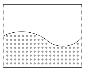
  $\varGamma$. See figure 1 for an illustration. The three-dimensional case can be formulated analogously.

Figure 1. Domian  $\varOmega$.
2.1.1. The time-independent case
Helmholtz's minimal dissipation principle states that for a steady flow in a viscous liquid, with the speeds of flow on the boundaries of the fluid being given as steady and small, the Stokes flow is the one that minimizes the kinetic energy dissipation rate among all incompressible flow configurations (Batchelor Reference Batchelor2000). In other words, the fluid is smart.
Preliminary considerations. Because we are assuming small speeds, both velocities are taken to be incompressible. Hence the normal velocity across the interface  $\varGamma$ between the conduit and the porous media must be continuous to ensure mass conservation, i.e.
 \begin{equation} \boldsymbol{u}_c\cdot{\boldsymbol n} = \boldsymbol{u}_m\cdot{\boldsymbol n}, \end{equation}
where  $\boldsymbol {u}_c$ is the velocity in the conduit while $\boldsymbol {u}_m$ is the Darcy velocity in the porous media.
The rate of energy dissipation functions. To invoke Helmholtz's principle for the recovery of the coupled free flow and porous media flow systems, we identify the rate of kinetic energy dissipation. For the conduit part, the energy dissipation rate is  $\int _{\varOmega _c} 2\eta _0 |\mathbb {D}(\boldsymbol {u}_c)|^2,$ where $\mathbb {D}(\boldsymbol {u}_c)=(\boldsymbol {\nabla } \boldsymbol {u}_c + \boldsymbol {\nabla } \boldsymbol {u}_c^T)/2$ is the rate of deformation tensor and $\eta _0$ is the (constant) viscosity of the fluid (Batchelor Reference Batchelor2000). For the porous media part, the energy dissipation rate is $\int _{\varOmega _m} ({\eta _0}/{\kappa }) |\boldsymbol {u}_m|^2,$ which can be inferred from the time-dependent Darcy equation (Le Bars & Worster Reference Le Bars and Worster2006; Nield & Bejan Reference Nield and Bejan2017). Here the permeability $\kappa$, a tensor in general, is taken to be homogeneous and isotropic, and hence can be represented as a positive constant for the sake of simplicity in our presentation. Our arguments remain valid in the general case as long as the heterogeneity in space is not too strong. Both the Stokes equation and the Darcy equation are used to motivate the rate of the kinetic energy dissipation function. However, their exact forms are not employed here. We reiterate that the rate of energy dissipation may not carry all the information of the underlying model.
Because there is an interface between the conduit and the porous media, additional dissipation on the boundary is possible. Indeed, despite the continuity of the normal velocities, the tangential velocities may contain a gap across the interface  $\varGamma$. In their seminal work (Beavers & Joseph Reference Beavers and Joseph1967), Beavers and Joseph postulated that the viscous fluid exerts a force tangential to the interface (along the interface) that is proportional to the jump in tangential velocity $\boldsymbol {u}_c\cdot \boldsymbol {\tau } -\boldsymbol {u}_m\cdot \boldsymbol {\tau }$ to impede such a jump. A simple dimensional consideration suggests that this force takes the form $-({\alpha _0\eta _0}/{\sqrt {\kappa }})(\boldsymbol {u}_c\cdot \boldsymbol {\tau } -\boldsymbol {u}_m\cdot \boldsymbol {\tau })$, where $\alpha _0$ is a dimensionless number usually determined by experiment. Saffman (Reference Saffman1971) observed that the tangential component of the Darcy velocity at the interface $\varGamma$ is usually much smaller than its free flow counterpart, i.e. $|\boldsymbol {u}_c\cdot \boldsymbol {\tau }| \gg |\boldsymbol {u}_m\cdot \boldsymbol {\tau }|$, hence we may ignore $\boldsymbol {u}_m\cdot \boldsymbol {\tau }$ and approximate the force by $-({\alpha _0\eta _0}/{\sqrt {\kappa }})\boldsymbol {u}_c\cdot \boldsymbol {\tau }$. Therefore, the rate of work done on the interface to dissipate energy is approximately $\int _{\varGamma }({\alpha _0\eta _0}/{\sqrt {\kappa }})|\boldsymbol {u}_c\cdot \boldsymbol {\tau }|^2,$ where we have applied Saffman's simplification a second time.
In summary, the total kinetic energy dissipation rate takes the form:
 \begin{equation} F(\boldsymbol{u}_c,\boldsymbol{u}_m)=\int_{\varOmega_c} 2\eta_0 |\mathbb{D}(\boldsymbol{u}_c)|^2+ \int_{\varOmega_m} \frac{\eta_0}{\kappa} |\boldsymbol{u}_m|^2 +\int_{\varGamma} {\frac{\alpha_0\eta_0}{\sqrt{\kappa}}} |\boldsymbol{u}_{c}\cdot\tau|^2. \end{equation}
 Boundary conditions. A variety of physically relevant boundary conditions are available. For simplicity, we impose a prescribed fluid velocity on  $\varGamma _c$, the boundary of the conduit that is not shared with the porous media. The normal component is set to zero corresponding to no-forced filtration unless periodicity is assumed. And we impose a prescribed zero normal velocity on $\varGamma _m$, the boundary of the porous media not shared with the conduit unless suitable periodicity is stipulated.
The Lagrangian multipliers for the incompressibility constraints. To deal with the incompressibility constraints, we introduce two Lagrange multipliers  $q_c, q_m$ for the incompressibility, and we may formulate Helmholtz's minimal dissipation principle for flows in pure fluid adjacent to porous media by minimizing the following functional:
 \begin{align} {\mathcal{F}}(\boldsymbol{u}_c, q_c, \boldsymbol{u}_m, q_m) &= \int_{\varOmega_c} 2\eta_0 |\mathbb{D}(\boldsymbol{u}_c)|^2- \int_{\varOmega_c} 2q_c \boldsymbol{\nabla}\boldsymbol{\cdot}\boldsymbol{u}_c +\int_{\varGamma} \frac{\alpha_0\eta_0}{\sqrt{\kappa}}|\boldsymbol{u}_c\cdot\boldsymbol{\tau}|^2 \nonumber\\ &\quad + \int_{\varOmega_m} \frac{\eta_0}{\kappa} |\boldsymbol{u}_m|^2 - \int_{\varOmega_m} 2q_m \boldsymbol{\nabla}\boldsymbol{\cdot}\boldsymbol{u}_m, \end{align}
with the boundary conditions specified above plus the mass conservation constraint  $\boldsymbol u_m\cdot \boldsymbol n=\boldsymbol u_c\cdot \boldsymbol n$ on $\varGamma$. This formulation has the advantage that we do not need to deal with the incompressibility constraint explicitly, but through the Lagrange multipliers implicitly.
The derivation. Suppose that  $(\boldsymbol {u}_c, {q}_c, {\boldsymbol {u}}_m, {q}_m)$ is a minimizer of the energy dissipation rate functional $\mathcal {F}$ with the constraint $\boldsymbol u_m\cdot \boldsymbol n=\boldsymbol u_c\cdot \boldsymbol n$ on $\varGamma$. Let $\varphi$ be a smooth function in $\varOmega _c$. Using the fact $(\boldsymbol {u}_c, q_c, \boldsymbol {u}_m, q_m)$ is a minimizer with the constraint $\boldsymbol u_m\cdot \boldsymbol n=\boldsymbol u_c\cdot \boldsymbol n$ on $\varGamma$, we deduce that the function
 \begin{equation} \varPhi_p(s)={\mathcal{F}}(\boldsymbol{u}_c, q_c+s\varphi, \boldsymbol{u}_m, q_m) \end{equation}
must attain its minimum at  $s=0$. Hence, $\varPhi '_p(0)=0$, and we obtain:
 \begin{equation} - \int_{\varOmega_c} 2\varphi \boldsymbol{\nabla}\boldsymbol{\cdot}\boldsymbol{u}_c=0. \end{equation}
The above equation holds for any smooth function  $\varphi$ on $\varOmega _{c}$. Hence we conclude that $\boldsymbol {\nabla }\boldsymbol {\cdot }\boldsymbol {u}_c=0$ in $\varOmega _{c}$. Similarly, $\boldsymbol {\nabla }\boldsymbol {\cdot }\boldsymbol {u}_m=0$ in $\varOmega _{m}$. Therefore, we recover the incompressibility.
Next, we consider perturbation in the velocity field. Let  $\boldsymbol {v}_c$ be a smooth vector field on $\varOmega _c$ that vanishes on $\varGamma _c$, and $\boldsymbol {v}_m$ be a smooth vector field on $\varOmega _m$ satisfying $\boldsymbol {v}_m\cdot \boldsymbol n=0$ on $\varGamma _m$ and $\boldsymbol {v}_c\cdot \boldsymbol n=\boldsymbol {v}_m\cdot \boldsymbol n$ on the interface $\varGamma$. Then the function
 \begin{equation} \varPhi_v(s)={\mathcal{F}}(\boldsymbol{u}_c+s\boldsymbol{v}_c, q_c, \boldsymbol{u}_m+s\boldsymbol{v}_m, q_m) \end{equation}
attains its minimum at  $s=0$ because $\boldsymbol {u}_c+s\boldsymbol {v}_c$ and $\boldsymbol {u}_m+s\boldsymbol {v}_m$ satisfy the specified boundary condition and the continuity of normal velocity constraint, and $(\boldsymbol {u}_c, {q}_c, {\boldsymbol {u}}_m, {q}_m)$ is a minimizer. Hence, $\varPhi '_v(0)=0$, which leads to
 \begin{align} & \int_{\varOmega_{c}}(4\eta_{0}\mathbb{D}(\boldsymbol{u}_{c}):\mathbb{D}(\boldsymbol{v}_c)-2q_c \boldsymbol{\nabla}\boldsymbol{\cdot}{\boldsymbol{v}_c})+ \int_{\varGamma}\frac{\alpha_{0}\eta_{0}}{\sqrt{\kappa}}2(\boldsymbol{u}_{c}\cdot{\boldsymbol\tau}) (\boldsymbol{v}_c\cdot{\boldsymbol\tau}) \nonumber\\ &\quad +\int_{\varOmega_{m}} \left(\frac{\eta_{0}}{\kappa}2\boldsymbol{u}_{m}\cdot\boldsymbol{v}_m-2q_m \boldsymbol{\nabla}\boldsymbol{\cdot}\boldsymbol{v}_m\right)=0. \end{align}
 Because  $\mathbb {D}(\boldsymbol {u}_{c})$ is a symmetric matrix, it follows that $\mathbb {D}(\boldsymbol {u}_{c}):\mathbb {D}(\boldsymbol {v}_c)=\mathbb {D}(\boldsymbol {u}_{c}):\boldsymbol {\nabla }\boldsymbol {v}_c$. After performing integration by parts on the first and last terms on the left-hand side, we deduce
 \begin{align} 0 &=
\int_{\varOmega_{c}}2({-}2\eta_{0}\boldsymbol{\nabla}\boldsymbol{\cdot}\mathbb{D}(\boldsymbol{u}_{c})+\boldsymbol{\nabla}
q_c)\cdot{\boldsymbol{v}_c} \nonumber\\ &\quad +
\int_{\varGamma}\left(4\eta_{0}{\boldsymbol{v}_c}\cdot\mathbb{D}(\boldsymbol{u}_{c}){\boldsymbol
n}
+\frac{\alpha_{0}\eta_{0}}{\sqrt{\kappa}}2(\boldsymbol{u}_{c}\cdot{\boldsymbol\tau})({\boldsymbol{v}_c}\cdot{\boldsymbol\tau})\right)
+\int_\varGamma 2(q_m \boldsymbol{v}_m\cdot\boldsymbol n -
q_c \boldsymbol{v}_c\cdot\boldsymbol n) \nonumber\\ &\quad
+\int_{\varOmega_{m}}2(\frac{\eta_{0}}{\kappa}\boldsymbol{u}_{m}
+ \boldsymbol{\nabla} q_m )\cdot{\boldsymbol{v}_m}
\nonumber\\ &=
\int_{\varOmega_{c}}2({-}2\eta_{0}\boldsymbol{\nabla}\boldsymbol{\cdot}\mathbb{D}(\boldsymbol{u}_{c})+\boldsymbol{\nabla}
q_c)\cdot{\boldsymbol{v}_c} +
\int_{\varGamma}2(2\eta_{0}\boldsymbol
n\cdot\mathbb{D}(\boldsymbol{u}_{c}){\boldsymbol n}
-q_c+q_m)\boldsymbol{v}_c\cdot\boldsymbol n \nonumber\\
&\quad
+\int_{\varGamma}2(2\eta_{0}{\boldsymbol\tau}\cdot\mathbb{D}(\boldsymbol{u}_{c}){\boldsymbol
n}
+\frac{\alpha_{0}\eta_{0}}{\sqrt{\kappa}}\boldsymbol{u}_{c}\cdot{\boldsymbol\tau})({\boldsymbol{v}_c}\cdot{\boldsymbol\tau})
+\int_{\varOmega_{m}}2\left(\frac{\eta_{0}}{\kappa}\boldsymbol{u}_{m}
+ \boldsymbol{\nabla} q_m \right)\cdot{\boldsymbol{v}_m},
\end{align}
\begin{align} 0 &=
\int_{\varOmega_{c}}2({-}2\eta_{0}\boldsymbol{\nabla}\boldsymbol{\cdot}\mathbb{D}(\boldsymbol{u}_{c})+\boldsymbol{\nabla}
q_c)\cdot{\boldsymbol{v}_c} \nonumber\\ &\quad +
\int_{\varGamma}\left(4\eta_{0}{\boldsymbol{v}_c}\cdot\mathbb{D}(\boldsymbol{u}_{c}){\boldsymbol
n}
+\frac{\alpha_{0}\eta_{0}}{\sqrt{\kappa}}2(\boldsymbol{u}_{c}\cdot{\boldsymbol\tau})({\boldsymbol{v}_c}\cdot{\boldsymbol\tau})\right)
+\int_\varGamma 2(q_m \boldsymbol{v}_m\cdot\boldsymbol n -
q_c \boldsymbol{v}_c\cdot\boldsymbol n) \nonumber\\ &\quad
+\int_{\varOmega_{m}}2(\frac{\eta_{0}}{\kappa}\boldsymbol{u}_{m}
+ \boldsymbol{\nabla} q_m )\cdot{\boldsymbol{v}_m}
\nonumber\\ &=
\int_{\varOmega_{c}}2({-}2\eta_{0}\boldsymbol{\nabla}\boldsymbol{\cdot}\mathbb{D}(\boldsymbol{u}_{c})+\boldsymbol{\nabla}
q_c)\cdot{\boldsymbol{v}_c} +
\int_{\varGamma}2(2\eta_{0}\boldsymbol
n\cdot\mathbb{D}(\boldsymbol{u}_{c}){\boldsymbol n}
-q_c+q_m)\boldsymbol{v}_c\cdot\boldsymbol n \nonumber\\
&\quad
+\int_{\varGamma}2(2\eta_{0}{\boldsymbol\tau}\cdot\mathbb{D}(\boldsymbol{u}_{c}){\boldsymbol
n}
+\frac{\alpha_{0}\eta_{0}}{\sqrt{\kappa}}\boldsymbol{u}_{c}\cdot{\boldsymbol\tau})({\boldsymbol{v}_c}\cdot{\boldsymbol\tau})
+\int_{\varOmega_{m}}2\left(\frac{\eta_{0}}{\kappa}\boldsymbol{u}_{m}
+ \boldsymbol{\nabla} q_m \right)\cdot{\boldsymbol{v}_m},
\end{align}
where we have used the continuity of the normal velocity constraint  $\boldsymbol {v}_c\cdot \boldsymbol n=\boldsymbol {v}_m\cdot \boldsymbol n$ on the interface $\varGamma$ in deducing the second term in the last equation.
Setting  $\boldsymbol {v}_m=0$ and choosing $\boldsymbol {v}_c$ with $\boldsymbol {v}_c=0$ on $\varGamma$, we deduce
 \begin{equation} \int_{\varOmega_{c}}({-}2\eta_{0}\boldsymbol{\nabla}\boldsymbol{\cdot}\mathbb{D}(\boldsymbol{u}_{c})+\boldsymbol{\nabla} q_c)\cdot{\boldsymbol{v}_c}=0, \end{equation}
which yields the Stokes equations
 \begin{equation} -2\eta_{0}\boldsymbol{\nabla}\boldsymbol{\cdot}\mathbb{D}(\boldsymbol{u}_{c})+\boldsymbol{\nabla} q_c=0\quad\text{in}\ \varOmega_{c}, \end{equation}
with the Lagrangian multiplier  $q_c$ for the incompressibility in the conduit serving the role of the pressure in the conduit.
Next, we set  $\boldsymbol {v}_c=0$, and we deduce the Darcy equation
 \begin{equation} \frac{\eta_{0}}{\kappa}\boldsymbol{u}_{m}+\boldsymbol{\nabla} q_{m} =0, \end{equation}
with the Lagrangian multiplier  $q_m$ for the incompressibility of the fluid in porous media serving the role of the pressure in porous media.
Hence we are left with
 \begin{align} 0 &= \int_{\varGamma}2(2\eta_{0}\boldsymbol n\cdot\mathbb{D}(\boldsymbol{u}_{c}){\boldsymbol n} -q_c+q_m)\boldsymbol{v}_c\cdot\boldsymbol n \nonumber\\ &\quad +\int_{\varGamma}2\left(2\eta_{0}{\boldsymbol\tau}\cdot\mathbb{D}(\boldsymbol{u}_{c}){\boldsymbol n}+ \frac{\alpha_{0}\eta_{0}}{\sqrt{\kappa}}\boldsymbol{u}_{c}\cdot{\boldsymbol\tau}\right)({\boldsymbol{v}_c}\cdot{\boldsymbol\tau}). \end{align}
Choosing  $\boldsymbol {v}_c$ so that $\boldsymbol {v}_c\cdot \boldsymbol n=0$ on $\varGamma$, we deduce
 \begin{equation} \int_{\varGamma}\left(2\eta_{0}{\boldsymbol\tau}\cdot\mathbb{D}(\boldsymbol{u}_{c}){\boldsymbol n}+ \frac{\alpha_{0}\eta_{0}}{\sqrt{\kappa}}(\boldsymbol{u}_{c}\cdot{\boldsymbol\tau})\right){\boldsymbol{v}_c}\cdot{\boldsymbol\tau}=0. \end{equation}
Because  ${\boldsymbol {v}_c}\cdot {\boldsymbol \tau }$ is arbitrary, from the equation above, we recover the BJSJ interface boundary condition:
 \begin{equation} {\boldsymbol\tau}\cdot\mathbb{T}(\boldsymbol{u}_{c}, q_c){\boldsymbol n}+ \frac{\alpha_{0}\eta_{0}}{\sqrt{\kappa}}\boldsymbol{u}_{c}\cdot{\boldsymbol\tau}=0. \end{equation}
On the other hand, choosing  $\boldsymbol {v}_c$ so that $\boldsymbol {v}_c\cdot {\boldsymbol \tau }=0$ on $\varGamma$, we deduce
 \begin{equation} \int_{\varGamma}(2\eta_{0}\boldsymbol n\cdot\mathbb{D}(\boldsymbol{u}_{c}){\boldsymbol n} -q_c+q_m)\boldsymbol{v}_c\cdot\boldsymbol n=0. \end{equation}
This implies the balance of forces normal to the interface because  $\boldsymbol {v}_c\cdot \boldsymbol n$ can be an arbitrary function,
 \begin{equation} \boldsymbol n\cdot\mathbb{T}(\boldsymbol{u}_c,q_c)\boldsymbol n ={-}q_m. \end{equation}
Summary. To summarize, we have derived the following Euler–Lagrange equations satisfied by the minimizer,
 $$\begin{gather} -2\eta_0\boldsymbol{\nabla}\boldsymbol{\cdot}\mathbb{D}(\boldsymbol{u}_c) + \boldsymbol{\nabla} q_c = 0,\quad \boldsymbol{\nabla}\boldsymbol{\cdot}\boldsymbol{u}_c=0,\quad \mbox{in}\ \varOmega_c, \end{gather}$$
 $$\begin{gather}\frac{\eta_0}{\kappa}\boldsymbol{u}_m +\boldsymbol{\nabla} q_m = 0,\quad \boldsymbol{\nabla}\boldsymbol{\cdot}\boldsymbol{u}_m=0, \quad \mbox{in}\ \varOmega_m, \end{gather}$$
 $$\begin{gather}-{\boldsymbol\tau}\cdot \mathbb{T}(\boldsymbol u_c, q_c)\boldsymbol n = \frac{\alpha_0\eta_0}{\sqrt{\kappa}}{\boldsymbol\tau}\cdot\boldsymbol u_c, \quad \mbox{on}\ \varGamma, \end{gather}$$
 $$\begin{gather}-\boldsymbol n\cdot \mathbb{T}(\boldsymbol u_c, q_c)\boldsymbol n =q_m, \quad \mbox{on}\ \varGamma, \end{gather}$$
 $$\begin{gather}\boldsymbol u_c\cdot\boldsymbol n = \boldsymbol u_m\cdot\boldsymbol n, \quad \mbox{on}\ \varGamma. \end{gather}$$
Notice that as the last interfacial boundary condition, the continuity of normal velocity is imposed to ensure mass conservation. We observe that this Euler–Lagrange equation is exactly the classical Stokes–Darcy system with the BJSJ interface boundary condition (2.19) and the balance of the forces normal to the interface boundary condition (2.20), as proposed by Quarteroni and collaborators (Discacciati & Quarteroni Reference Discacciati and Quarteroni2009). The Lagrange multipliers for the incompressibility happen to be the pressures (hence the mathematical saying that ‘the pressure is the Lagrangian multiplier for the incompressibility’). Therefore, we will replace  $q_c, q_m$ by $p_c, p_m$, respectively. Both the BJSJ interface boundary condition and the balance of the force normal to the interface $\varGamma$ appear in the process of this variational manipulation.
Remark 2.1 The presentation above indicates that the BJSJ interface boundary condition is fully consistent with the Helmholtz minimal dissipation principle. This is in accordance with the known fact that BJSJ leads to a well-posed Stokes–Darcy system with unique solution and continuous dependence on data. In contrast, there is no known direct consistency argument between the original BJ interface boundary condition and Helmholtz's minimal dissipation principle. There is no known well-posedness result for the steady Stokes–Darcy system with the original BJ interface boundary condition in general either. All these suggests the BJSJ interfacial boundary condition is more natural from the energetic consideration, and more convenient from the mathematics perspective.
2.1.2. Variational derivation of the case with a source
If there is a source term or external forcing  $\boldsymbol {f}_c$ such as the gravitational force or a pressure gradient in the conduit, we could include an additional term related to the work done by the external forcing and arrive at the following generalized Helmholtz principle:
 \begin{align} {\mathcal{F}}_f(\boldsymbol{u}_c, p_c, \boldsymbol{u}_m, p_m) &= \int_{\varOmega_c} 2\eta_0 |\mathbb{D}(\boldsymbol{u}_c)|^2- \int_{\varOmega_c} 2p_c \boldsymbol{\nabla}\boldsymbol{\cdot}\boldsymbol{u}_c +\int_{\varGamma} \frac{\alpha_0\eta_0}{\sqrt{\kappa}}|\boldsymbol{u}_c\cdot\boldsymbol{\tau}|^2 \nonumber\\ &\quad + \int_{\varOmega_m} \frac{\eta_0}{\kappa} |\boldsymbol{u}_m|^2 - \int_{\varOmega_m} 2p_m \boldsymbol{\nabla}\boldsymbol{\cdot}\boldsymbol{u}_m -2\int_{\varOmega_c}\boldsymbol{f}_c\cdot\boldsymbol{u}_c, \end{align}
subject to the mass conservation constraint  $\boldsymbol u_m\cdot \boldsymbol n=\boldsymbol u_c\cdot \boldsymbol n$ on $\varGamma$.
The same argument as in the previous subsection leads to the corresponding Euler–Lagrange equations for this case:
 $$\begin{gather} -2\eta_0\boldsymbol{\nabla}\boldsymbol{\cdot}\mathbb{D}(\boldsymbol{u}_c) + \boldsymbol{\nabla} p_c = \boldsymbol{f}_c,\quad \boldsymbol{\nabla}\boldsymbol{\cdot}\boldsymbol{u}_c=0,\quad \mbox{in}\ \varOmega_c, \end{gather}$$
 $$\begin{gather}\frac{\eta_0}{\kappa}\boldsymbol{u}_m +\boldsymbol{\nabla} p_m = 0,\quad \boldsymbol{\nabla}\boldsymbol{\cdot}\boldsymbol{u}_m=0, \quad \mbox{in}\ \varOmega_m, \end{gather}$$
together with the same interface coupling conditions (2.19)–(2.21). This is exactly the well-known time-independent (steady-state) Stokes–Darcy system with a source term in the conduit together with the BJSJ interface boundary condition and the balance of normal-force interface boundary condition (Discacciati et al. Reference Discacciati, Miglio and Quarteroni2002; Layton et al. Reference Layton, Schieweck and Yotov2002; Discacciati & Quarteroni Reference Discacciati and Quarteroni2009; Wilbrandt Reference Wilbrandt2019).
2.1.3. The time-dependent case
The time-dependent Stokes–Darcy system with BJSJ interface can be recovered analogously by using the gradient flow idea. The Darcy velocity  $\boldsymbol {u}_m$ (or the pressure in porous media $p_m$) can be viewed as a function of the velocity $\boldsymbol {u}_c$ and the pressure $p_c$ in the conduit. Indeed, we could use (2.20) to solve Darcy's equation together with other appropriate boundary conditions once $\boldsymbol {u}_c$ and $p_c$ are given. In other words, the Darcy velocity is slaved by the Stokes velocity. Hence, we may formulate the objective functional as a functional of the variables in the conduit only and apply the gradient flow framework to come up with the following time-dependent Stokes–Darcy system:
 $$\begin{gather} \rho_0\frac{\partial\boldsymbol{u}_c}{\partial t}-\boldsymbol{\nabla}\boldsymbol{\cdot}\mathbb{T}(\boldsymbol{u}_c, p_c) = \boldsymbol{f}_c,\quad \boldsymbol{\nabla}\boldsymbol{\cdot}\boldsymbol{u}_c=0,\quad \mbox{in}\ \varOmega_c, \end{gather}$$
 $$\begin{gather}\frac{\eta_0}{\kappa}\boldsymbol{u}_m +\boldsymbol{\nabla} p_m = 0,\quad \boldsymbol{\nabla}\boldsymbol{\cdot}\boldsymbol{u}_m=0, \quad \mbox{in}\ \varOmega_m, \end{gather}$$
together with the same interface coupling conditions (2.19)–(2.21).
This is exactly the well-known time-dependent (unsteady-state) Stokes–Darcy system with a source term in the conduit together with the BJSJ interface boundary condition (Discacciati et al. Reference Discacciati, Miglio and Quarteroni2002; Discacciati & Quarteroni Reference Discacciati and Quarteroni2009; Wilbrandt Reference Wilbrandt2019).
Notice that the solution to this system is not unique. Indeed, if  $(\boldsymbol {u}_c, p_c, \boldsymbol {u}_m, p_m)$ is a solution, $(\boldsymbol {u}_c, p_c+C, \boldsymbol {u}_m, p_m+C)$ is also a solution for any constant $C$. To ensure uniqueness of solution, we impose
 \begin{equation} \int_{\varOmega_m} p_m = 0. \end{equation}
This is equivalent to choosing a proper reference frame for the pressure.
2.2. Non-dimensional form
We now derive the non-dimensionalized form of the Stokes–Darcy system using the typical units associated with the free flow.
We use the typical length  $L$, velocity $U_{0}$ and pressure difference $\delta P$ of the free flow in the conduit (pure fluid region) and we introduce the following scalings to non-dimensionalize the Stokes–Darcy system (2.25) and (2.26):
 \begin{equation} \left.\begin{gathered} {\boldsymbol u}_{c} =\widetilde{\boldsymbol u}_{c}U_{0},\quad p_{c} =\tilde{p}_{c}\delta P,\quad {\boldsymbol x} =\widetilde{\boldsymbol x}L,\quad t =\tilde{t}\frac{L}{U_{0}},\\ {\boldsymbol f}_c =\widetilde{\boldsymbol f}F_{0},\quad {\boldsymbol u}_{m} =\widetilde{\boldsymbol u}_{m}U_{0},\quad p_{m} =\tilde{p}_{m}\delta P . \end{gathered}\right\} \end{equation}
This leads to
 \begin{equation} \left.\begin{gathered} \partial_{\tilde{t}}\widetilde{\boldsymbol u}_{c}-\frac{2}{Re}\widetilde{\boldsymbol{\nabla}}\boldsymbol{\cdot} \tilde{\mathbb{D}}(\widetilde{\boldsymbol u}_{c})+Eu\widetilde{\boldsymbol{\nabla}} \tilde{p}_{c} = \frac{Gr}{Re^{2}}\widetilde{\boldsymbol f},\quad \text{in}\ \varOmega_{c},\\ \widetilde{\boldsymbol{\nabla}}\boldsymbol{\cdot}\widetilde{\boldsymbol u}_{c} =0,\quad \text{in}\ \varOmega_{c}, \end{gathered}\right\} \end{equation}
and
 \begin{equation} \left.\begin{gathered} \frac{1}{Da\cdot Re}\widetilde{\boldsymbol u}_{m}={-}Eu\widetilde{\boldsymbol{\nabla}}\tilde{p}_{m},\quad \text{in}\ \varOmega_{m},\\ \widetilde{\boldsymbol{\nabla}}\boldsymbol{\cdot}\widetilde{\boldsymbol u}_{m}=0,\quad \text{in}\ \varOmega_{m}, \end{gathered}\right\} \end{equation}
where we have introduced the following four dimensionless parameters:
 \begin{equation} Da=\frac{\kappa}{L^{2}}, \quad Re=\frac{\rho_{0} U_{0}L}{\eta_{0}}, \quad Gr=\frac{\rho_0 F_{0}L^{3}}{\eta_{0}^{2}}, \quad Eu=\frac{\delta P}{\rho_{0}U_{0}^{2}}, \end{equation}
which are the Darcy number, the Reynolds number, the generalized Grashof number and the Euler number, respectively. See the book by Foias et al. (Reference Foias, Manley, Rosa and Temam2001) for more on the generalized Grashof number.
On the interface  $\varGamma$, we have
 \begin{equation} \left.\begin{gathered} \widetilde{\boldsymbol u}_{c}\cdot{\boldsymbol n} =\widetilde{\boldsymbol u}_{m}\cdot{\boldsymbol n}, \\ \boldsymbol{\tau}\cdot 2\tilde{\mathbb{D}}(\widetilde{\boldsymbol u}_{c}){\boldsymbol n} ={-} \frac{\alpha_{0}}{\sqrt{Da}}\widetilde{\boldsymbol u}_{c}\cdot\boldsymbol{\tau}, \\ {\boldsymbol n}\cdot\frac{2}{Re}\tilde{\mathbb{D}}(\widetilde{\boldsymbol u}_{c}) {\boldsymbol n}-Eu\,\tilde{p}_{c} ={-}Eu\,\tilde{p}_{m}. \end{gathered}\right\} \end{equation}
 For applications such as flows in karst aquifer and hyporheic flows, the Reynolds number, Euler number and generalized Grashoff number are usually modest while the Darcy number is very small, of the order of  $10^{-6}$ or smaller (Bear Reference Bear1988; Nield & Bejan Reference Nield and Bejan2017). For instance, for the laboratory set-up described in § 2.1 of the paper by Janssen et al. (Reference Janssen, Cardenas, Sawyer, Dammrich, Krietsch and de Beer2012), the permeability $\kappa = 1.5\times 10^{-11}\ \textrm {m}^2$, while the depth of the porous media is 9 cm, the width of the sand bed is 28 cm and the length of the sand bed is 1.5 m. Hence the Darcy number, which is defined as the ratio of the permeability to the typical length squared, is approximately $6.67\times 10^{-12}$. On the other hand, in the so-called ‘low-discharge’ case studied in their work, the mean horizontal free flow velocity is 0.07 m s $^{-1}$ and the Reynolds number is estimated at 1300, which is of the order of $10^3$. We also infer from figure 7 of the paper by Janssen et al. (Reference Janssen, Cardenas, Sawyer, Dammrich, Krietsch and de Beer2012) that the mean horizontal velocity in the porous media is approximately $2\ \textrm {cm}\ \textrm {hr}^{-1}\equiv 5.56 \times 10^{-6}$ m s $^{-1}$. Darcy's law implies that the horizontal pressure gradient in the porous media is approximately $3.71\times 10^{2}\ \textrm {kg}\ \textrm {m}^{-2}\ \textrm {s}^{-2}$. Hence the horizontal pressure drop in the porous media is approximately $5.56\times 10^2\ \textrm {kg}\ \textrm {m}^{-1}\ \textrm {s}^{-2}$. The horizontal pressure drop in the free flow is roughly the same by the approximate continuity of the pressure across the interface. Consequently, the Euler number is roughly 113.47. Therefore, the product of the Reynolds number and the Darcy number is of the order of $10^{-9}$ while the Euler number is of the order of $10^2$. Hence, it is reasonable to assume the smallness of $Re\, Da$ while holding the other parameters constant. The generalized Grashoff number can be taken to be zero because the only body force in this case is the gravitational force which bears no direct impact on the horizontal fluid motion, even in this turbulent case. For a laminar flow example, we follow the laboratory set-up presented in § 3 of the paper by Faulkner et al. (Reference Faulkner, Hu, Kish and Hua2009). The conductivity of the porous media is estimated as $6.19\times 10^{-2}\ \textrm {cm}\ \textrm {s}^{-1}$. This implies that the permeability is approximately $6.34\times 10^{-11}$. Using the length of the channel as the typical length, which is 47.8 cm, we deduce that the Darcy number is roughly $2.77\times 10^{-10}$. The measured outflow rate in the conduit/channel is approximately $2.70\ \textrm {ml}\ \textrm {s}^{-1} = 2.7\times 10^{-6}\ \textrm {m}^3\ \textrm {s}^{-1}$. Hence the horizontal velocity in the conduit is estimated to be $6.75\times 10^{-3}$ m s $^{-1}$. As a result, the corresponding Reynolds number is approximately $1.34\times 10^2$. Figure 6(a) in their work indicates that the head loss over a distance of 15 cm is approximately 0.08 cm. Therefore, the corresponding Euler number is approximately $1.72\times 10^2$. The generalized Grashoff number can be set to zero again because the only body force is the gravitational force which has no direct impact on horizontal flows. The product of the Reynolds and Darcy number is approximately $3.71\times 10^{-8}$ which is approximately five orders of magnitude smaller than the reciprocal of the Euler number. Therefore, it is reasonable for us to consider the small-Darcy-number regime while holding the other parameters fixed.
Denoting  $\widetilde {\widetilde {p}}=Eu\,\tilde {p},\ {\widetilde {\widetilde {\boldsymbol f}}}= ({Gr}/{Re^2})\widetilde {\boldsymbol f}$, letting $\alpha =\alpha _{0}\sqrt {Re}$, $\varepsilon ^{2}=Da\,Re$, and dropping the tildes, one obtains the following non-dimensional Stokes–Darcy system:
 $$\begin{gather} \partial_{t}{\boldsymbol u}_{c}-\boldsymbol{\nabla}\boldsymbol{\cdot}\mathbb{T}({\boldsymbol u}_{c},p_{c}) ={\boldsymbol f},\quad \boldsymbol{\nabla}\boldsymbol{\cdot}{\boldsymbol u}_{c} =0,\quad \text{in}\ \varOmega_{c}, \end{gather}$$
 $$\begin{gather}{\boldsymbol u}_{m}={-}\varepsilon^{2}\boldsymbol{\nabla} p_{m},\quad \boldsymbol{\nabla}\boldsymbol{\cdot}{\boldsymbol u}_{m}=0,\quad \text{in}\ \varOmega_{m}, \end{gather}$$
 $$\begin{gather}{\boldsymbol u}_{c}\cdot{\boldsymbol n} ={\boldsymbol u}_{m}\cdot{\boldsymbol n},\quad \text{on}\ \varGamma, \end{gather}$$
 $$\begin{gather}\boldsymbol{\tau}\cdot\mathbb{T}({\boldsymbol u}_{c},p_{c}){\boldsymbol n} ={-}\frac{\alpha}{\varepsilon}{\boldsymbol u}_{c}\cdot\boldsymbol{\tau}, \quad \text{on}\ \varGamma, \end{gather}$$
 $$\begin{gather}{\boldsymbol n}\cdot\mathbb{T}({\boldsymbol u}_{c},p_{c}){\boldsymbol n} ={-}p_{m}, \quad \text{on}\ \varGamma, \end{gather}$$
together with the initial condition:
 \begin{equation} {\boldsymbol u}_{c}|_{t=0} ={\boldsymbol u}_{0},\quad \text{in}\ \varOmega_{c}. \end{equation}
Here  ${\boldsymbol u}_{c}$ is the non-dimensional velocity in the conduit, $p_c$ is the product of the Euler number and the non-dimensional pressure of free flow, $\mathbb {T}({\boldsymbol u}_{c},p_{c})=({2}/{Re})\mathbb {D}({\boldsymbol u}_{c})-p_{c}\mathbb {I}$, $\mathbb {D}({\boldsymbol u}_{c})={(\boldsymbol {\nabla }{\boldsymbol u}_{c}+\boldsymbol {\nabla }{\boldsymbol u}_{c}^{T})}/{2}$, ${\boldsymbol f}$ and ${\boldsymbol u}_{0}$ are the given non-dimensional external force and initial data, $\varepsilon ^{2}=Da\,Re$ is a small parameter, ${\boldsymbol u}_{m}$ is the non-dimensional Darcy velocity and $p_{m}$ is the product of the Euler number and the non-dimensional pressure of the fluid in the porous media.
The Darcy equation (2.34) can be reformulated in terms of the pressure (or the hydraulic head) as a Laplace equation after taking the divergence of (2.34) $_{1}$,
 \begin{equation} {\rm \Delta} p_{m}=0 \quad \text{in}\ \varOmega_{m},\quad \int_{\varOmega_m} p_m=0. \end{equation}
We point out that different non-dimensionalizations are available, see for example the papers by Chen & Chen (Reference Chen and Chen1988) and Straughan (Reference Straughan2001) among others.
3. Asymptotic expansion and approximate solutions
With the small parameter  $\varepsilon ^2=Da\,Re$ in hand, we employ expansion in $\varepsilon$ to obtain approximations with various orders of accuracy. The leading order is of particular importance because it coincides with the groundwater research community's heuristic semi-decoupled approach. The mathematical proof of the validity of the approximations will be furnished in Appendix A. A formal asymptotic expansion for the related Navier–Stokes–Darcy–Boussinesq system was carried out by one of the authors with collaborators using a different non-dimensionalization methodology (McCurdy, Moore & Wang Reference McCurdy, Moore and Wang2019).
We formally assume the following expansion:
 $$\begin{gather} {\boldsymbol u}_{j} ={\boldsymbol u}_{j}^{(0)}+\varepsilon {\boldsymbol u}_{j}^{(1)}+ \varepsilon^{2} {\boldsymbol u}_{j}^{(2)}+\cdots, \end{gather}$$
 $$\begin{gather}p_{j} =p_{j}^{(0)}+\varepsilon p_{j}^{(1)}+\varepsilon^{2} p_{j}^{(2)}+\cdots, \end{gather}$$
with the index  $j=c$ or $m$.
$m$.
Substituting this expression into the Stokes equations (2.33), the pressure formulation of the Darcy equation (2.39a,b) and the interface boundary conditions (2.35)–(2.37), we deduce the following.
(i) Leading order $O(1)$: Matching the $O(\varepsilon ^{0})$ terms yields
(3.3)and\begin{equation} \left.\begin{gathered} \partial_{t}{\boldsymbol u}_{c}^{(0)}-\boldsymbol{\nabla}\boldsymbol{\cdot}\mathbb{T}({\boldsymbol u}_{c}^{(0)},p_{c}^{(0)})= {\boldsymbol f},\quad \text{in}\ \varOmega_{c}, \\ \boldsymbol{\nabla}\boldsymbol{\cdot}{\boldsymbol u}_{c}^{(0)}=0,\quad \text{in}\ \varOmega_{c}, \\ {\boldsymbol u}_{c}^{(0)}=0,\quad \text{on}\ \varGamma, \\ {\boldsymbol u}_{c}^{(0)}|_{t=0}={\boldsymbol u}_{0},\quad \text{in}\ \varOmega_{c}. \end{gathered}\right\} \end{equation}(3.4)where we have used the fact that\begin{equation} \left.\begin{gathered} {\rm \Delta} p_{m}^{(0)}=0,\quad \text{in}\ \varOmega_{m}, \\ p_{m}^{(0)}={-}{\boldsymbol n}\cdot\mathbb{T}({\boldsymbol u}_{c}^{(0)},p_{c}^{(0)}) {\boldsymbol n} =p_c^{(0)},\quad \text{on}\ \varGamma, \\ \int_{\varOmega_{m}}p_{m}^{(0)}=0, \\ {\boldsymbol u}_{m}^{(0)}=0,\quad \text{in}\ \varOmega_{m}, \end{gathered}\right\} \end{equation}$\boldsymbol {u}_c^{(0)}=0$ on $\varGamma$, i.e. (3.3)$_3$, to deduce the last equality in (3.4)$_2$. Indeed, thanks to the Galilean invariance of the system, a generic point on the interface can be taken as the origin and the tangent plane (line) is horizontal at this point without loss of generality. It is easy to check that $\boldsymbol n \cdot \mathbb {D}({\boldsymbol u}_c^{(0)})\boldsymbol n$ is equal to the partial derivative of the vertical velocity $w$ with respective to the vertical variable $z$. By incompressibility, it is equal to the negative of the sum of the partial derivative of $u$ with respect to $x$ and the partial derivative of $v$ with respect to $y$, where $u$ and $v$ are the first two (horizontal) components of the velocity while $x,y$ are the horizontal coordinates. The fact that $u$ and $v$ are zero on the interface and that the $x$-axis and $y$-axis are tangential to the interface at the origin implies that the $x$ and $y$ partial derivatives of $u$ and $v$ must be zero at the origin. Hence $\boldsymbol n \cdot \mathbb {D}({\boldsymbol u}_c^{(0)})\boldsymbol n=0$, which completes the proof of the continuity of pressure as the leading order behaviour at small Darcy numbers.
$O(1)$: Matching the $O(\varepsilon ^{0})$ terms yields
(3.3)and\begin{equation} \left.\begin{gathered} \partial_{t}{\boldsymbol u}_{c}^{(0)}-\boldsymbol{\nabla}\boldsymbol{\cdot}\mathbb{T}({\boldsymbol u}_{c}^{(0)},p_{c}^{(0)})= {\boldsymbol f},\quad \text{in}\ \varOmega_{c}, \\ \boldsymbol{\nabla}\boldsymbol{\cdot}{\boldsymbol u}_{c}^{(0)}=0,\quad \text{in}\ \varOmega_{c}, \\ {\boldsymbol u}_{c}^{(0)}=0,\quad \text{on}\ \varGamma, \\ {\boldsymbol u}_{c}^{(0)}|_{t=0}={\boldsymbol u}_{0},\quad \text{in}\ \varOmega_{c}. \end{gathered}\right\} \end{equation}(3.4)where we have used the fact that\begin{equation} \left.\begin{gathered} {\rm \Delta} p_{m}^{(0)}=0,\quad \text{in}\ \varOmega_{m}, \\ p_{m}^{(0)}={-}{\boldsymbol n}\cdot\mathbb{T}({\boldsymbol u}_{c}^{(0)},p_{c}^{(0)}) {\boldsymbol n} =p_c^{(0)},\quad \text{on}\ \varGamma, \\ \int_{\varOmega_{m}}p_{m}^{(0)}=0, \\ {\boldsymbol u}_{m}^{(0)}=0,\quad \text{in}\ \varOmega_{m}, \end{gathered}\right\} \end{equation}$\boldsymbol {u}_c^{(0)}=0$ on $\varGamma$, i.e. (3.3)$_3$, to deduce the last equality in (3.4)$_2$. Indeed, thanks to the Galilean invariance of the system, a generic point on the interface can be taken as the origin and the tangent plane (line) is horizontal at this point without loss of generality. It is easy to check that $\boldsymbol n \cdot \mathbb {D}({\boldsymbol u}_c^{(0)})\boldsymbol n$ is equal to the partial derivative of the vertical velocity $w$ with respective to the vertical variable $z$. By incompressibility, it is equal to the negative of the sum of the partial derivative of $u$ with respect to $x$ and the partial derivative of $v$ with respect to $y$, where $u$ and $v$ are the first two (horizontal) components of the velocity while $x,y$ are the horizontal coordinates. The fact that $u$ and $v$ are zero on the interface and that the $x$-axis and $y$-axis are tangential to the interface at the origin implies that the $x$ and $y$ partial derivatives of $u$ and $v$ must be zero at the origin. Hence $\boldsymbol n \cdot \mathbb {D}({\boldsymbol u}_c^{(0)})\boldsymbol n=0$, which completes the proof of the continuity of pressure as the leading order behaviour at small Darcy numbers.
Remark 3.1 An important observation is that the leading order dynamics is exactly the semi-decoupled approach advocated by some researchers from the groundwater studies community (Cardenas & Wilson Reference Cardenas and Wilson2007; Cardenas & Gooseff Reference Cardenas and Gooseff2008; Janssen et al. Reference Janssen, Cardenas, Sawyer, Dammrich, Krietsch and de Beer2012). The solution procedure is: (step 1) solve the free flow (Stokes) problem as if the porous media is not there at all, and hence no-slip on the interface
$\varGamma$; (step 2) solve the Darcy equation with the pressure on the interface given by the pressure of the free flow (Stokes) flow in the conduit. The free flow pressure $p_c^{(0)}$ is completely determined when we enforce the average zero constraint (3.4)$_3$ for the pressure in porous media.Remark 3.2 Another interesting observation is that the continuity of the pressure (3.4)
$_2$ as well as the continuity of tangential velocities (3.3)$_3$, (3.4)$_4$ are the leading order behaviours at small Darcy numbers of the coupled system recovered via the Helmholtz minimal dissipation principle.(ii) First-order equations
$O(\varepsilon )$: Matching the $O(\varepsilon )$ terms yields, for Stokes system,
(3.5)For the Darcy equation,\begin{equation} \left.\begin{gathered} \partial_{t}{\boldsymbol u}_{c}^{(1)}-\boldsymbol{\nabla}\boldsymbol{\cdot}\mathbb{T}({\boldsymbol u}_{c}^{(1)},p_{c}^{(1)})=0,\quad \text{in}\ \varOmega_{c}, \\ \boldsymbol{\nabla}\boldsymbol{\cdot}{\boldsymbol u}_{c}^{(1)}=0,\quad \text{in}\ \varOmega_{c}, \\ {\boldsymbol u}_{c}^{(1)}\cdot{\boldsymbol n}=0,\quad \text{on}\ \varGamma, \\ {\boldsymbol u}_{c}^{(1)}\cdot\boldsymbol{\tau}={-}\frac{1}{\alpha}\boldsymbol{\tau}\cdot \mathbb{T}({\boldsymbol u}_{c}^{(0)},p_{c}^{(0)}){\boldsymbol n},\quad \text{on}\ \varGamma, \\ {\boldsymbol u}_{c}^{(1)}|_{t=0}=0,\quad \text{in}\ \varOmega_{c}. \end{gathered}\right\} \end{equation}(3.6)\begin{equation} \left.\begin{gathered} {\rm \Delta} p_{m}^{(1)}=0,\quad \text{in}\ \varOmega_{m}, \\ p_{m}^{(1)}={-}{\boldsymbol n}\cdot\mathbb{T}({\boldsymbol u}_{c}^{(1)},p_{c}^{(1)}){\boldsymbol n},\quad \text{on}\ \varGamma, \\ \int_{\varOmega_{m}}p_{m}^{(1)}=0, \\ \boldsymbol{u}_m^{(1)}=0. \end{gathered}\right\} \end{equation}Same as above, we solve forRemark 3.3 Notice that the tangential component of the stress associated with the leading order Darcy flow is non-trivial in general, i.e.
$\boldsymbol {\tau }\cdot \mathbb {T}({\boldsymbol u}_{c}^{(0)},p_{c}^{(0)}){\boldsymbol n}=\boldsymbol {\tau }\cdot \mathbb {D}({\boldsymbol u}_{c}^{(0)}){\boldsymbol n} \neq 0$. This implies, according to (3.5)$_4$, ${\boldsymbol u}_{c}^{(1)}\cdot \boldsymbol {\tau }\neq 0$. This further implies, together with (3.3)$_3$, that ${\boldsymbol u}_c\cdot \boldsymbol {\tau }=O(\sqrt {Da})$ on $\varGamma$. We also notice that $\boldsymbol {u}_m^{(1)}=0$ according to (3.6)$_4$. Hence the tangential velocities are discontinuous in general but the discontinuity is of the order of $\varepsilon =\sqrt {Da}$ although they are continuous at the leading order. Similarly, we usually have ${\boldsymbol n}\cdot \mathbb {D}({\boldsymbol u}_{c}^{(1)}){\boldsymbol n}\neq 0$. Consequently, $p_m^{(1)}\neq p_c^{(1)}$ in general. Hence, the pressure is usually discontinuous but the discontinuity is of the order of $\varepsilon \approx \sqrt {Da}$. Therefore, the seemingly contradicting interfacial conditions, such as the continuity and discontinuity of tangential velocity as outlined in the second paragraph of the paper by Le Bars & Worster (Reference Le Bars and Worster2006), the continuity of the pressure adopted by the groundwater studies community and the balance of normal forces to the interface, can be reconciled at the small-Darcy-number regime as an approximation of the ‘intrinsic’ interfacial boundary conditions recovered from the Helmholtz minimal dissipation principle.$({\boldsymbol u}_{c}^{(1)},p_{c}^{(1)})$ from (3.5) first, then solve for $p_{m}^{(1)}$ from (3.6) with the help of the $({\boldsymbol u}_{c}^{(1)},p_{c}^{(1)})$ value on boundary $\varGamma$. The value of the pressure $p_{c}^{(1)}$ should be adjusted so that the mean zero constraint on the pressure in porous media is satisfied.(iii) Matching the
$O(\varepsilon ^{2})$ terms, we deduce from the Stokes equations,
(3.7)and from the Darcy equation,\begin{equation} \left.\begin{gathered} \partial_{t}{\boldsymbol u}_{c}^{(2)}-\boldsymbol{\nabla}\boldsymbol{\cdot} \mathbb{T}({\boldsymbol u}_{c}^{(2)},p_{c}^{(2)})=0,\quad \text{in}\ \varOmega_{c}, \\ \boldsymbol{\nabla}\boldsymbol{\cdot}{\boldsymbol u}_{c}^{(2)}=0,\quad \text{in}\ \varOmega_{c}, \\ {\boldsymbol u}_{c}^{(2)}\cdot{\boldsymbol n}={-}\boldsymbol{\nabla} p_{m}^{(0)}\cdot{\boldsymbol n},\quad \text{on}\ \varGamma, \\ {\boldsymbol u}_{c}^{(2)}\cdot\boldsymbol{\tau}={-}\frac{1}{\alpha}\boldsymbol{\tau}\cdot \mathbb{T}({\boldsymbol u}_{c}^{(1)},p_{c}^{(1)}){\boldsymbol n},\quad \text{on}\ \varGamma, \\ {\boldsymbol u}_{c}^{(2)}|_{t=0}=0,\quad \text{in}\ \varOmega_{c}. \end{gathered}\right\} \end{equation}(3.8)\begin{equation} \left.\begin{gathered} {\rm \Delta} p_{m}^{(2)}=0,\quad \text{in}\ \varOmega_{m}, \\ p_{m}^{(2)}={-}{\boldsymbol n}\cdot\mathbb{T}({\boldsymbol u}_{c}^{(2)},p_{c}^{(2)}){\boldsymbol n},\quad \text{on}\ \varGamma, \\ \int_{\varOmega_{m}}p_{m}^{(2)}=0,\\ {\boldsymbol u}_{m}^{(2)}={-}\boldsymbol{\nabla} p_{m}^{(0)},\quad \text{in}\ \varOmega_{m}. \end{gathered}\right\} \end{equation}Recall that
$p_{m}^{(0)}$ is obtained from the leading order expansion (3.3). One can solve (3.7) first, and then (3.8) by adjusting the averaged value of the pressure $p_{c}^{(2)}$ so that the mean zero constraint on the pressure in porous media is fulfilled.
Remark 3.4 We observe that this formal expansion implies that the Darcy velocity is of the order of
$\varepsilon ^2=Da\,Re$ because $\boldsymbol {u}_m^{(0)}\equiv \boldsymbol {u}_m^{(1)}\equiv 0$ while $p_m^{(0)}$ is non-trivial in general. Hence the transportation in porous media occurs over a time scale proportional to $1/{Da\,Re}=1/\varepsilon ^2$, which is very long for small Darcy numbers and moderate Reynolds numbers as in the examples presented in § 2.1.1. Therefore, approximations, numerical schemes included, must be valid over this long-time scale to capture the transport behaviour.Remark 3.5 Another observation is that the asymptotic expansion is consistent with Saffman's heuristic simplification assumption (Saffman Reference Saffman1971). Indeed, because the Darcy velocity is of the order of
$\varepsilon ^2=Da\,Re$ according to the previous remark, and because the tangential velocity of the free flow at the interface is of the order of $\varepsilon$ according to Remark 3.3, we see that $|\boldsymbol {u}_m\cdot \boldsymbol {\tau }| \ll |\boldsymbol {u}_c\cdot \boldsymbol {\tau }|$ on $\varGamma$ at the small-Darcy-number regime.(iv) In general, for any
$k\ge 2$ matching the $O(\varepsilon ^{k})$ terms yields, from the Stokes equations,
(3.9)and from the Darcy equation,\begin{equation} \left.\begin{gathered} \partial_{t}{\boldsymbol u}_{c}^{(k)}-\boldsymbol{\nabla}\boldsymbol{\cdot}\mathbb{T}({\boldsymbol u}_{c}^{(k)},p_{c}^{(k)})=0,\quad \text{in}\ \varOmega_{c}, \\ \boldsymbol{\nabla}\boldsymbol{\cdot}{\boldsymbol u}_{c}^{(k)}=0,\quad \text{in}\ \varOmega_{c}, \\ {\boldsymbol u}_{c}^{(k)}\cdot{\boldsymbol n}={-}\boldsymbol{\nabla} p_{m}^{(k-2)}\cdot {\boldsymbol n},\quad \text{on}\ \varGamma, \\ {\boldsymbol u}_{c}^{(k)}\cdot\boldsymbol{\tau}={-}\frac{1}{\alpha}\boldsymbol{\tau}\cdot \mathbb{T}({\boldsymbol u}_{c}^{(k-1)},p_{c}^{(k-1)}){\boldsymbol n},\quad \text{on}\ \varGamma, \\ {\boldsymbol u}_{c}^{(k)}|_{t=0}=0,\quad \text{in}\ \varOmega_{c}, \end{gathered}\right\} \end{equation}(3.10)\begin{equation} \left.\begin{gathered} {\rm \Delta} p_{m}^{(k)}=0,\quad \text{in}\ \varOmega_{m}, \\ p_{m}^{(k)}={-}{\boldsymbol n}\cdot\mathbb{T}({\boldsymbol u}_{c}^{(k)},p_{c}^{(k)}){\boldsymbol n},\quad \text{on}\ \varGamma, \\ \int_{\varOmega_{m}}p_{m}^{(k)}=0, \\ \boldsymbol{u}_m^{(k)}={-}\boldsymbol{\nabla} p_m^{(k-2)}. \end{gathered}\right\} \end{equation}


We can now define approximate solutions of arbitrary order  $k$:
$k$:
 \begin{equation} \left.\begin{gathered} {\boldsymbol u}_{j}^{app,k} ={\boldsymbol u}_{j}^{(0)}+\varepsilon {\boldsymbol u}_{j}^{(1)}+ \varepsilon^{2} {\boldsymbol u}_{j}^{(2)}+\cdots +\varepsilon^k\boldsymbol{u}_j^{(k)},\\ p_{j}^{app,k} =p_{j}^{(0)}+\varepsilon p_{j}^{(1)}+\varepsilon^{2} p_{j}^{(2)}+\cdots + \varepsilon^k p_j^{(k)}, \end{gathered}\right\} \end{equation}
with  $j=c$ or $m$.
$m$.
Remark 3.6 Heuristically, the error in approximating  $\boldsymbol {u}$ by $\boldsymbol {u}^{app,k}$ is of the order of $\varepsilon ^{k+1}$. The semi-decoupled approach proposed by the groundwater research community corresponds to $k=0$. Hence the error is of the order of $\varepsilon =\sqrt {Da}\sqrt {Re}$ formally. Higher order approximation with smaller error can be achieved by including more terms in the expansion at the expense of solving a few more Stokes equations and Darcy equations. Alternatively, iterations can be used to reduce the error as well (Li et al. Reference Li, Liu, Kaufman, Turetcaia, Chen and Cardenas2020).
Remark 3.7 The terms in the expansion could be made as smooth as we need as long as the initial data, the external forcing term and the interface are smooth enough and certain compatibility conditions are satisfied (Temam Reference Temam1982). The terms would remain bounded in time provided that the external forcing term remains bounded in time in an appropriate fashion. The smoothness of the data, their compatibility and boundedness in time have been assumed throughout this manuscript.
4. Conclusion
We have recovered the Stokes–Darcy system via Helmholtz's minimal dissipation principle with appropriate dissipation functions for the no-forced-filtration case. The Stokes equation, the Darcy equation and the Beavers–Joseph interface boundary condition are used in motivating the dissipation functions, but not elsewhere in the derivation process. It turns out that the balance of the forces normal to the interface boundary condition emerge as ‘intrinsic’ in the sense that they appear naturally out of the minimal dissipation set-up. We also recover the celebrated Beavers–Joseph–Saffman(–Jones) interface boundary condition. The system is non-dimensionalized using the typical scales associated with the conduit (free flow zone, pure fluid zone). We performed an asymptotic expansion of the non-dimensional system with respect to the physically small parameter Darcy number. The leading order expansion recovers the solution offered by the groundwater studies community, i.e. solving the Stokes problem with no-slip boundary condition on the interface, and then the Darcy equation with the pressure on the interface prescribed by the pressure of the flow in the conduit (free flow). We also discover that the continuity of pressure and the continuity of the tangential velocities interfacial conditions are all consistent with the leading order behaviour of the Stokes–Darcy system at small Darcy numbers. The leading order Darcy velocity is of the order of the Darcy number. Hence transport in porous media occurs on a time scale of the order of the reciprocal of the Darcy number. Saffman's assumption is also recovered in the formal asymptotic expansion. A rigorous mathematical proof of the formal expansion valid over the physically important transportation time scale is furnished in Appendix A.
There are several directions that may merit future attention. The first is the nonlinear case with the Stokes equation replaced by the Navier–Stokes equation. A formal asymptotic expansion for the related Navier–Stokes–Darcy–Boussinesq system was carried out by one of the authors with collaborators albeit using a different non-dimensionalization methodology in the paper by McCurdy et al. (Reference McCurdy, Moore and Wang2019). See also the papers of Chen & Chen (Reference Chen and Chen1988) and Straughan (Reference Straughan2001). However, no rigorous result is available so far. The second is the case with the original interface boundary condition proposed byBeavers & Joseph (Reference Beavers and Joseph1967) instead of the simplified Beavers–Joseph–Saffman–Jones interface boundary condition. The difficulty is partly associated with the well-posedness issue of the coupled system with the Beavers–Joseph interface boundary condition. A careful analysis should be able to establish the BJSJ as a good approximation of the BJ interface boundary condition. This would provide additional rigorous mathematical foundation for Saffman's argument (Saffman Reference Saffman1971). In the case of forced filtration, the BJ interface boundary condition may not be appropriate and hence the investigation of a suitable interface boundary condition is even more interesting (Eggenweiler & Rybak Reference Eggenweiler and Rybak2020; Rybak et al. Reference Rybak, Schwarzmeier, Eggenweiler and Rüde2020). The third is the development of accurate and efficient numerical methods that are valid over a long time (with an error estimate that is uniform for the time interval proportional to the reciprocal of the Darcy number for instance). The natural decoupling furnished by the asymptotic expansion should aid with the development of decoupled schemes that use the solver for the subproblems only and avoid the stringent time step restriction associated with those long-time accurate numerical schemes developed earlier, see for example the paper by Chen et al. (Reference Chen, Gunzburger, Sun and Wang2016).
Acknowledgements
X.W. designed the problem. W.L. performed part of the mathematical calculations presented in Appendix A and the asymptotic expansion under the supervision of X.W. X.W. acknowledges helpful conversation with Nick Moore and Ming Ye. The authors are grateful to the reviewers’ comments and suggestions, which compelled us to articulate our results better, resulting in a better manuscript.
Funding
This work is supported in part by NSFC11871159 and by the fund of the Guangdong Provincial Key Laboratory of Computational Science and Material Design (No.2019B030301001).
Declaration of interests
The authors report no conflict of interest.
Appendix A. Error of the approximations
The purpose of this appendix is to provide a mathematical proof for the validity of the approximate solutions (3.11). In other words, we quantify the error in using the first  $k$ terms of the formal asymptotic expansion. We are particularly interested in obtaining error bounds that are valid on a time interval comparable to the time scale needed for contaminant transport in the porous media, i.e. over a time period that is proportional to the reciprocal of the Darcy number. Pointwise estimates on the pressure in porous media are important because the pressure or hydraulic head is much easier to measure than the Darcy velocity.
For the sake of completeness and simplicity in the rigorous quantification of the approximation errors, we prescribe periodicity in the horizontal direction(s). On the top boundary  $\varGamma _{c}$ (the top of $\varOmega _c$) and the bottom boundary $\varGamma _{m}$ (bottom of $\varOmega _m$), we impose no-slip and no-penetration conditions respectively, i.e.
 \begin{equation} {\boldsymbol u}_{c}=0,\enspace \text{on}\ \varGamma_c,\quad {\boldsymbol u}_{m}\cdot{\boldsymbol n}=\partial_{x_{2}}p_{m}=0,\enspace \text{on}\ \varGamma_m. \end{equation}
The results here remain valid with suitable alternative boundary conditions.
More specifically, we are able to derive the following rigorous results:
Theorem A.1 Assume that the initial velocity in the free flow zone (conduit) is divergence free and sufficiently smooth, and satisfies certain compatibility conditions with the smooth bounded external source term. Denote  ${\boldsymbol u}_{c}, {\boldsymbol u}_{m}, p_c, p_m$ as the velocity and pressure in the conduit $\varOmega _c$ and porous media $\varOmega _m$, respectively, for the non-dimensionalized system. Then there exist approximate velocity and pressure fields ${\boldsymbol u}_{c}^{app,2}, {\boldsymbol u}_{m}^{app,2},p_{c}^{app,2}, p_{m}^{app,1}$, defined in (3.11), constructed explicitly via solving three Stokes problems in the conduit and two Darcy problems in porous media, so that the following relationship holds.
 \begin{equation} \left.\begin{gathered} \sup_{0\le t\le T}\int_{\varOmega_c}|{\boldsymbol u}_{c}-{\boldsymbol u}_{c}^{app, 2}|^2({\boldsymbol x}, t)\,\textrm{d}{\boldsymbol x} \leq C\, Da^{3}, \\ \int_0^T\int_{\varOmega_c}|\boldsymbol{\nabla}{\boldsymbol u}_{c}-\boldsymbol{\nabla}{\boldsymbol u}_{c}^{app,2}|^2({\boldsymbol x},t)\,\textrm{d}{\boldsymbol x}\,\textrm{d} t \leq C\,Da^{3} T, \\ \int_{0}^{T}\int_{\varOmega_c}|{\boldsymbol u}_{m}-{\boldsymbol u}_{m}^{app,2}|^2({\boldsymbol x}, t)\, \textrm{d}{\boldsymbol x} \,\textrm{d} t \leq C\, Da^{3} T, \\ \int_{0}^{T}\sup_{{\boldsymbol x}\in\varOmega_{m}}|p_{m}-p_{m}^{app,1}|^{4}(\boldsymbol{x}, t)\,\textrm{d} t \leq C\, Da^{4} T, \end{gathered}\right\} \end{equation}
where  $C$ is a generic constant independent of $Da$ or the final time $T$. In particular, we have
 \begin{equation} \left.\begin{gathered} \sup_{0\le t\le T}\int_{\varOmega_c}|{\boldsymbol u}_{c}-{\boldsymbol u}_{c}^{(0)}|^2({\boldsymbol x}, t)\,\textrm{d}{\boldsymbol x} \leq C\, Da, \\ \int_{0}^{T}\int_{\varOmega_m}|{\boldsymbol u}_{m}-Da\,Re {\boldsymbol u}_{m}^{(2)}|^2({\boldsymbol x}, t)\,\textrm{d}{\boldsymbol x}\,\textrm{d} t \leq C\, Da^{3} T, \\ \int_0^T\sup_{{\boldsymbol x}\in\varOmega_m} |p_{m}-p_{m}^{(0)}|^4({\boldsymbol x},t)\,\textrm{d} t \leq C\,Da^2T, \end{gathered}\right\} \end{equation}
where  $({\boldsymbol u}_{c}^{(0)}, p_c^{(0)})$, defined in (3.3), is the solution to the Stokes equation with the originally prescribed initial velocity and source term and with the no-slip condition on the interface between the conduit and porous media; and $({\boldsymbol u}_{m}^{(2)}, p_{m}^{(0)})$, defined in (3.4) and (3.8), are the leading order non-trivial velocity and pressure of the Darcy flow in porous media with the pressure on the interface given by the pressure $p_c^{(0)}$ of the Stokes flow.
Remark The supremum (sup) appearing in (A2) and (A3) should be replaced by essential supremum (ess sup), but we still use  $sup$ for convenience.
Remark The right-hand side of all the estimates above remain small for the transportation time scale of  $T\approx {1}/{Da}$. This implies that the groundwater studies community's heuristic semi-decoupled approach is valid for transport in porous media with the error quantified as above.
We first proceed with a preliminary error estimate of the  $0$th order. This error estimate will be improved later.
A.1. $O(1)$ approximation

Multiplying (2.34) $_{1}$ by ${\boldsymbol u}_{m}$, integrating over $\varOmega _{m}$ and using the divergence free property, we have
 \begin{equation} \int_{\varOmega_{m}}|{\boldsymbol u}_{m}|^{2}={-}\varepsilon^{2}\int_{\varOmega_{m}} \boldsymbol{\nabla} p_{m}\cdot{\boldsymbol u}_{m}= \varepsilon^{2}\int_{\varGamma}p_{m}{\boldsymbol u}_{m}\cdot{\boldsymbol n}\,\textrm{d} s= \varepsilon^{2}\int_{\varGamma}p_{m}{\boldsymbol u}_{c}\cdot{\boldsymbol n}\,\textrm{d} s, \end{equation}
where we have performed integration by parts, using  ${\boldsymbol u}_{m}=0$ on $\varGamma _{m}$ and (2.35) in the last equality.
Let  $({\boldsymbol v}_{c}^{(0)},{\rm \pi} _{c}^{(0)}):=({\boldsymbol u}_{c}-{\boldsymbol u}_{c}^{(0)},p_{c}-p_{c}^{(0)})$. The Stokes equations and the equations satisfied by the approximations lead to
 \begin{equation} \left.\begin{gathered} \partial_{t}{\boldsymbol v}_{c}^{(0)}-\boldsymbol{\nabla}\boldsymbol{\cdot}\mathbb{T}({\boldsymbol v}_{c}^{(0)}, {\rm \pi}_{c}^{(0)}) =0,\quad \boldsymbol{\nabla}\boldsymbol{\cdot}{\boldsymbol v}_{c}^{(0)} =0,\quad \text{in}\ \varOmega_{c}, \\ {\boldsymbol v}_{c}^{(0)} ={\boldsymbol u}_{c},\quad \text{on}\ \varGamma, \\ {\boldsymbol v}_{c}^{(0)}|_{t=0} =0,\quad \text{in}\ \varOmega_{c}. \end{gathered}\right\} \end{equation}
 Multiplying (A5) $_{1}$ by ${\boldsymbol v}_{c}^{(0)}$ and integrating over $\varOmega _{c}$, we deduce
 \begin{align} \frac{\textrm{d}}{\textrm{d} t}\int_{\varOmega_{c}}\frac{1}{2}|{\boldsymbol v}_{c}^{(0)}|^{2} &= \int_{\varOmega_{c}}\boldsymbol{\nabla}\boldsymbol{\cdot}\mathbb{T}({\boldsymbol v}_{c}^{(0)},{\rm \pi}_{c}^{(0)}) \cdot{\boldsymbol v}_{c}^{(0)} \nonumber\\ &={-}\frac{2}{Re}\int_{\varOmega_{c}}|\mathbb{D}({\boldsymbol v}_{c}^{(0)})|^{2} +\int_{\varGamma}{\boldsymbol v}_{c}^{(0)}\cdot\mathbb{T}({\boldsymbol v}_{c}^{(0)}, {\rm \pi}_{c}^{(0)}){\boldsymbol n} \,\textrm{d} s \nonumber\\ &={-}\frac{2}{Re}\int_{\varOmega_{c}}|\mathbb{D}({\boldsymbol v}_{c}^{(0)})|^{2} + \int_{\varGamma}{\boldsymbol u}_{c}\cdot\mathbb{T}({\boldsymbol u}_{c}-{\boldsymbol u}_{c}^{(0)}, p_{c}-p_{c}^{(0)}){\boldsymbol n}\,\textrm{d} s, \end{align}
where we have used  $\boldsymbol {u}_c={\boldsymbol u}_{c}^{(0)}=0$ on $\varGamma _{c}$ and ${\boldsymbol v}_{c}^{(0)}={\boldsymbol u}_{c}$ on $\varGamma$ because ${\boldsymbol u}_{c}^{(0)}=0$ on $\varGamma$.
Thanks to the interfacial conditions (2.36), (2.37) and (A4), and  ${\boldsymbol v}=({\boldsymbol v}\cdot \boldsymbol {\tau })\boldsymbol {\tau }+({\boldsymbol v}\cdot {\boldsymbol n}){\boldsymbol n}$ on the boundary $\varGamma$, we obtain
 \begin{align} & \int_{\varGamma}{\boldsymbol u}_{c}\cdot\mathbb{T}({\boldsymbol u}_{c},p_{c}){\boldsymbol n}\,\textrm{d} s ={-}\frac{\alpha}{\varepsilon}\int_{\varGamma}|{\boldsymbol u}_{c}\cdot\boldsymbol{\tau}|^{2}- \int_{\varGamma}p_{m}{\boldsymbol u}_{c}\cdot {\boldsymbol n}\,\textrm{d} s \nonumber\\ &\quad ={-}\frac{\alpha}{\varepsilon}\int_{\varGamma}|{\boldsymbol u}_{c}\cdot\boldsymbol{\tau}|^{2}- \frac{1}{\varepsilon^{2}}\int_{\varOmega_{m}}|{\boldsymbol u}_{m}|^{2}. \end{align}
Similarly, using the interfacial boundary conditions for the approximate solutions, we deduce
 \begin{equation} -\int_{\varGamma}{\boldsymbol u}_{c}\cdot\mathbb{T}({\boldsymbol u}_{c}^{(0)},p_{c}^{(0)}){\boldsymbol n}\,\textrm{d} s= \alpha\int_{\varGamma}({\boldsymbol u}_{c}^{(1)}\cdot\boldsymbol{\tau})({\boldsymbol u}_{c}\cdot\boldsymbol{\tau})+ \int_{\varGamma}p_{m}^{(0)}{\boldsymbol u}_{c}\cdot{\boldsymbol n}\,\textrm{d} s. \end{equation}
By the Cauchy–Schwarz inequality (Foias et al. Reference Foias, Manley, Rosa and Temam2001),
 \begin{equation} \int_{\varGamma}\alpha({\boldsymbol u}_{c}^{(1)}\cdot\boldsymbol{\tau})({\boldsymbol u}_{c}\cdot\boldsymbol{\tau})\leq \frac{\alpha}{2\varepsilon}\int_{\varGamma}|{\boldsymbol u}_{c}\cdot\boldsymbol{\tau}|^{2}+ \frac{\varepsilon\alpha}{2}\int_{\varGamma}|{\boldsymbol u}_{c}^{(1)}\cdot\boldsymbol{\tau}|^{2} \le \frac{\alpha}{2\varepsilon}\int_{\varGamma}|{\boldsymbol u}_{c}\cdot\boldsymbol{\tau}|^{2}+ C\varepsilon, \end{equation}
and
 \begin{align} & \int_{\varGamma}p_{m}^{(0)}{\boldsymbol u}_{c}\cdot{\boldsymbol n}\,\textrm{d} s = \int_{\varGamma}p_{m}^{(0)}{\boldsymbol u}_{m}\cdot {\boldsymbol n}\,\textrm{d} s, ={-}\int_{\varOmega_{m}}{\boldsymbol u}_{m}\boldsymbol{\cdot}\boldsymbol{\nabla} p_{m}^{(0)} \nonumber\\ &\quad \leq \frac{1}{2\varepsilon^{2}}\int_{\varOmega_{m}}|{\boldsymbol u}_{m}|^{2}+ \frac{\varepsilon^{2}}{2}\int_{\varOmega_{m}}|\boldsymbol{\nabla} p_{m}^{(0)}|^{2} \nonumber\\ &\quad \le \frac{1}{2\varepsilon^{2}}\int_{\varOmega_{m}}|{\boldsymbol u}_{m}|^{2}+C\varepsilon^{2}, \end{align}
where  $C$ is a generic constant independent of $\varepsilon$ or $t$.
$t$.
Combining the above estimates, we have
 \begin{equation} \frac{\textrm{d}}{\textrm{d} t}\int_{\varOmega_{c}}\frac{1}{2}|{\boldsymbol v}_{c}^{(0)}|^{2} +\frac{2}{Re} \int_{\varOmega_{c}}|\mathbb{D}({\boldsymbol v}_{c}^{(0)})|^{2} +\frac{\alpha}{2\varepsilon} \int_{\varGamma}|{\boldsymbol u}_{c}\cdot\boldsymbol{\tau}|^{2}+\int_{\varOmega_{m}} \frac{|{\boldsymbol u}_{m}|^{2}}{2\varepsilon^{2}}\leq C\varepsilon. \end{equation}
Ignoring the last two terms on the left-hand side and using Korn's inequality (Quarteroni & Valli Reference Quarteroni and Valli1999), we have
 \begin{equation} \frac{\textrm{d}}{\textrm{d} t}\int_{\varOmega_{c}}\frac{1}{2}|{\boldsymbol v}_{c}^{(0)}|^{2} +C \int_{\varOmega_{c}}|{\boldsymbol v}_{c}^{(0)}|^{2}\leq C\varepsilon. \end{equation}
Gronwall's inequality (Foias et al. Reference Foias, Manley, Rosa and Temam2001) leads to
 \begin{equation} \sup_{0\leq t\leq T}\int_{\varOmega_{c}}|{\boldsymbol v}_{c}^{(0)} ({\boldsymbol x},t)|^{2}\,\textrm{d}{\boldsymbol x} \leq C\varepsilon. \end{equation}
 Then integrating (A11) from  $0$ to $t$ for any $0\leq t\leq T$ yields
 \begin{align} & \frac{1}{2}\int_{\varOmega_{c}}|{\boldsymbol v}_{c}^{(0)}({\boldsymbol x},t)|^{2}\,\textrm{d}{\boldsymbol x}+ \frac{2}{Re}\int_{0}^{t}\int_{\varOmega_{c}}|\mathbb{D}({\boldsymbol v}_{c}^{(0)}) ({\boldsymbol x},\tau)|^{2}\,\textrm{d}{\boldsymbol x}\,\textrm{d}\tau \nonumber\\ &\quad +\frac{\alpha}{2\varepsilon}\int_{0}^{t}\int_{\varGamma}|{\boldsymbol u}_{c} \cdot\boldsymbol{\tau}|^{2}\,\textrm{d} s\,\textrm{d}\tau+\frac{1}{2\varepsilon^{2}}\int_{0}^{t} \int_{\varOmega_{m}}|{\boldsymbol u}_{m}({\boldsymbol x},\tau)|^{2}\,\textrm{d}{\boldsymbol x}\,\textrm{d}\tau \leq C\varepsilon t, \end{align}
which gives
 \begin{equation} \left.\begin{gathered} \sup_{0\leq t\leq T}\int_{\varOmega_{c}}|{\boldsymbol v}_{c}^{(0)}({\boldsymbol x},t)|^{2}\,\textrm{d}{\boldsymbol x} \leq C\varepsilon, \\ \int_{0}^{T}\int_{\varOmega_{c}}|\boldsymbol{\nabla}{\boldsymbol v}_{c}^{(0)}({\boldsymbol x},t)|^{2}\,\textrm{d}{\boldsymbol x}\,\textrm{d} t \leq C\varepsilon T, \\ \int_{0}^{T}\int_{\varOmega_{m}}|{\boldsymbol u}_{m}({\boldsymbol x},t)|^{2}\,\textrm{d}{\boldsymbol x}\,\textrm{d} t \leq C\varepsilon^{3}T, \end{gathered}\right\} \end{equation}
notice that we used Korn's inequality (Quarteroni & Valli Reference Quarteroni and Valli1999) in (A15) $_{2}$.
A.2. The $O(\varepsilon )$ approximation

Recall that  ${\boldsymbol u}_{m}^{(1)}=0$. Let $({\boldsymbol v}_{c}^{(1)},{\rm \pi} _{c}^{(1)}):=({\boldsymbol u}_{c}-{\boldsymbol u}_{c}^{(0)}-\varepsilon {\boldsymbol u}_{c}^{(1)},p_{c}-p_{c}^{(0)}-\varepsilon p_{c}^{(1)})$, which satisfies Stokes equations
 \begin{equation} \left.\begin{gathered} \partial_{t}{\boldsymbol v}_{c}^{(1)}-\boldsymbol{\nabla}\boldsymbol{\cdot}\mathbb{T}({\boldsymbol v}_{c}^{(1)}, {\rm \pi}_{c}^{(1)})=0,\ \boldsymbol{\nabla}\boldsymbol{\cdot}\boldsymbol{v}_c^{(1)}=0,\quad \text{in}\ \varOmega_{c},\\ {\boldsymbol v}_{c}^{(1)} ={\boldsymbol u}_{c}-\varepsilon{\boldsymbol u}_{c}^{(1)},\quad \text{on}\ \varGamma, \\ {\boldsymbol v}_{c}^{(1)}|_{t=0} =0,\quad \text{in}\ \varOmega_{c}. \end{gathered}\right\} \end{equation}
Standard energy estimate similar to the order 1 case yields
 \begin{equation} \frac{\textrm{d}}{\textrm{d} t}\int_{\varOmega_{c}}\frac{1}{2}|{\boldsymbol v}_{c}^{(1)}|^{2}+ \frac{2}{Re}\int_{\varOmega_{c}}|\mathbb{D}({\boldsymbol v}_{c}^{(1)})|^{2}= \int_{\varGamma}{\boldsymbol v}_{c}^{(1)}\cdot\mathbb{T}({\boldsymbol v}_{c}^{(1)}, {\rm \pi}_{c}^{(1)}){\boldsymbol n}\,\textrm{d} s. \end{equation}
Notice that (2.36), (2.37) and (3.3)–(3.7) imply
 \begin{align} \int_{\varGamma}{\boldsymbol v}_{c}^{(1)}\cdot\mathbb{T}({\boldsymbol v}_{c}^{(1)}, {\rm \pi}_{c}^{(1)}){\boldsymbol n}\,\textrm{d} s &={-}\frac{\alpha}{\varepsilon} \int_{\varGamma}({\boldsymbol v}_{c}^{(1)}\cdot\boldsymbol{\tau})({\boldsymbol u}_{c}\cdot \boldsymbol{\tau}-\varepsilon{\boldsymbol u}_{c}^{(1)}\cdot\boldsymbol{\tau}-\varepsilon^{2}{\boldsymbol u}_{c}^{(2)}\cdot \boldsymbol{\tau}) \nonumber\\ &\quad -\int_{\varGamma}(p_{m}-p_{m}^{(0)}-\varepsilon p_{m}^{(1)}){\boldsymbol v}_{c}^{(1)} \cdot{\boldsymbol n}\,\textrm{d} s. \end{align}
 Because  ${\boldsymbol u}_{c}^{(1)}\cdot {\boldsymbol n}=0$ and ${\boldsymbol v}_{c}^{(1)}\cdot {\boldsymbol n}={\boldsymbol u}_{c}\cdot {\boldsymbol n}={\boldsymbol u}_{m}\cdot {\boldsymbol n}$ on $\varGamma$, we obtain after integration by parts
 \begin{equation} -\int_{\varGamma}(p_{m}-p_{m}^{(0)}-\varepsilon p_{m}^{(1)}){\boldsymbol u}_{m} \cdot{\boldsymbol n}\,\textrm{d} s=\int_{\varOmega_{m}}{\boldsymbol u}_{m}\boldsymbol{\cdot} \boldsymbol{\nabla}(p_{m}-p_{m}^{(0)}-\varepsilon p_{m}^{(1)}). \end{equation}
Then using (A4), we deduce
 \begin{align} \int_{\varGamma}{\boldsymbol v}_{c}^{(1)} &\cdot \mathbb{T}({\boldsymbol v}_{c}^{(1)}, {\rm \pi}_{c}^{(1)}){\boldsymbol n}\,\textrm{d} s={-}\frac{\alpha}{\varepsilon}\int_{\varGamma}({\boldsymbol v}_{c}^{(1)}\cdot \boldsymbol{\tau})({\boldsymbol v}_{c}^{(1)}\cdot\boldsymbol{\tau}-\varepsilon^{2}{\boldsymbol u}_{c}^{(2)}\cdot\boldsymbol{\tau}) \nonumber\\ &\quad -\frac{1}{\varepsilon^{2}}\int_{\varOmega_{m}}|{\boldsymbol u}_{m}|^{2}- \int_{\varOmega_{m}}{\boldsymbol u}_{m}\boldsymbol{\cdot}\boldsymbol{\nabla}(p_{m}^{(0)}+\varepsilon p_{m}^{(1)}). \end{align}
Applying the Cauchy–Schwarz inequality (Foias et al. Reference Foias, Manley, Rosa and Temam2001), the right-hand side of (A20) is bounded by
 \begin{equation} \left.\begin{gathered} -\frac{\alpha}{\varepsilon}\int_{\varGamma}|{\boldsymbol v}_{c}^{(1)}\cdot \boldsymbol{\tau}|^{2}+\frac{\alpha}{2\varepsilon}\int_{\varGamma}|{\boldsymbol v}_{c}^{(1)}\cdot \boldsymbol{\tau}|^{2}+\frac{\varepsilon^{3}\alpha}{2}\int_{\varGamma}|{\boldsymbol u}_{c}^{(2)}\cdot \boldsymbol{\tau}|^{2} \\ -\frac{1}{\varepsilon^{2}}\int_{\varOmega_{m}}|{\boldsymbol u}_{m}|^{2}+\frac{1}{2\varepsilon^{2}} \int_{\varOmega_{m}}|{\boldsymbol u}_{m}|^{2}+\frac{\varepsilon^{2}}{2}\int_{\varOmega_{m}}| \boldsymbol{\nabla}(p_{m}^{(0)}+\varepsilon p_{m}^{(1)})|^{2}. \end{gathered}\right\} \end{equation}
Combining the above estimates, we have
 \begin{equation} \frac{\textrm{d}}{\textrm{d} t}\int_{\varOmega_{c}}\frac{1}{2}|{\boldsymbol v}_{c}^{(1)}|^{2} +\frac{2}{Re} \int_{\varOmega_{c}}|\mathbb{D}({\boldsymbol v}_{c}^{(1)})|^{2} +\frac{\alpha}{2\varepsilon}\int_{\varGamma}|{\boldsymbol v}_{c}^{(1)}\cdot \boldsymbol{\tau}|^{2}+\int_{\varOmega_{m}}\frac{|{\boldsymbol u}_{m}|^{2}}{2\varepsilon^{2}}\leq C\varepsilon^{2}. \end{equation}
 Integrating from  $0$ to $t$ for any $0\leq t\leq T$ yields
 \begin{align} & \frac{1}{2}\int_{\varOmega_{c}}|{\boldsymbol v}_{c}^{(1)}({\boldsymbol x},t)|^{2}\,\textrm{d}{\boldsymbol x}+ \frac{2}{Re}\int_{0}^{t}\int_{\varOmega_{c}}|\mathbb{D}({\boldsymbol v}_{c}^{(1)}) ({\boldsymbol x},s)|^{2}\,\textrm{d}{\boldsymbol x}\,\textrm{d} s \nonumber\\ &\quad +\frac{\alpha}{2\varepsilon}\int_{0}^{t}\int_{\varGamma}|{\boldsymbol v}_{c}^{(1)}\cdot \boldsymbol{\tau}|^{2}\,\textrm{d} l\,\textrm{d} t+\frac{1}{2\varepsilon^{2}}\int_{0}^{t} \int_{\varOmega_{m}}|{\boldsymbol u}_{m}({\boldsymbol x},s)|^{2}\,\textrm{d}{\boldsymbol x}\,\textrm{d} s\leq C\varepsilon^{2}t, \end{align}
which gives
 \begin{equation} \left.\begin{gathered} \sup_{0\leq t\leq T}\int_{\varOmega_{c}}|{\boldsymbol v}_{c}^{(1)}({\boldsymbol x},t)|^{2}\,\textrm{d}{\boldsymbol x} \leq C\varepsilon^{2}T, \\ \int_{0}^{T}\int_{\varOmega_{c}}|\boldsymbol{\nabla}{\boldsymbol v}_{c}^{(1)}({\boldsymbol x},t)|^{2}\,\textrm{d}{\boldsymbol x}\,\textrm{d} t \leq C\varepsilon^{2}T, \\ \int_{0}^{T}\int_{\varOmega_{m}}|{\boldsymbol u}_{m}({\boldsymbol x},t)|^{2}\,\textrm{d}{\boldsymbol x}\,\textrm{d} t \leq C\varepsilon^{4}T. \end{gathered}\right\} \end{equation}
A.3. The $O(\varepsilon ^{k})$ approximation, $k\ge 2$


Let
 \begin{equation} {\boldsymbol v}_{j}^{(k)} :={\boldsymbol u}_{j}-{\boldsymbol u}_{j}^{(0)}-\cdots-\varepsilon^{k}{\boldsymbol u}_{j}^{(k)},\quad {\rm \pi}_{j}^{(k)} :=p_{j}-p_{j}^{(0)}-\cdots-\varepsilon^{k} p_{j}^{(k)},\enspace j=c\ \text{or}\ m. \end{equation}
 The pair  $({\boldsymbol v}_{c}^{(k)},{\rm \pi} _{c}^{(k)})$ satisfies Stokes equations
 \begin{equation} \left.\begin{gathered} \partial_{t}{\boldsymbol v}_{c}^{(k)}-\boldsymbol{\nabla}\boldsymbol{\cdot}\mathbb{T}({\boldsymbol v}_{c}^{(k)},{\rm \pi}_{c}^{(k)}) =0,\ \boldsymbol{\nabla}\boldsymbol{\cdot}{\boldsymbol v}_{c}^{(k)} =0,\quad \text{in}\ \varOmega_{c}, \\ {\boldsymbol v}_{c}^{(k)} ={\boldsymbol u}_{c}-\varepsilon{\boldsymbol u}_{c}^{(1)}-\cdots-\varepsilon^{k}{\boldsymbol u}_{c}^{(k)},\quad \text{on}\ \varGamma, \\ {\boldsymbol v}_{c}^{(k)}|_{t=0} =0,\quad \text{in}\ \varOmega_{c}. \end{gathered}\right\} \end{equation}
 Multiplying the equation by  ${\boldsymbol v}_{c}^{(k)}$, and integrating over the domain and by parts, we have
 \begin{equation} \frac{\textrm{d}}{\textrm{d} t}\int_{\varOmega_{c}}\frac{1}{2}|{\boldsymbol v}_{c}^{(k)}(t)|^{2}+ \frac{2}{Re}\int_{\varOmega_{c}}|\mathbb{D}({\boldsymbol v}_{c}^{(k)})|^{2}= \int_{\varGamma}{\boldsymbol v}_{c}^{(k)}\cdot\mathbb{T}({\boldsymbol v}_{c}^{(k)}, {\rm \pi}_{c}^{(k)}){\boldsymbol n}\,\textrm{d} s. \end{equation}
Taking advantages of (2.36), (2.37) and (3.3)–(3.9), we have
 \begin{align} & \int_{\varGamma}{\boldsymbol v}_{c}^{(k)}\cdot\mathbb{T}({\boldsymbol v}_{c}^{(k)}, {\rm \pi}_{c}^{(k)}){\boldsymbol n}\,\textrm{d} s \nonumber\\ &\quad = \int_{\varGamma}{\boldsymbol v}_{c}^{(k)}\cdot \mathbb{T}({\boldsymbol u}_{c},p_{c}){\boldsymbol n}\,\textrm{d} s-\int_{\varGamma}{\boldsymbol v}_{c}^{(k)}\cdot \mathbb{T}({\boldsymbol u}_{c}^{(0)},p_{c}^{(0)}){\boldsymbol n}\,\textrm{d} s \nonumber\\ &\qquad -\int_{\varGamma}{\boldsymbol v}_{c}^{(k)}\cdot\mathbb{T} (\varepsilon{\boldsymbol u}_{c}^{(1)},\varepsilon p_{c}^{(1)}){\boldsymbol n}\,\textrm{d} s-\cdots- \int_{\varGamma}{\boldsymbol v}_{c}^{(k)}\cdot\mathbb{T}(\varepsilon^{k}{\boldsymbol u}_{c}^{(k)}, \varepsilon^{k}p_{c}^{(k)}){\boldsymbol n}\,\textrm{d} s \nonumber\\ &\quad ={-}\frac{\alpha}{\varepsilon}\int_{\varGamma}({\boldsymbol v}_{c}^{(k)}\cdot \boldsymbol{\tau})({\boldsymbol u}_{c}\cdot\boldsymbol{\tau})-\int_{\varGamma}p_{m}{\boldsymbol v}_{c}^{(k)} \cdot{\boldsymbol n}\,\textrm{d} s \nonumber\\ &\qquad +\alpha\int_{\varGamma}({\boldsymbol v}_{c}^{(k)}\cdot\boldsymbol{\tau})({\boldsymbol u}_{c}^{(1)}\cdot \boldsymbol{\tau})+\int_{\varGamma}p_{m}^{(0)}{\boldsymbol v}_{c}^{(k)}\cdot{\boldsymbol n}\,\textrm{d} s \nonumber\\ &\qquad +\cdots+\alpha\int_{\varGamma}({\boldsymbol v}_{c}^{(k)}\cdot\boldsymbol{\tau}) (\varepsilon^{k}{\boldsymbol u}_{c}^{(k+1)}\cdot\boldsymbol{\tau})+ \int_{\varGamma}\varepsilon^{k}p_{m}^{(k)}{\boldsymbol v}_{c}^{(k)}\cdot{\boldsymbol n}\,\textrm{d} s, \nonumber\\ &\quad =: \sum_{j=0}^{k}(M_{j}+N_{j}). \end{align}
 By the definition of  ${\boldsymbol v}_{c}^{(k)}$, we observe
 \begin{equation} M_{0}+\cdots+M_{k-1}={-}\frac{\alpha}{\varepsilon}\int_{\varGamma}|{\boldsymbol v}_{c}^{(k)}\cdot\boldsymbol{\tau}|^{2}. \end{equation}
By the Cauchy–Schwarz inequality (Foias et al. Reference Foias, Manley, Rosa and Temam2001), we deduce
 \begin{equation} M_{k}\leq\frac{\alpha}{2\varepsilon}\int_{\varGamma}|{\boldsymbol v}_{c}^{(k)}\cdot \boldsymbol{\tau}|^{2}+\frac{\varepsilon^{2k+1}\alpha}{2}\int_{\varGamma}|{\boldsymbol u}_{c}^{(k+1)}\cdot \boldsymbol{\tau}|^{2}. \end{equation}
 Because  ${\boldsymbol v}_{c}^{(k)}\cdot {\boldsymbol n}=({\boldsymbol u}_{c}-\varepsilon ^{2}{\boldsymbol u}_{c}^{(2)}-\cdots -\varepsilon ^{k}{\boldsymbol u}_{c}^{(k)})\cdot {\boldsymbol n}=({\boldsymbol u}_{m}-\varepsilon ^{2}{\boldsymbol u}_{m}^{(2)}-\cdots -\varepsilon ^{k}{\boldsymbol u}_{m}^{(k)})\cdot {\boldsymbol n}$, after integration by parts we have
 \begin{align} N_{0}+\cdots+N_{k-2} &={-}\int_{\varGamma}({\boldsymbol u}_{m}-\varepsilon^{2}{\boldsymbol u}_{m}^{(2)}- \cdots-\varepsilon^{k}{\boldsymbol u}_{m}^{(k)})\cdot\boldsymbol n(p_{m}-p_{m}^{(0)}-\cdots- \varepsilon^{k-2}p_{m}^{(k-2)}) \nonumber\\ &= \int_{\varOmega_{m}}({\boldsymbol u}_{m}-\varepsilon^{2}{\boldsymbol u}_{m}^{(2)}-\cdots- \varepsilon^{k}{\boldsymbol u}_{m}^{(k)})\boldsymbol{\cdot}\boldsymbol{\nabla}(p_{m}-p_{m}^{(0)}-\cdots- \varepsilon^{k-2}p_{m}^{(k-2)}) \nonumber\\ &={-}\frac{1}{\varepsilon^{2}}\int_{\varOmega_{m}}|{\boldsymbol u}_{m}- \varepsilon^{2}{\boldsymbol u}_{m}^{(2)}-\cdots-\varepsilon^{k}{\boldsymbol u}_{m}^{(k)}|^{2}. \end{align}
 For the last two terms in the  $N$ series, thanks to the Cauchy–Schwarz inequality, we have
 \begin{align} & N_{k-1}+N_{k}={-}\int_{\varOmega_{m}}({\boldsymbol u}_{m}-\varepsilon^{2}{\boldsymbol u}_{m}^{(2)}-\cdots- \varepsilon^{k}{\boldsymbol u}_{m}^{(k)})\boldsymbol{\cdot}\boldsymbol{\nabla}(\varepsilon^{k-1} p_{m}^{(k-1)}+ \varepsilon^{k} p_{m}^{(k)}), \nonumber\\ &\quad \leq\frac{1}{2\varepsilon^{2}}\int_{\varOmega_{m}}|{\boldsymbol u}_{m}- \varepsilon^{2}{\boldsymbol u}_{m}^{(2)}-\cdots-\varepsilon^{k}{\boldsymbol u}_{m}^{(k)}|^{2}+ \frac{\varepsilon^{2k}}{2}\int_{\varOmega_{m}}|\boldsymbol{\nabla}( p_{m}^{(k-1)}+\varepsilon p_{m}^{(k)})|^{2}. \end{align}
Collecting the above estimates we deduce
 \begin{align} \sum_{j=0}^{k}(M_{j}+N_{j}) &\leq{-}\frac{\alpha}{2\varepsilon} \int_{\varGamma}|{\boldsymbol v}_{c}^{(k)}\cdot\boldsymbol{\tau}|^{2}- \frac{1}{2\varepsilon^{2}}\int_{\varOmega_{m}}|{\boldsymbol u}_{m}- \varepsilon^{2}{\boldsymbol u}_{m}^{(2)}-\cdots-\varepsilon^{k}{\boldsymbol u}_{m}^{(k)}|^{2} \nonumber\\ &\quad +\frac{\varepsilon^{2k+1}\alpha}{2}\int_{\varGamma}|{\boldsymbol u}_{c}^{(k+1)}\cdot\boldsymbol{\tau}|^{2}+ \frac{\varepsilon^{2k}}{2}\int_{\varOmega_{m}}|\boldsymbol{\nabla}(p_{m}^{(k-1)}+\varepsilon p_{m}^{(k)})|^{2} \nonumber\\ &\le -\frac{\alpha}{2\varepsilon}\int_{\varGamma}|{\boldsymbol v}_{c}^{(k)}\cdot \boldsymbol{\tau}|^{2}-\frac{1}{2\varepsilon^{2}}\int_{\varOmega_{m}}|{\boldsymbol u}_{m}- \varepsilon^{2}{\boldsymbol u}_{m}^{(2)}-\cdots-\varepsilon^{k}{\boldsymbol u}_{m}^{(k)}|^{2} + C \varepsilon^{2k}, \end{align}
where we have used the boundedness of the approximations  $p_m^{(k)}, \boldsymbol {u}_c^{(k)}$ for different values of $k$.
$k$.
Inserting the previous estimate back to the first estimate of this section, we obtain
 \begin{equation} \frac{\textrm{d}}{\textrm{d} t}\int_{\varOmega_{c}}\frac{1}{2}|{\boldsymbol v}_{c}^{(k)}|^{2}+\frac{2}{Re} \int_{\varOmega_{c}}|\mathbb{D}({\boldsymbol v}_{c}^{(k)})|^{2}+\frac{\alpha}{2\varepsilon} \int_{\varGamma}|{\boldsymbol v}_{c}^{(k)}\cdot\boldsymbol{\tau}|^{2} +\frac{1}{2\varepsilon^{2}}\int_{\varOmega_{m}}|{\boldsymbol{v}}_{m}^{(k)}|^{2}\leq C\varepsilon^{2k}. \end{equation}
Ignoring the porous media and interfacial term, using Korn's inequality (Quarteroni & Valli Reference Quarteroni and Valli1999), we obtain
 \begin{equation} \frac{\textrm{d}}{\textrm{d} t}\int_{\varOmega_{c}}\frac{1}{2}|{\boldsymbol v}_{c}^{(k)}|^{2}+C \int_{\varOmega_{c}}|{\boldsymbol v}_{c}^{(k)}|^{2}\leq C\varepsilon^{2k}. \end{equation}
A simple application of the Gronwall inequality (Foias et al. Reference Foias, Manley, Rosa and Temam2001) implies
 \begin{equation} \sup_{0\leq t\leq T_{\varepsilon}}\int_{\varOmega_{c}}|({\boldsymbol u}_{c}-{\boldsymbol u}_{c}^{(0)}- \cdots-\varepsilon^{k}{\boldsymbol u}_{c}^{(k)})({\boldsymbol x},t)|^{2}\,\textrm{d}{\boldsymbol x} \leq C\varepsilon^{2k}. \end{equation}
Integrating (A34) from  $0$ to $t$ for any $0\leq t\leq T_{\varepsilon }$ yields
 \begin{align} & \frac{1}{2}\int_{\varOmega_{c}}|{\boldsymbol v}_{c}^{(k)}({\boldsymbol x},t)|^{2}\,\textrm{d}{\boldsymbol x}+ \frac{2}{Re}\int_{0}^{t}\int_{\varOmega_{c}}|\mathbb{D}({\boldsymbol v}_{c}^{(k)}) ({\boldsymbol x},s)|^{2}\,\textrm{d}{\boldsymbol x}\,\textrm{d} s+\frac{\alpha}{2\varepsilon}\int_{0}^{t} \int_{\varGamma}|{\boldsymbol v}_{c}^{(k)}\cdot\boldsymbol{\tau}|^{2}\,\textrm{d} l\,\textrm{d} t \nonumber\\ &\quad +\frac{1}{2\varepsilon^{2}}\int_{0}^{t} \int_{\varOmega_{m}}|{\boldsymbol v}_{m}^{(k)}({\boldsymbol x},s)|^{2}\,\textrm{d}{\boldsymbol x}\,\textrm{d} s\leq C\varepsilon^{2k}t. \end{align}
 Hence we have, for  $k\geq 2$,
 \begin{equation} \left.\begin{gathered} \sup_{0\leq t\leq T}\int_{\varOmega_{c}}|{\boldsymbol v}_{c}^{(k)}({\boldsymbol x},t)|^{2}\,\textrm{d}{\boldsymbol x} \leq C\varepsilon^{2k}, \\ \int_{0}^{T}\int_{\varOmega_{c}}|\boldsymbol{\nabla}{\boldsymbol v}_{c}^{(k)}({\boldsymbol x},t)|^{2}\,\textrm{d}{\boldsymbol x}\,\textrm{d} t \leq C\varepsilon^{2k}T, \\ \int_{0}^{T}\int_{\varOmega_{m}}|({\boldsymbol v}_{m}^{(k)})({\boldsymbol x},t)|^{2}\,\textrm{d}{\boldsymbol x}\,\textrm{d} t \leq C\varepsilon^{2k+2}T. \end{gathered}\right\} \end{equation}
 Notice that the same estimate is valid with  $k$ replaced by $k+1$, we deduce, by the triangular inequality:
 \begin{equation} |{\boldsymbol u}_{c}-\cdots-\varepsilon^{k}{\boldsymbol u}_{c}^{(k)}|\leq |{\boldsymbol u}_{c}-\cdots-\varepsilon^{k+1}{\boldsymbol u}_{c}^{(k+1)}|+ \varepsilon^{k+1}|{\boldsymbol u}_{c}^{(k+1)}|, \end{equation}
and hence
 \begin{equation} \left.\begin{gathered} \sup_{0\leq t\leq T}\int_{\varOmega_{c}}|({\boldsymbol u}_{c}-\boldsymbol{u}_{c}^{(0)}-\cdots- \varepsilon^{k}{\boldsymbol u}_{c}^{(k)})({\boldsymbol x},t)|^{2}\,\textrm{d}{\boldsymbol x} \leq C\varepsilon^{2k+2}, \\ \int_{0}^{T}\int_{\varOmega_{c}}|\boldsymbol{\nabla}({\boldsymbol u}_{c}-\boldsymbol{u}_{c}^{(0)}-\cdots- \varepsilon^{k}{\boldsymbol u}_{c}^{(k)})({\boldsymbol x},t)|^{2}\,\textrm{d}{\boldsymbol x}\,\textrm{d} t \leq C\varepsilon^{2k+2}T, \end{gathered}\right\} \end{equation}
which improves (A38) $_{12}$. The velocity part of Theorem A.1 follows when we set $k=2$ in (A40).
A.4. Pointwise estimate of the porous media pressure $p_{m}$

Because our primary goal is the validity of the 0th order expansion, it is sufficient to focus on  $p_m^{app,1}$.
We learn from (2.34), (2.35), (3.3), (3.5) that  ${\rm \pi} _m^{(1)}=p_{m}-p_{m}^{(0)}-\varepsilon p_{m}^{(1)}$ satisfies the following Laplace equation with Neumann boundary condition:
 \begin{equation} \left.\begin{gathered} -\varDelta{\rm \pi}_{m}^{(1)} =0,\quad \text{in}\ \varOmega_{m}, \quad \int_{\varOmega_{m}}{\rm \pi}_{m}^{(1)} =0,\\ \frac{\partial{\rm \pi}_{m}^{(1)}}{\partial{\boldsymbol n}} ={-}\frac{1}{\varepsilon^{2}}{\boldsymbol v}_{c}^{(3)} \cdot{\boldsymbol n},\quad \text{on}\ \varGamma. \end{gathered}\right\} \end{equation}
Elliptic estimates (Mikhailov Reference Mikhailov1978) of system (A41) together with the Poincare– Wirttinger inequality (Foias et al. Reference Foias, Manley, Rosa and Temam2001; Evans Reference Evans2010) and trace theorem (Temam Reference Temam2001; Evans Reference Evans2010) yields
 \begin{equation} \left.\begin{gathered} \int_{\varOmega_m} |\boldsymbol{\nabla}\boldsymbol{\nabla}{\rm \pi}_{m}^{(1)}|^{2}\leq \frac{C}{\varepsilon^{4}}\int_{\varOmega_c}|\boldsymbol{\nabla}{\boldsymbol v}_{c}^{(3)}|^2,\\ \int_{\varOmega_m}|\boldsymbol{\nabla}{\rm \pi}_{m}^{(1)}|^2\leq \frac{C}{\varepsilon^{4}}\int_{\varOmega_c} |{\boldsymbol v}_{c}^{(3)}|^2. \end{gathered}\right\} \end{equation}
Hence we have
 \begin{equation} \left.\begin{gathered} \int_{0}^{T}\int_{\varOmega_m} |\boldsymbol{\nabla}\boldsymbol{\nabla}{\rm \pi}_{m}^{(1)}(\boldsymbol{x},t)|^{2}\,\textrm{d}\boldsymbol{x}\,\textrm{d} t \le C\varepsilon^{4}T,\\ \sup_{0\leq t\leq T}\int_{\varOmega_m}|\boldsymbol{\nabla}{\rm \pi}_{m}^{(1)}(\boldsymbol{x},t)|^2\,\textrm{d}\boldsymbol{x} \le C\varepsilon^{4}, \end{gathered}\right\} \end{equation}
where we have used (A40).
By Agmon's inequality (Foias et al. Reference Foias, Manley, Rosa and Temam2001), we obtain
 \begin{equation} \sup_{\boldsymbol{x}\in\varOmega_m}|{\rm \pi}_{m}^{(1)}(\boldsymbol{x},t)|^4 \leq C \int_{\varOmega_m} |\boldsymbol{\nabla}\boldsymbol{\nabla}{\rm \pi}_{m}^{(1)}(\boldsymbol{x},t)|^{2} \int_{\varOmega_m}|\boldsymbol{\nabla}{\rm \pi}_{m}^{(1)}(\boldsymbol{x},t)|^2. \end{equation}
Integrating from 0 to  $T$, and using (A43), we deduce the pressure part of Theorem A.1. The validity of the 0th order expansion then follows from triangle inequality and the boundedness of $p_m^{(1)}$ in space and in time.
The proof of Theorem A.1 is now complete.


 Open access