


1. INTRODUCTION
With the rapid expansion of deep space exploration of the solar system, the velocity increment required for a direct ballistic transfer significantly increases the cost of a mission beyond the acceptable limit. Fortunately, Gravity Assist (GA) techniques can help an explorer travel between the planets without propulsive capability limitations (Diehl, Reference Diehl1995). GA is described as the effect when the explorer enters a planetary sphere of influence and gains or loses energy with respect to the Sun. The energy change is caused by the rotation of the explorer's velocity vector under the influence of the secondary planet's gravitational field (Chobotov, Reference Chobotov2002), which results in a change in the direction and magnitude of the heliocentric velocity of the explorer (Lohar et al., Reference Lohar, Misra and Mateescu1997).
Although the use of GA could reduce the propulsion requirement of space missions, the challenge for a GA mission is to fly the designed tour accurately, which means not only position but also time are tightly restricted for obtaining the proper energy from the GA planet. Accordingly, the accuracy requirement for GA is as strict as that of a planet encounter (Mancuso, Reference Mancuso2004).
To ensure the success of the GA mission, the navigation system must be configured appropriately. Two major navigation methods, ground-based navigation and autonomous navigation, are used to meet the strict requirement of GA. The accuracy of conventional ground-based navigation technologies is heavily dependent on the knowledge of the ephemeris of the target celestial body. Additionally, ground-based navigation is not a real-time process owing to the long signal delay caused by the enormous distance between Mars and Earth. As a result, an autonomous navigation system is a fundamental configuration for a successful GA mission because of the excellent relative navigation accuracy and time performance. A total of 13 out of 17 GA missions launched by NASA have used autonomous navigation successfully, including the Mariner 10, Voyager I/II, Galileo etc. Several current and planned deep space missions will use an autonomous navigation system extensively in their planetary ‘swing-bys’. GA strongly supported by an autonomous navigation system is becoming a trend in future deep space missions.
The orbital dynamic equation is a fundamental element in autonomous navigation system. The implementation of using very detailed environmental models on-board (such as those used on the ground) is not feasible (Chobotov, Reference Chobotov2002), owing to the limitations in hardware capabilities for space application. An appropriate orbital dynamic model is necessary for an autonomous navigation.
The basic dynamic equation involves a two-body problem, whereas other factors considered as perturbations have a significant effect on the explorer orbit (i.e., perturbing planets, solar radiation, thruster's impulse, etc.). Some research has been focused on the numerical integration for the orbital dynamic equation of Earth satellite, including numerical integration method and integration step size (Montenbruck and Eberhard, Reference Montenbruck and Eberhard2000). The other investigations have been done on the uncertainty of the parameters in the orbital dynamic equation (JPL, 2010; Vallado, Reference Vallado2005). However, little research has been conducted with respect to the influence of these impact factors on accuracy and time cost performance of an autonomous navigation system for a GA explorer. Therefore, aimed at determining a suitable navigation system model, comparisons and analyses of the impact factors are provided in this paper.
This paper is organized as follows: after the introduction, the navigation system principle is described, followed in Section 2 by the orbital dynamic equation, measurement model, and filter method. In Section 3, the major influence factors affecting the performance of the dynamic equation are outlined and introduced. The propagation and navigation simulation results are shown and compared in Section 4, with several analyses performed based on these results. Conclusions are drawn in Section 5. Finally, a list of nomenclature used in this paper is provided at Appendix A.
2. AUTONOMOUS NAVIGATION SYSTEM AND ORBITAL DYNAMIC EQUATION
Navigation is the process of estimating the explorer's state variables (position and velocity) by comparing the difference between the measurement data and the calculated data. The core of the whole navigation system is composed of orbital dynamic equation, measurement equation, and filter algorithm.
2.1. Orbital Dynamic Equation
In general, the deep space explorer moves along a heliocentric elliptical orbit, where the central body is the Sun and the other planets are considered to be perturbations. Besides the perturbations from other celestial bodies, solar radiation, thruster's impulse, other factors also affect the motion of the explorer. With those factors considered, the dynamic equations in a heliocentric system can be described as follows, with the explanation of terms listed at Appendix A:
Assuming that X=[x, y, z, v x, vy, vz]T, Equation (1) can be written as:
2.2. Measurement Equation
Different types of measurements can be used for autonomous navigation, including the angle between pairs of celestial bodies, angular diameter of extended bodies, and line of sight direction (Paluszek et al., Reference Paluszek, Mueller, Systems and Street2010). In this paper, the line of sight data derived by on-board imagers is used based on the assumption that the attitude of the explorer is known. The original data from the image are the line number (l) and the pixel number (p) of the optical centre of a planet image. Therefore, the measurement model using the pixel number and the line number is given via the lens equation (Synnott and Donegan, Reference Synnott and Donegan1986) in Equation (3):
where:
Assuming that Z=[p, l]T, Equation (3) can be written as a general equation:
2.3. Filter Method
Regarding the nonlinear problem of the Orbital Dynamic Equation (Fang and Ning, Reference Fang and Ning2008), the best known filter algorithms are the Extended Kalman Filter (EKF) (Lee and Alfriend, Reference Lee and Alfriend2004), Unscented Kalman Filter (UKF) (Julier and Uhlmann, Reference Julier and Uhlmann1997; Julier et al., Reference Julier, Uhlmann and Durrant-Whyte2000), and Unscented Particle Filter (UPF) (van der Merwe et al., Reference van der Merwe, Doucet, de Freitas and Wan2000; Payne and Marrs, Reference Payne and Marrs2004). The UKF is used in this paper because of the intensive computational time of UPF and the inaccuracy of EKF (Ning et al., Reference Ning, Ma, Peng, Quan and Fang2012).
3. IMPACT FACTORS
According to Equation (1), two kinds of impact factors would affect the orbit dynamic model performance. One kind of impact factor is the uncertainty of the parameters in the equation, including:
• Perturbing planets (N).
• Planetary ephemeris (r pi).
• Standard gravitational parameter (μ i).
Another kind of impact factor is associated with the numerical integration, including:
• Numerical integration method.
• Integration step size.
These two kinds of factors are analysed and compared in the following sections. Besides the factors mentioned above, the non-spherical gravity and the non-gravitational factors such as thruster impulse, radiation pressure also affect the navigation performance. However, they are several orders of magnitude smaller and, in general, may be modelled as bias parameters (Christensen and Reinbold, Reference Christensen and Reinbold1974; Miller et al., Reference Miller, Stanbridge and Bobby2004), the effects of which are not included in this paper.
3.1 Perturbing Planets
When an explorer flies by a planet, the gravitational field of that planet can significantly alter the heliocentric orbit followed by the explorer. The gravitational force both of the Sun and the planet dominates the explorer's motion, whereas other planets and the non-spherical gravity of the assist planet also have an effect on the orbit of the explorer. Taking the closest planet into consideration, the force model is more accurate than the two-body model. However, as to which planets and how many planets have to be included in the orbital dynamic equation for orbit determination is yet to be analysed to obtain better navigation performance, with respect to both accuracy and computation efficiencies.
3.2. Planetary Ephemeris
One of the major sources of navigation uncertainty is associated with the planetary ephemeris (Standish, Reference Standish2002). Three main numerical ephemerides, the DE-series, EPM-series, and INPOP-series, are used widely in space navigation (Kudryaytsey, Reference Kudryavtsev2010). The most famous one is the DE-series from the Jet Propulsion Laboratory (JPL). The accuracy of the major planets in the solar system in DE421 ephemeris (Folkner et al., Reference Folkner, Williams and Boggs2008) is shown in Table 1.
Table 1. Ephemeris Accuracy of DE421 in 2008.
The accuracy of ephemeris extrapolation into the near future (a year or two) will be sufficient. However, it will decline with time (Folkner et al., Reference Folkner, Williams and Boggs2008). Therefore, the effect of ephemerides should be given attention in future space missions. The analysis of the influence caused by the uncertainty of ephemerides is necessary because any improvement in ephemerides will provide a corresponding improvement in the navigation performance.
3.3 Standard Gravitational Parameter
As shown in Equation (1), the accuracy of the standard gravitational parameter μ can affect the performance of the Orbital Dynamic Equation. The standard gravitational parameters and the uncertainty of the Sun and all planets are shown in Table 2 (JPL, 2010).
Table 2. Standard Gravitational Parameter GM.
3.4. Numerical Integrator
Equation (2) is the differential equation describing the motion of an explorer, which needs a numerical method for solution. A variety of methods have been developed, and many of them have been applied in space successfully (Montenbruck and Eberhard, Reference Montenbruck and Eberhard2000). RKF7th8th and RK4 are two commonly used integrators in orbit determination. In general, an integration method with step size control such as RKF78 is more efficient than a classical Runge–Kutta integration method of the same order. However, if memory storage and implementation simplicity are more important, then the RK4 integrator may be preferred for a lower computation time.
Each method has its own inherent advantages and drawbacks; hence, no integration method is uniformly best for all applications, where best means fast, accurate, and robust. Thus, the comparison of the computation time and accuracy between different numerical algorithms is necessary.
3.5 Integration Step Size
Theoretically, an integrator with a large step size provides the worst accuracy result but gives a better real-time performance. Conversely, an integrator with a small step size shows the most satisfactory accuracy results but needs intensive computation. Thus, an efficient step size should be determined via analysis.
4. SIMULATIONS
In this section, both the orbit propagation results and the autonomous navigation results are provided for comparison and analysis of the influence of the different factors. The propagation results directly display the accuracy of the orbital dynamic equation, whereas the navigation results show the comprehensive performance.
4.1. Simulation Scenario
The trajectory of the explorer was created by the Satellite Tool Kit Astrogator, where the initial state was set as follows:
• The epoch was 1 Mar 1997 at 00:00:00.000 UTGC.
• The semi-major axis was 193,216,365·381 km.
• The eccentricity was 0·236386.
• The inclination was 23·455°.
• The right ascension of the ascending node was 0·258°.
• The argument of periapsis was 71·347°.
• The true anomaly was 85·152°.
The simulation period was from 1 July 1997 at 00:00:00.000 to 8 July 1997 at 00:00:00.000. The reference orbit was generated by the RKF89 numerical integrator, which used fixed step (1 s). The explorer approached the closest position to Mars within the period of 3 July 1997 to 4 July 1997, and the minimum distance between Mars and the explorer was 5211 km. Figure 1 shows the GA process, where the trajectory is seen to curve under the influence of the gravity of Mars. The position and velocity of the explorer relative to Mars are given in Figure 2. The planetary ephemeris and the star database used in the simulation were the JPL DE421 catalogue and the Tycho's star catalogue, respectively. The near celestial bodies used in the measurement were Mars, Phobos, and Deimos. The accuracy levels of the Mars, Phobos, Deimos, and star sensors were set at 0·1 pixels. The optical characteristics of the Mars, Phobos, and Deimos sensors are shown in Table 3. The simulation results presented in this paper were run on a 2·66 GHz Intel Core 2 Duo CPU with a 32-bit Windows 7 system.
The parameters and their values used for the navigation filter were as follows:
• The initial state: X0=[−1·6075e11 m,−1·5347e11 m,−0·6627e11 m, 1·3388e4 m/s,−1·5295e4 m/s, 0·6661e4 m/s]T.
• The initial state covariance: P0=diag(1012, 1012, 1012, 100, 100, 100).
• The process noise covariance: Q=diag(3×10⁻⁴, 3×10⁻⁴, 3×10⁻⁴, 1·5×10−7, 1·5×10−7, 1·5×10−7).
• The measurement noise covariance: R=diag(0·1, 0·1, 0·1, 0·1, 0·1, 0·1).

Figure 1. GA trajectory.

Figure 2. Position and velocity of the explorer relative to Mars.
Table 3. Characteristics of the sensors.

4.2. Propagation Results
The propagation results, which are calculated predictions derived from the orbital dynamic model via a particular set of starting conditions, are given below.
4.2.1. Gravitational Perturbations of a Third Body
The major forces acting on the explorer during a Mars GA are shown in Figure 3, which shows that during the simulation period, two major gravity accelerations were caused by Mars and the Sun, with a magnitude of more than 10−2 m/s2 during the encounter with Mars. The magnitudes of acceleration of Jupiter, Venus, Earth, Mercury, and Saturn are nearly 10−6 m/s2, whereas those of Neptune, Uranus, and Pluto are 10−10, 10−10, and 10−14 m/s2, respectively. Different relative positions between the explorer and the planet or the position between the two perturbing planets will result in different disturbed forces. However, the Sun and the assist planet are the major sources of gravitational force and all the planets affect the explorer's motion.

Figure 3. The major forces (accelerations) acting on explorer during GA.
For a better evaluation of the influence of all celestial bodies in orbit, eight cases of propagation results with different perturbing bodies are given in Figure 4 and Table 4.

Figure 4. Performance comparisons of different perturbing planets.
Table 4. Performance comparisons of different perturbing planets.
Table 4 shows the position error and velocity error when the explorer encounters Mars (3rd day–4th day, see Figure 2). The graphs and data in Figure 4 and Table 4 show that in the absence of all perturbation (see Case 0), the worst accuracy is obtained. The propagation results are improved remarkably by taking more perturbation into consideration, whereas the computation time increases gradually.
4.2.2. Standard Gravitational Parameter Uncertainty
The propagation simulations are given in Figure 5 as logarithmic scales based on the data of the standard Gravitational Parameter (GM) uncertainty in Table 2, in which the uncertainties of Mars, Sun, and Jupiter are taken into account. When the position error or velocity error equals 0, no curve is shown.

Figure 5. Propagation results with GM uncertainty.
Figure 5 indicates that all position and velocity errors increase with GM uncertainty, and with the elapse of time, the propagation error accumulates and rises gradually. Particularly, during the encounter with Mars (3rd day–4th day, see Figure 2), the error increases sharply, but after the 5th day, the error growth is slight. In addition, the Mars GM uncertainty leads to the greatest error, whereas the Jupiter GM uncertainty produces less error compared with the GM uncertainties of Mars and the Sun. The simulations of other planets can be performed in the same way. However, considering the long distance or small GM uncertainty of the other planets, their errors would be neglected.
4.2.3. Ephemerides
Table 1 shows that the planetary ephemeris error of JPL's DE421 is from 200 m to 10 km. To draw a universal conclusion for all interplanetary GA missions, from 0 km to 10 km errors in the semi-major axis of the orbit of Mars are considered in this simulation. In addition, all ephemeris error sources have been considered, including the semi-major axis, eccentricity, inclination, right ascension of the ascending, the argument of periapsis, and the true anomaly errors. The propagation and navigation results caused by other ephemerides error sources are similar to that of semi-major axis error, so only the results caused by semi-major axis error are presented in the paper. The position and velocity propagation errors caused by the different ephemeris uncertainties are shown in Figure 6.

Figure 6. Propagation results with ephemeris error.
As illustrated in Figure 6, the position and velocity propagation errors increase with the ephemeris error. The largest semi-major axis error is 10 km, and the corresponding position error reaches a peak (almost 106 m) when the simulation ends. When the semi-major error axis is 2 km, the corresponding position error of the 7th day is almost 105 m. The result with ephemeris errors in other classic orbit elements is similar to that of the semi-major axis. Therefore, compared with the other impact factors, the ephemeris errors could be inferred to strongly affect the accuracy of force model, especially in the period of planet approach.
4.2.4. Numerical Integrator
Figure 7 shows the position and velocity errors of the RK4 algorithms and the RKF7th8th algorithms comparing with reference trajectory. Both the RK4 and RKF7th8th integration step size are fixed to 60 s. The propagation results in Figure 7 show that the accuracy of RK4 and RK7th8th is close during the three days prior to encounter; however, after the explorer's encounter with Mars, the propagation errors of RK4 and RK7th8th rose dramatically, and then the error levels off. The propagation errors of RK4 reached 102 m in position and 10−3 m/s in velocity, whereas those of RK7th8th reached 10−1m in position and 10−6 m/s in velocity.

Figure 7. Performance comparisons between RK4 and RKF78.
Table 5 presents the simulation details. RKF78 can produce less error in a fixed step. However, RKF78 entails longer computation time than RK4. The simulation results agree with the theoretical conclusion in Section 3. Therefore, considering memory storage and implementation simplicity, the RK4 integrator may be preferred because of the lower cost of computation time and acceptable accuracy.
Table 5. Performance comparisons between RK4 and RKF78.
4.2.5. Integration Step Size
The propagation results with different integration step sizes are shown in Figure 8 and Table 6. Similar to all propagation simulations presented, when time elapses, the position and velocity errors caused by the integration step size rises gradually, and with the decrease of the distance between the explorer and Mars, the position and velocity errors rise suddenly. Particularly from Figure 8 and Table 6, as the integration step sizes grow, the error increases steadily. Additionally, the theoretical value of time cost and the simulation value of time cost are given in Table 6, and the time costs drop rapidly with the increases in step size.

Figure 8. Accuracy comparisons of different integration step size.
Table 6. Performance comparisons of different integration step size.

As shown in Figure 8 and Table 6, the integration step size could be inferred as a crucial factor affecting the orbital model accuracy, which is due to the acceleration error caused by the step size. During the first three days and the last three days, the error remained at a certain value because the acceleration of all celestial bodies is stable (see Figure 3). When the explorer encountered Mars, the error caused by the step size soared steeply, and the largest step size produced the least accurate result, which is explained by the reason that in one integration step, acceleration is considered constant. After integrating twice, the acceleration produces velocity and position; however, acceleration is diverse in one step. The approximated error in the step leads to the accumulation of position and velocity errors. Although an intensive step leads to satisfied accuracy, more time is consumed obtaining all data needed in every step (i.e., planet ephemerides). In addition, the time cost is inversely proportional to the theoretical step size (Table 6). However, the simulation values of time cost do not completely accord with the theoretical ones, because the times for loading necessary data and initialization in every simulation with different step sizes is nearly constant. Therefore, the integration step size plays an important role on both the accuracy and the real-time performance.
4.3. Navigation Results
The results derived from the navigation filter decreased the influence caused by the process and measurement noise. As a consequence, the navigation results are explicit references for evaluating the performance of a navigation system. The navigation results are given in Sections 4.3.1 to 4.3.4.
4.3.1. Navigation Results with Different Third Body Perturbations
The navigation results with different third body perturbations are shown in Figure 9 and Table 7. The navigation result with different third-body perturbations differs slightly. Navigation errors converge gradually with the decreasing distance between explorer and Mars, and reach the lowest point between July 3 and July 4 (the encounter with Mars). After the 4th day, the error grows slightly. Clearly, the case considering all planets yields the highest accuracy and consumes the most computation time.

Figure 9. Accuracy comparisons of different third body perturbations.
Table 7. Performance comparisons of different third body perturbations.
Figure 9 and Table 7 illustrate that taking all planets into consideration, the accuracy is improved dramatically, and the computation cost is almost the same as that of the others. Therefore, the planet perturbation influence cannot be neglected.
4.3.2. Navigation Results with Gravitational Parameter Uncertainty
Figure 10 and Table 8 provide the navigation results with gravitational parameter uncertainties. In this simulation, only the gravitational parameter uncertainty of Mars is considered. Two different simulation results are illustrated. One is the simulation without the GM uncertainty of Mars. The other's GM uncertainty of Mars is 0·1 km3/s2.

Figure 10. Accuracy comparisons of different Mars GM uncertainty.
Table 8. Performance comparisons of different Mars GM uncertainty.

As shown in Figure 10, the two simulation results can hardly be differentiated. However, Table 8 specifically presents the accuracy and computation time of the simulation. Table 8 suggests that the GM uncertainty of Mars leads to tiny errors both in the position and velocity, and the simulation time is nearly the same. From Figure 5, the influence of the GM uncertainty of other planets can be inferred to hardly exceed that of Mars. Hence, in most of the cases the slight effect of GM uncertainty on navigation performance can be neglected.
4.3.3. Navigation Results with Different Ephemeris Error
The error in the semi-major axis of the planet orbit is assumed to be 10 km. The navigation result with ephemeris errors using RK4 integrator is shown in Figure 11. From the graphs and data, a huge velocity error is produced during the Mars approach. As shown in Figure 11, the planet ephemeris error could have a deep impact on the navigation performance, and cannot be decreased by the filter algorithm.
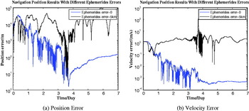
Figure 11. Accuracy comparisons of different ephemeris error.
4.3.4. Navigation Results with Different Integration Step Size
In this simulation, the filter period and measurement of sample interval is assumed to equal the integration step size. The navigation results with integration step size of 6, 60, and 600 s are provided in Figure 12, and the detailed results and the theoretical value of time cost and the simulation value of time cost are given in Table 9. As shown in Figure 12 and Table 9, the estimation error is highly dependent on the selected integration step size. The accuracy increases when the steps are intensive, whereas a small step size requires a larger simulation time which is verified by the inverse proportion relationship between the step size and time cost in theory (Table 9). When the integration step size is selected as 600 s (see red line in Figure 12), the filter is not able to estimate the state properly. Additionally, the navigation error rises suddenly during the encounter.

Figure 12. Accuracy comparisons of different integration step size.
Table 9. Performance comparisons of different integration step size.
The increase of error in Figure 12 is most likely attributable to the giant acceleration error caused by the step. Thus, to promote efficiency, the whole simulation can include different integration step sizes. During the encounter period, the integration step size might be sufficiently small to track the change of acceleration.
4.4. Summary and Case Study
In order to obtain realistic results and provide useful information for space application, a specific Mars-assist explorer case is studied and analysed by summarizing all the results above.
The navigation accuracy and time requirements in that case are shown in Table 10, and the explorer is supposed to have used an ERC32 processor operated at 30 MHz clock rate with a performance of 60MIPS (Wang, Reference Wang2007).
Table 10. Accuracy and time requirements for Mars-assist Mission.

In this case it is assumed that 25% of the processor power is used for orbit determination, 25% is used for attitude determination, the other 50% is used for redundancy. According to the proportionate relationships of the clock rate between the simulation processor and on-board processor, the simulation value of time cost can be transformed to the time cost by the ERC32 processor. Therefore, in that case the simulation time is not a strict restriction.
Assuming that the filter period equals measurement sample interval (60 s), Sun and Mars perturbation in the solar system is suggested for consideration according to the simulation results. In addition, RK4 with 60 s integration step size can be selected to satisfy the mission requirements.
5. CONCLUSIONS
To meet the strict requirements of the navigation system in a GA mission, the factors that mainly influence the dynamic equation are analysed in the current paper by means of comparing the propagation results and the navigation results. Several conclusions can be drawn from the results:
• The propagation results imply that the selection numerical integrator and the standard gravitational parameter uncertainty have a slight influence on the accuracy performance, whereas the integration step size is the dominant impact factor on the real-time performance.
• The navigation results indicate that the filter algorithm is able to decrease the majority of errors. However, the inaccuracy and divergence error caused by ephemeris uncertainty is hardly decreased. Additionally, because of the rapid change of acceleration during the encounter phase, the integration step size is another main factor affecting navigation accuracy, whereas the integration step size is the dominant impact factor on the real-time performance as the propagation results.
• The specific Mars-assist explorer case study using the ERC32 processor shows that the simulation time is not a strict restriction. Therefore, Sun and Mars perturbation in the solar system is suggested for consideration and RK4 with 60 s integration step size can be selected to satisfy the mission requirements.
The conclusions drawn in the present paper help determine the actual capabilities of GA mission navigation system, which is not only beneficial to the GA mission, but to the explorer's encounter with a planet as well.
Future investigation would set up a hardware-in-loop real-time environment to verify the navigation system performance.
ACKNOWLEDGEMENTS
The work described in the current paper was supported by the Research Program for the Supervisor of Excellent PhD Dissertation of Beijing, National Defense Basic Research Program, New Century Program for Excellent Talents of the Ministry of Education of China, and the Astronautics Science and Technology Innovation Fund. The authors would like to thank all members of Science and Technology on Inertial Laboratory and Fundamental Science on Novel Inertial Instrument and Navigation System Technology Laboratory for their useful comments regarding this work.
APPENDIX A NOMENCLATURE
- r=
the heliocentric Cartesian position vector of the explorer.
- v=
the heliocentric Cartesian velocity vector of the explorer.
- (x, y, z)=
the position vector of the celestial body in inertial system.
- (v x,vy,vz)=
the velocity vector of the celestial body in inertial system.
- μ s=
the gravitational constant of the Sun.
- N=
the number of perturbing planets.
- aj=
acceleration caused by non-spherical gravity of assist planet.
- ap=
acceleration caused by thrusters impulse during manoeuvres.
- as=
acceleration caused by radiation pressure.
- a0=
acceleration caused by other factor.
- X=
the state vector.
- g=
dynamic model function.
- w=
process noise.
- Z=
the measurement.
- h=
measurement model function.
- v=
measurement noise.
- (p, l)=
pixel and line of the celestial body centre.
- K=
scales, rotation of the pixel and line axes.
- f=
the sensor focal length.
- (x 2d, y 2d)=
the coordinates of the celestial body centre in the sensor 2-dimensional plane system.
- (p 0, l 0)=
the pixel and line coordinates of the optical axis.
- (x s, y s, z s)=
the position vector of celestial body in sensor system.
- (x i, y i, z i)=
the vector of the celestial body in inertial system.
- Abi=
the transform matrix from the inertial system to the explorer body system, derived via attitude information.
- Asb=
the transform matrix from explorer body system to sensor system.
- n=
the reference time cost.


